


Chapter 8 Quantitative Analysis: Correlation and Regression
Paul Kunesh
School of Business, Liberty University
BUSI820: Quantitative Research Methods (D04)
Dr. David Danley
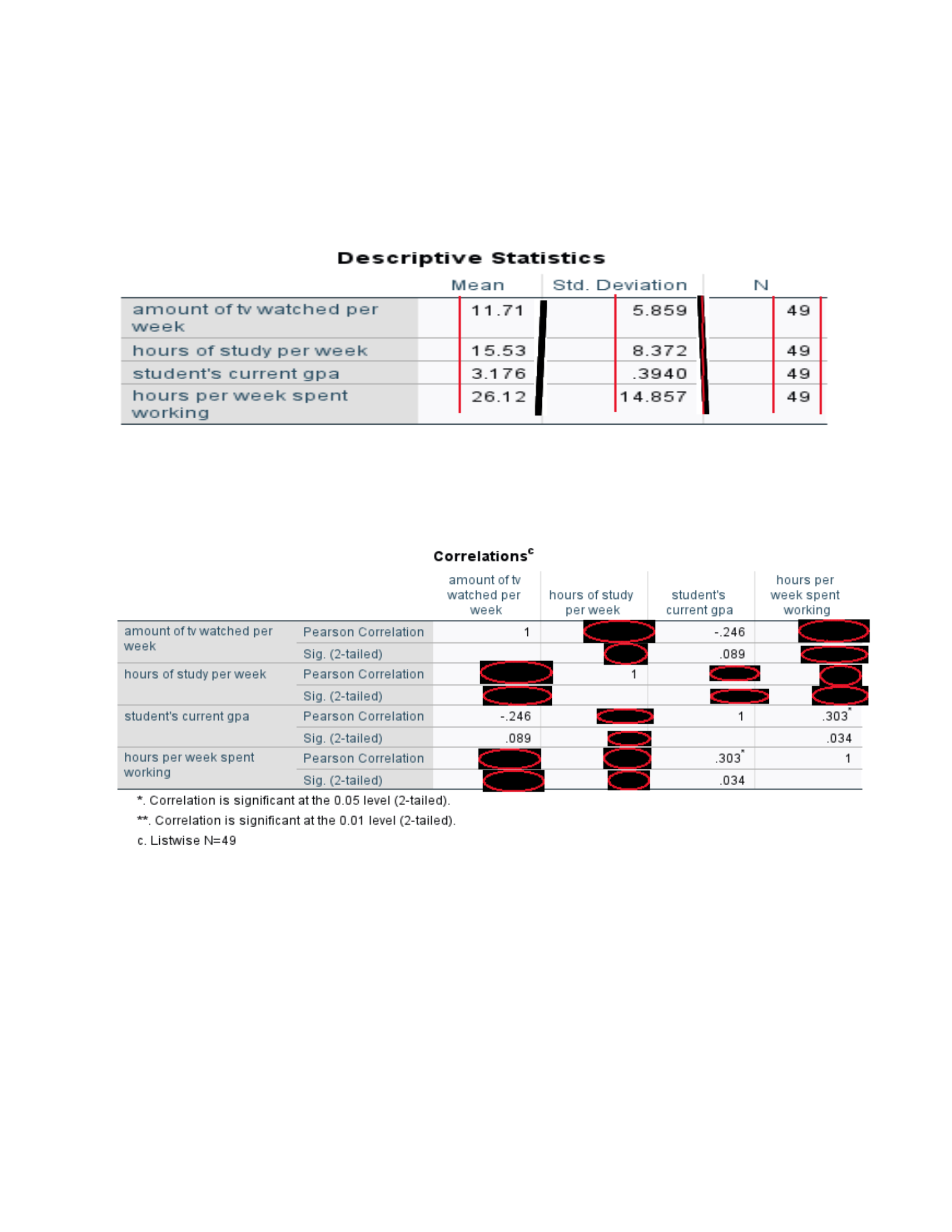
November 30, 2025
Author Note
Paul Kunesh
I have no known conflict of interest to disclose.
Correspondence concerning this article should be addressed to Paul Kunesh.
Email: [email protected]

BUSI820: Quantitative Research Methods (D04)
Table of Contents
8.1 Correlation.................................................................................................................................2
8.2 Correlational Analysis...............................................................................................................4
8.3 Correlation Matrix.....................................................................................................................6
8.4 Gender at Birth and Same Sex Parent’s Height.........................................................................8
References......................................................................................................................................11
1 November 30, 2025

BUSI820: Quantitative Research Methods (D04)
8.1 Correlation
Q. 8.1 What is the correlation between student’s height and parent’s height? Also produce a
scatterplot. Interpret the results, including statistical significance, direction, and effect size.
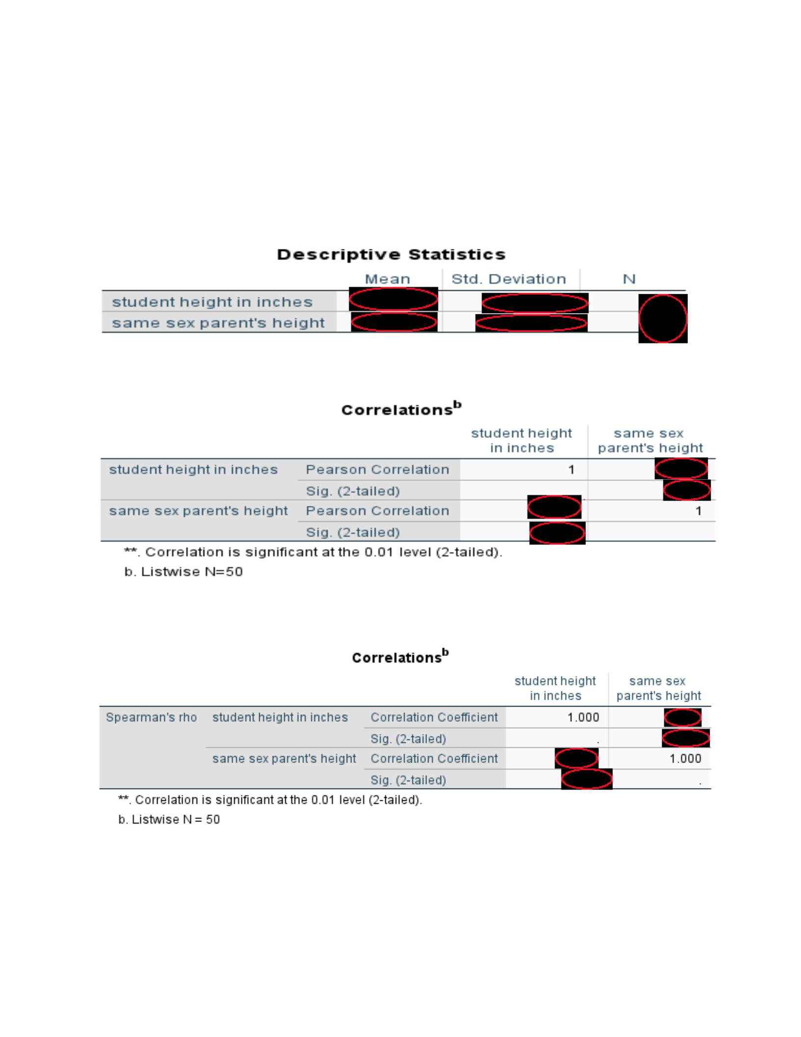
As indicated by Figure 1 the same sex parent’s mean height was 66.78 with a standard
deviation of 5.10. Additionally, the student’s mean height was 67.3 with a standard deviation of
3.94. The Pearson correlation between student height and parent height was r = .842 as listed in
Figure 2. This indicates a strong positive relationship, meaning that higher parent height is
associated with higher student height. Given the sample size N = 50, an r of .842 is statistically
significant at p < .001. This shows that the likelihood of observing such a strong correlation by
chance is extremely low. For effect size, Morgan et al. (2020) classify correlations around .10 as
small, .30 as moderate, and .50 or higher as large. Therefore, r = .842 represents a large effect
size, demonstrating a substantial and meaningful association between the two variables.
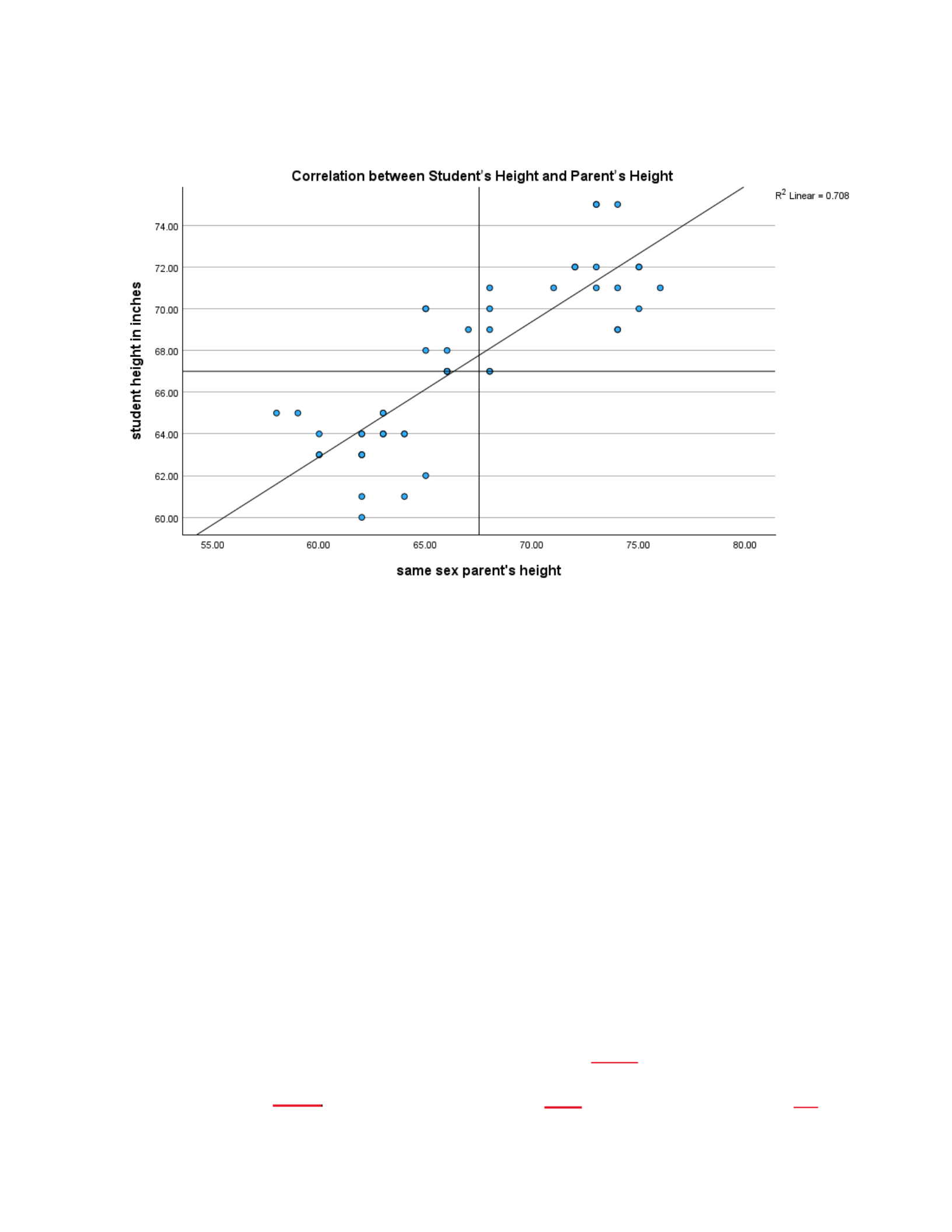
The scatterplot shown in Figure 4 shows a clear upward linear pattern, indicating that as
parent height increases, student height also tends to increase. The points are relatively tight and
closely clustered around an implied straight line, which visually reflects a strong linear
relationship consistent with the calculated correlation of r = .842. There are no major outliers that
break the pattern. While there is some natural variability in the data that parents around 65 inches
are producing children between roughly 62–70 inches, the overall trend remains highly
consistent. The data points spread more vertically in the midrange heights, but the relationship
remains linear and strong across the entire scale. The scatterplot does not show any curvature or
nonlinear pattern. Instead, the pattern is strictly linear, which supports the appropriateness of
Pearson’s r. The distribution also suggests the spread of student height values appears consistent
across different parent height levels which is a condition Morgan et al. (2020) note as important
2 November 30, 2025
BUSI820: Quantitative Research Methods (D04)
when interpreting correlations. The results of the scatterplot provide strong visual evidence that
taller parents generally have taller children, reinforcing the statistical outcome and indicating a
substantial, reliable association.
Figure 1
Figure 2
Figure 3
3 November 30, 2025
BUSI820: Quantitative Research Methods (D04)
Figure 4
8.2 Correlational Analysis
Q. 8.2 Write a question that can be answered via correlational analysis with two approximately
normal or scale variables. Run the appropriate statistics to answer the question. Interpret the
results.
Is there a relationship between the number of hours students work per week and their current
GPA?
Both variables listed above in the question, weekly work hours and GPA, are scale
variables and approximately normal, making them appropriate for correlational analysis. To
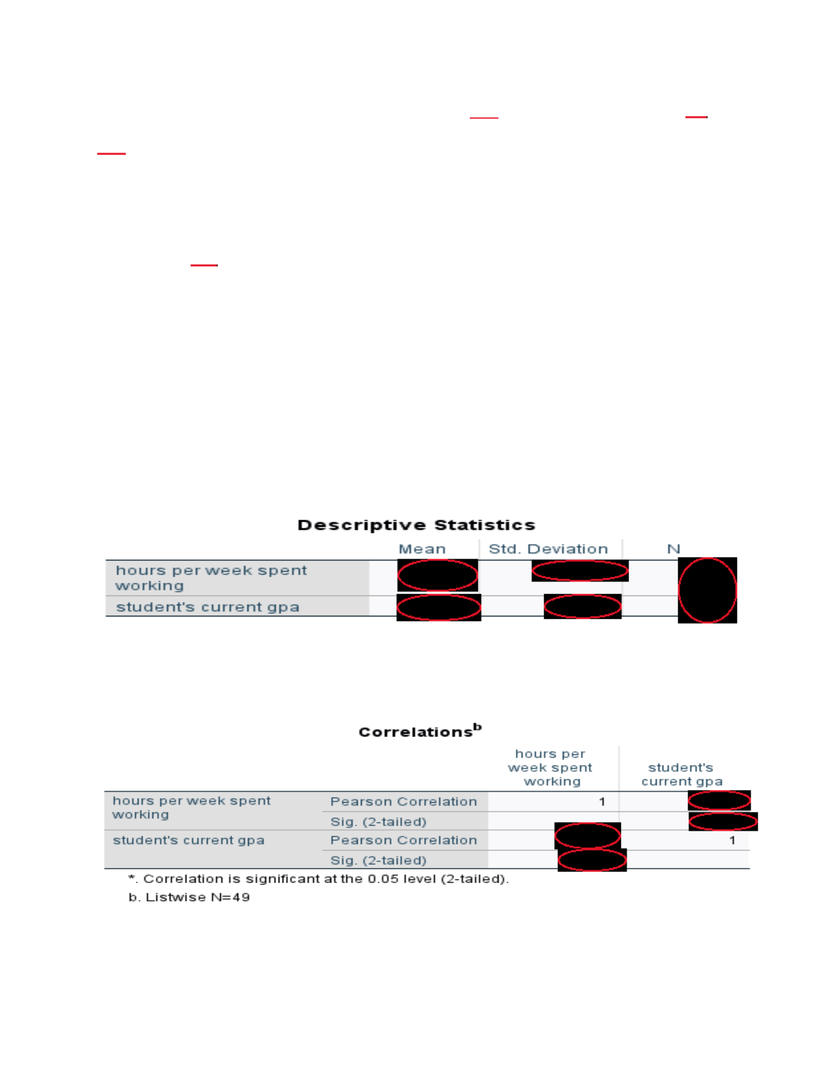
answer the proposed question a Pearson correlation was computed using data from 49 students.
The descriptive statistics show that students work an average of 26.12 hours per week, with a
standard deviation of 14.86, and have an average GPA of 3.18 with a standard deviation of .39.
4 November 30, 2025
BUSI820: Quantitative Research Methods (D04)
The correlation between hours worked and GPA was r = .303, with a significance level of p
= .034. The findings show a statistically significant positive link between the number of hours
students work each week and their GPA. The result is statistically meaningful, suggesting that
there is a genuine relationship between the two variables rather than a random fluctuation. The
correlation of .303 indicates a small-to-moderate effect, meaning that students who work more
hours tend to have slightly higher GPAs. Although the effect is not large, it is still meaningful.
As Morgan et al. (2020) explain, correlations of this size reflect a real but modest association,
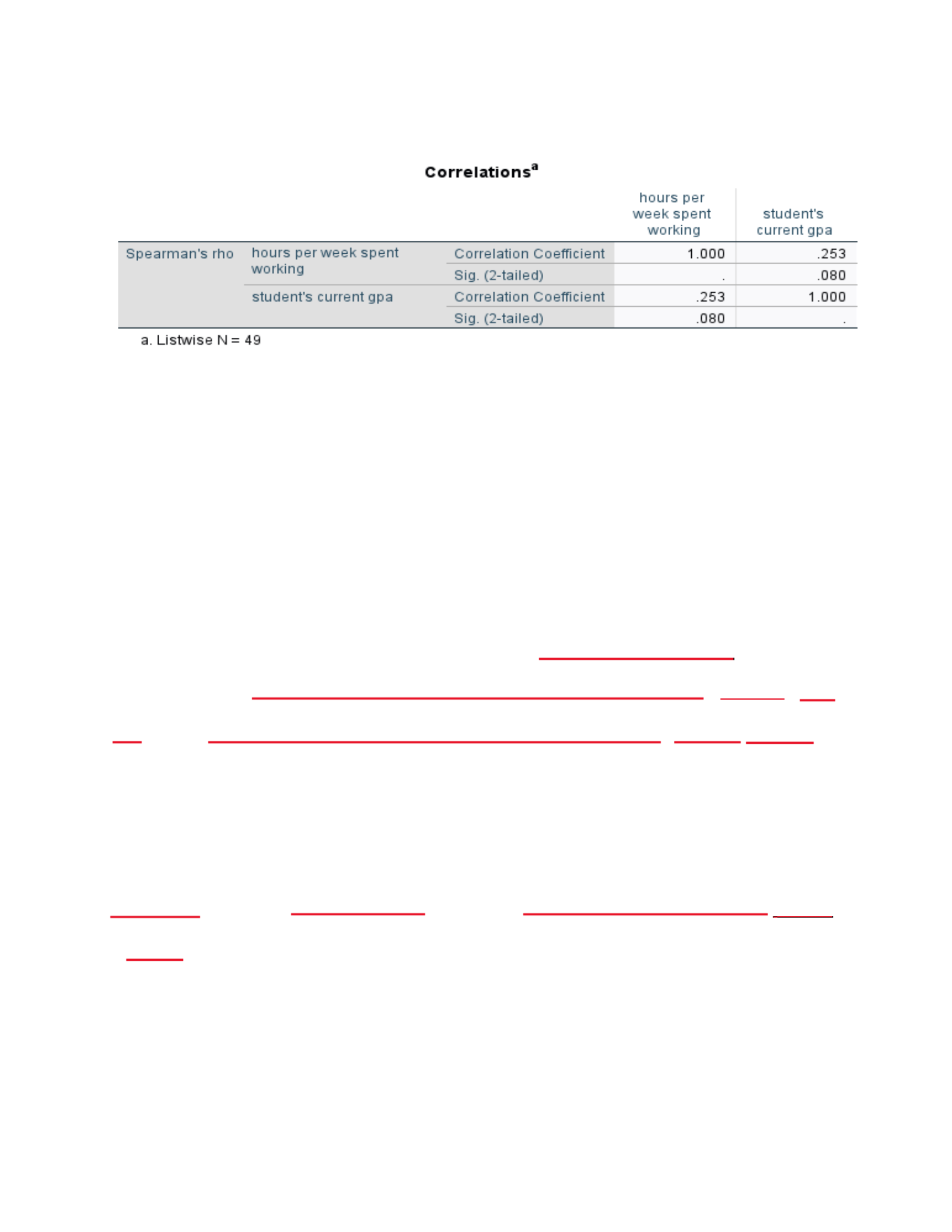
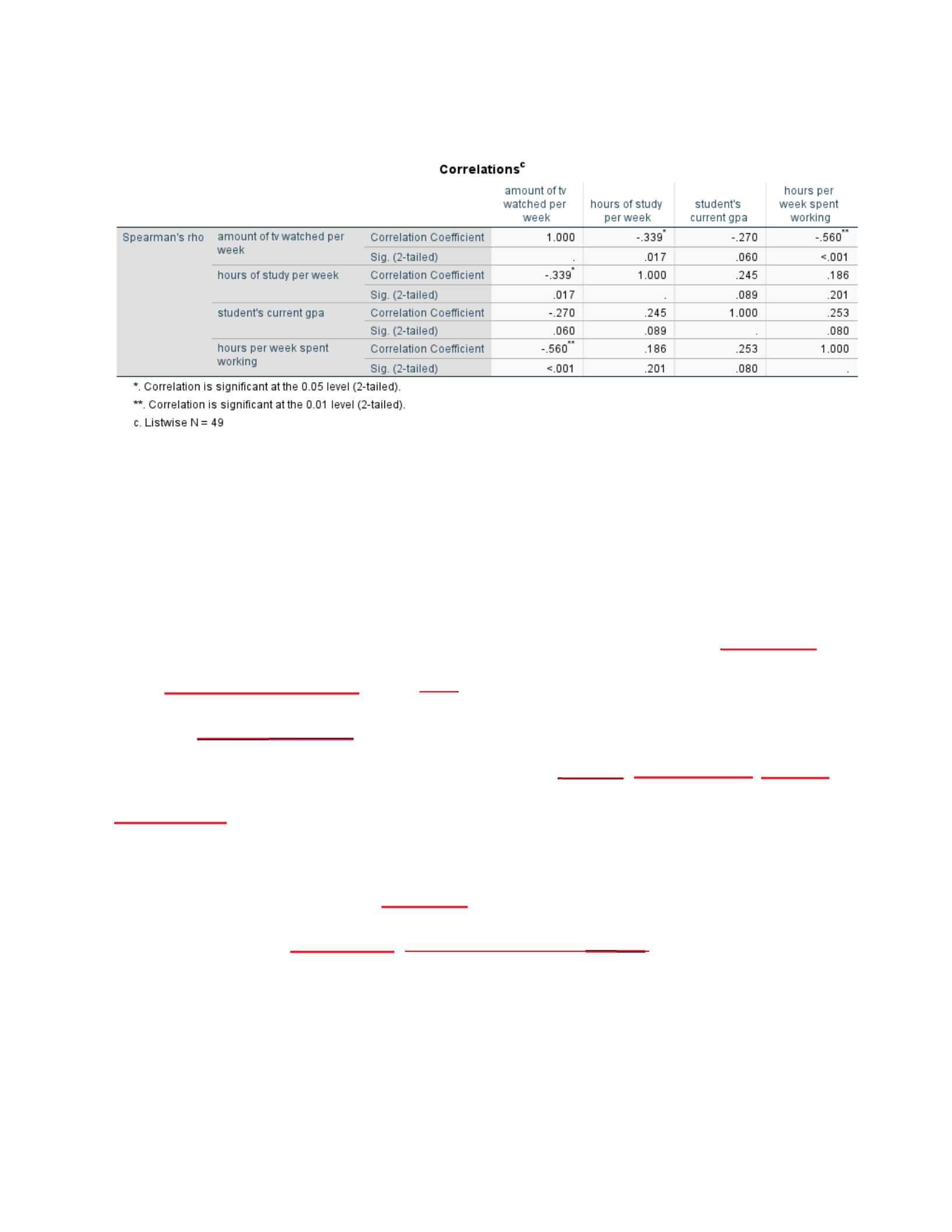
reminding us that many other factors also play a role in shaping GPA. Spearman’s RHO was
included but not needed since this analysis aligns with the assumptions for Pearson’s r, making
Pearson’s the preferred and most informative statistic for these variables.
Figure 5
Figure 6
5 November 30, 2025
BUSI820: Quantitative Research Methods (D04)
Figure 7
8.3 Correlation Matrix
Q. 8.3 Make a correlation matrix using at least four appropriate variables. Identify, using the
variable names, the two strongest and two weakest correlations. What were the r and p values
for each correlation?
I created a Pearson correlation matrix to examine linear associations among four
continuous variables which are amount of TV watched per week, hours of study per week,
students’ current GPA, and hours worked per week. The two strongest correlations between the
variables were the negative relationship between TV watched and hours worked r = –.541, p
< .001 and the negative relationship between TV watched and hours studied r = –.358, p = .011.
These results indicate that students who watch more TV tend to work more hours and study
fewer hours, patterns that Morgan et al. (2020) note are typical of moderate correlations that
represent meaningful, systematic associations. In contrast, the weakest correlations were between
hours studied and GPA r = .114, p = .436 and between hours studied and hours worked r = .219,
p = .131, both of which were small and nonsignificant. As Morgan et al. (2020) explain, such
low r values reflect trivial linear relationships, suggesting that these variables do not
meaningfully predict one another. The matrix clearly shows that only the correlations involving
6 November 30, 2025
BUSI820: Quantitative Research Methods (D04)
TV viewing were strong enough to be considered meaningful, while the others showed minimal
or no linear association.
Figure 8
Figure 9
7 November 30, 2025
BUSI820: Quantitative Research Methods (D04)
Figure 10
8.4 Gender at Birth and Same Sex Parent’s Height
Q. 8.4 Is there a combination of gender at birth and same-sex parent’s height that significantly
predicts student’s height?
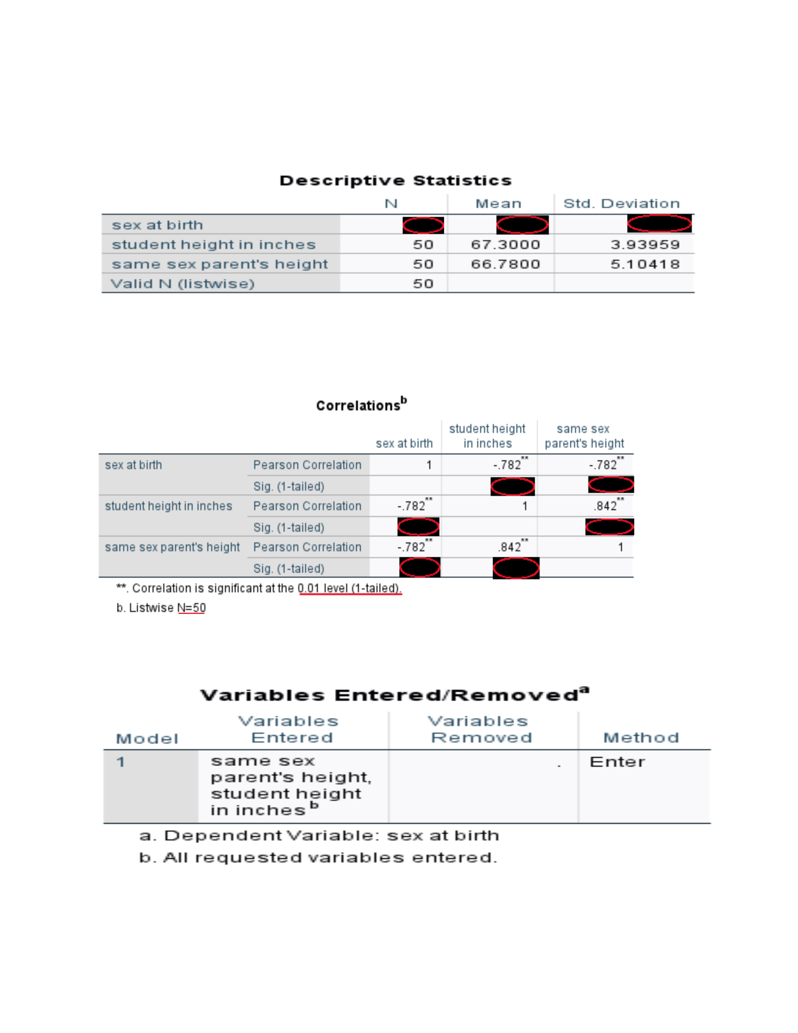
The combination of gender at birth and same-sex parent’s height significantly predicts
student height. Descriptive statistics in Figure 11 indicated that sex at birth had a mean of 1.48
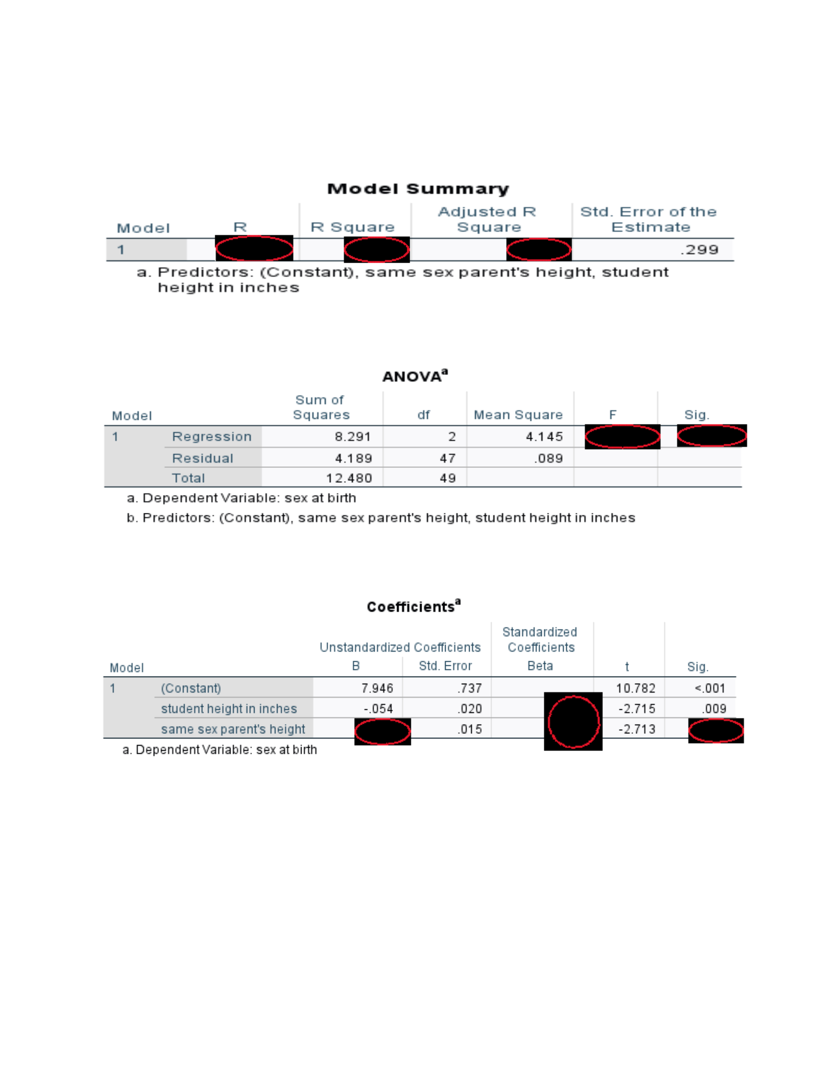
with a standard deviation of .505 and an N=50. The multiple regression model was statistically
significant, F = 46.512, p < .001, demonstrating that these two predictors together explain a large
amount of variance in student height. The model fit indices R = .815, R square = .664, adjusted
Rsquare = .650 show that about 66% of the variability in student height is accounted for by
gender at birth and the height of the same-sex parent, which Morgan et al. (2020) describe as a
strong predictive relationship. Both Betas -.425 and predictors, same-sex parent height B =
–.042, p = .009 and gender at birth p < .001 were individually significant and each contributed
meaningfully to the model. The findings clearly indicate that gender at birth and same-sex parent
height together form a statistically significant and meaningful predictor set for student height,
consistent with the regression interpretation guidelines outlined by Morgan et al. (2020).
8 November 30, 2025
BUSI820: Quantitative Research Methods (D04)
Figure 11
Figure 12
Figure 13
9 November 30, 2025
BUSI820: Quantitative Research Methods (D04)
Figure 14
Figure 15
Figure 16
10 November 30, 2025

BUSI820: Quantitative Research Methods (D04)
References
Morgan, G., Leech, N., Gloeckner, G., Barrett, K. (2020). IBM SPSS for Introductory Statistics
(6th Ed.). New York, NY
11 November 30, 2025

