


Course and Assignment Number
01/02/2021 1
Working with Variables, Z Scores, Population and Interpreting Output-2
Student’s Name
Institution Affiliation
Date

Course and Assignment Number
01/02/2021 2
Table of Contents
A2.1: Chapter 4, Problem 4.1; Descriptive Statistics for the Ordinal and Scale Variables ...3
A2.2: Chapter 4, Problem 4.2, Boxplots for One Variable and for Multiple Variables .........5
A2.3: Chapter 4, Problem 4.3, Boxplots and Stem‐and‐Leaf Plots Split by a Dichotomous
Variable .....................................................................................................................................7
A2.4: Chapter 4, Problem 4.4, Descriptive Statistics for the Dichotomous Variables .......... 10
A2.5: Chapter 4, Problem 4.5, Frequency Tables for a Few Variables ................................. 11
A2.6, Application Problem, Preparing Descriptive Statistics II ............................................ 15
References................................................................................................................................ 20

Course and Assignment Number
01/02/2021 3
A2.1: Chapter 4, Problem 4.1; Descriptive Statistics for the Ordinal and Scale Variables
Output 1: Descriptive Statistics of Ordinal Variables
N
Range
Minim
um
Maxim
um
Mean
Std.
Deviati
on
Varian
ce
Skewness
Kurtosis
Statisti
c
Statisti
c
Statisti
c
Statisti
c
Statisti
c
Statisti
c
Statisti
c
Statisti
c
Std.
Error
Statisti
c
Std.
Error
father's education
73
8
2
10
4.73
2.830E0
8.007E0
.684
.281
-1.047E0
.555
mother's education
75
8
2
10
4.11
2.240E0
5.015E0
1.124E0
.277
.164
.548
grades in h.s.
75
6
2
8
5.68
1.570E0
2.464E0
-.332
.277
-.763
.548
item01 motivation
74
3
1
4
2.96
.928
.861
-.763
.279
-.093
.552
item02 pleasure
75
3
1
4
3.52
.906
.821
-1.910E0
.277
2.571E0
.548
item03 competence
74
3
1
4
2.82
.897
.804
-.579
.279
-.249
.552
item04 low motiv
74
3
1
4
2.16
.922
.850
.422
.279
-.597
.552
item05 low comp
75
3
1
4
1.61
.971
.943
1.581E0
.277
1.390E0
.548
item06 low pleas
75
3
1
4
2.43
.975
.951
-.058
.277
-.997
.548
item07 motivation
75
3
1
4
2.76
1.051E0
1.104E0
-.433
.277
-.975
.548
item08 low motiv
75
3
1
4
1.95
.914
.835
.653
.277
-.422
.548
item09 competence
74
3
1
4
3.32
.760
.578
-1.204E0
.279
1.645E0
.552
item10 low pleas
75
3
1
4
1.41
.737
.543
1.869E0
.277
3.063E0
.548
item11 low comp
75
3
1
4
1.36
.747
.558
2.497E0
.277
6.188E0
.548
item12 motivation
75
3
1
4
3.00
.822
.676
-.600
.277
.020
.548
item13 motivation
75
3
1
4
2.67
.794
.631
-.320
.277
-.194
.548
item14 pleasure
75
3
1
4
2.84
.717
.515
-.429
.277
.350
.548
item04 reversed
74
3
1
4
2.84
.922
.850
-.422
.279
-.597
.552
item05 reversed
75
3
1
4
3.39
.971
.943
-1.581E0
.277
1.390E0
.548
item08 reversed
75
3
1
4
3.05
.914
.835
-.653
.277
-.422
.548
item11 reversed
75
3
1
4
3.64
.747
.558
-2.497E0
.277
6.188E0
.548
Valid N (listwise)
69

Course and Assignment Number
01/02/2021 4
Output 2: Descriptive Statistics on Scale Variables
N
Range
Minimu
m
Maxi
mum
Mean
Std.
Deviatio
n
Varianc
e
Skewness
Kurtosis
Statis
tic
Statist
ic
Statistic
Statisti
c
Statistic
Statistic
Statistic
Statisti
c
Std.
Error
Statistic
Std.
Error
math
achievement
test
75
2.53E
1
-1.67
2.37E
1
1.2564E
1
6.67031
E0
44.493
.044
.277
-.940
.548
mosaic,
pattern test
75
60.0
-4.0
56.0
27.413
9.5738
91.658
.529
.277
3.106
.548
visualization
test
75
1.50E
1
-.25
1.48E
1
5.2433
3.91203
E0
15.304
.536
.277
-.398
.548
visualization 2
75
1.50E
1
.00
1.50E
1
5.1067
3.77518
E0
14.252
.526
.277
-.498
.548
scholastic
aptitude test -
math
75
480
250
730
490.53
94.553
8.940E3
.128
.277
.943
.548
mosaic pattern
test 2
75
5.60E
1
.00
5.60E
1
2.7480E
1
9.34816
E0
87.388
.882
.277
3.063
.548
competence
scale
73
3.00
1.00
4.00
3.2945
.66450
.442
-
1.634E
0
.281
3.037
.555
motivation
scale
73
2.83
1.17
4.00
2.8744
.63815
.407
-.570
.281
-.034
.555
Valid N
(listwise)
71
The descriptive statistics analysis on the ordinal aand scale variables have been done on
the datset to showcase the general insights of the underlying data. This is done on the SPSS
software using the analyze button and secective descriptive statistics, and finally the descriptives.
The deascriptive measures of central tendency and measure of dispersion and variation are used to
further elucidate the nature and distribution of variables. The measure of central tendency is the
Course and Assignment Number
01/02/2021 5
mean, the measures of dispersion include the range and the variance, and the measure of
distribution includes the skewness and kurtosis. The results from the practical analysis using the
steps given are shown on Output 1 and Output attached above. The analysis above indicates that
there are variables with missing information. The variables with complete infromeation are
respresented by N=75, while the lesser values of N indicate the existence of missintg values in the
data. For instance, item01 motivation on Output 1, and Motivation 1 on Output 2 are some of the
variables with missing information. The skewness and kurtosis measures indicates the distribution
of the varaibles where the some variables falls between -1 and +1, while others do not fall in this
threshold.
A2.2: Chapter 4, Problem 4.2, Boxplots for One Variable and for Multiple Variables
The box plot of an individual variable is done using the graphs option on SPSS, then we
select the legacy dialogue, and then selecting the boxplot. To produce the box-plot, the simple
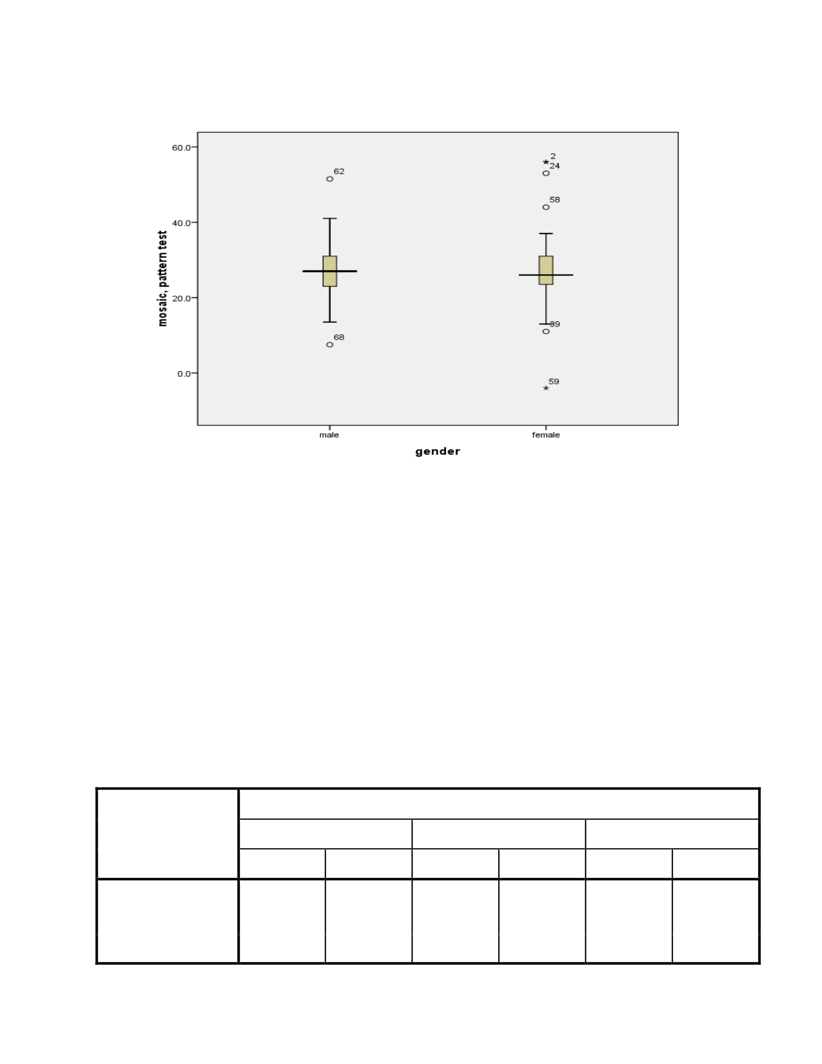
cases option is selected. The first boxplot is on the mosaic tests results compared to the gender of
the participants. The boxplot is attached below;
Case Processing Summary
gender
Cases
Valid
Missing
Total
N
Percent
N
Percent
N
Percent
mosaic, pattern test
male
34
100.0%
0
.0%
34
100.0%
female
41
100.0%
0
.0%
41
100.0%
Course and Assignment Number
01/02/2021 6
Figure 1: Boxplot on Mosaic and Pattern Test Vs Gender
The results indicate the male gender has a mean score in mosaic and pattern test have higher scores
compared to that of the females with a mean of 68 and 39, respectively. The case processing
summary indicates that the male and female students are 34 and 41, respectively (Morgan et al.,
2013). . The value for N in this case is 75 which implies that there are no missing values present.
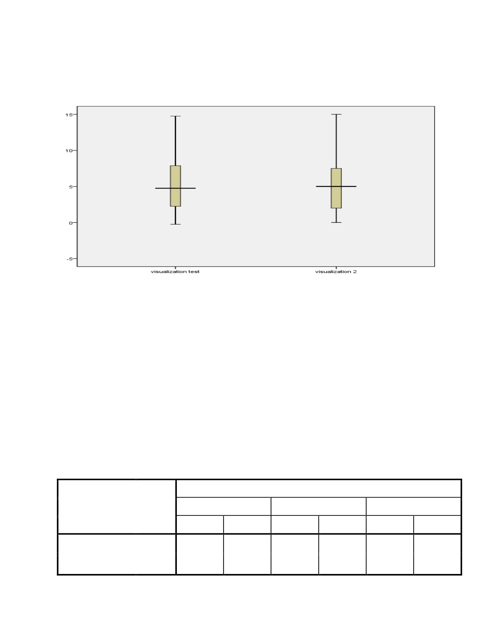
The following are the box-plot of two different variables in the same plot, for visualization test 1
and 2;
Case Processing Summary for Visualization Test 1 and 2
Cases
Valid
Missing
Total
N
Percent
N
Percent
N
Percent
visualization test
75
100.0%
0
.0%
75
100.0%
visualization 2
75
100.0%
0
.0%
75
100.0%
Course and Assignment Number
01/02/2021 7
Figure 2: Box Plots on Visualization 1 and 2 Tests
The case processing summary indicates no missing values while the boxplots indicates an even
distribution of visualization test 1 and 2 since no outliers are observed.
A2.3: Chapter 4, Problem 4.3, Boxplots and Stem‐and‐Leaf Plots Split by a Dichotomous
Variable
An example of a dichotomous variable is the gender of the students whereby the students’
performance is compared to their respective gender orientation. The variable has only two specific
options of choice which makes them a dichotomous variable (Morgan et al., 2013) . The box plots
will indicate the distribution of the students who took algebra1 course.
Case Processing Summary
gender
Cases
Valid
Missing
Total
N
Percent
N
Percent
N
Percent
visualization test
male
34
100.0%
0
.0%
34
100.0%
female
41
100.0%
0
.0%
41
100.0%

Course and Assignment Number
01/02/2021 8
Descriptives of Visualization Tests 1 Vs Gender
Gender
Statistic
Std. Error
visualization
test
male
Mean
6.4265
.76671
95% Confidence
Interval for Mean
Lower Bound
4.8666
Upper Bound
7.9864
5% Trimmed Mean
6.3350
Median
6.0000
Variance
19.987
Std. Deviation
4.47067
Minimum
-.25
Maximum
14.75
Range
15.00
Interquartile Range
7.31
Skewness
.232
.403
Kurtosis
-.924
.788
female
Mean
4.2622
.48506
95% Confidence
Interval for Mean
Lower Bound
3.2818
Upper Bound
5.2425
5% Trimmed Mean
4.1741
Median
4.7500
Variance
9.647
Std. Deviation
3.10592
Minimum
-.25
Maximum
11.00
Range
11.25
Interquartile Range
5.00
Skewness
.388
.369
Kurtosis
-.629
.724

Course and Assignment Number
01/02/2021 9
Stem and Leaf Plots;
visualization test Stem-and-Leaf Plot for
gender= male
Frequency Stem & Leaf
3.00 -0. 000
12.00 0. 111222333444
12.00 0. 666677889999
7.00 1. 1113344
Stem width: 10.0
Each leaf: 1 case(s)
visualization test Stem-and-Leaf Plot for
gender= female
Frequency Stem & Leaf
4.00 -0. 2222
.00 0.
7.00 1. 0000000
3.00 2. 222
6.00 3. 555557
7.00 4. 7777777
2.00 5. 00
3.00 6. 000
3.00 7. 222
2.00 8. 77
3.00 9. 777
.00 10.
1.00 11. 0
Stem width: 1.00
Each leaf: 1 case(s)
Course and Assignment Number
01/02/2021 10
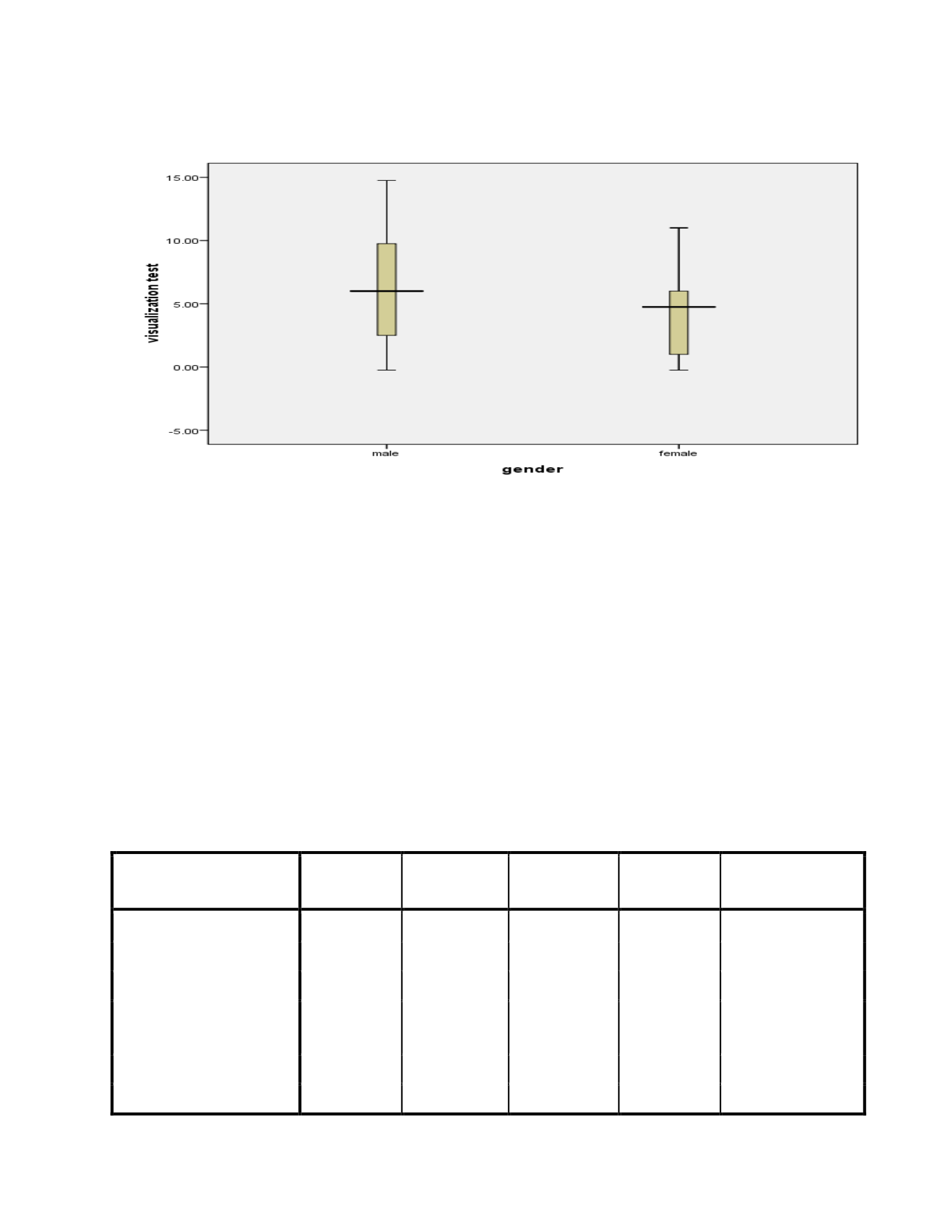
Figure 3: Box plot on Visualization test 1 Performance VS Gender
The analysis indicates the higher performance of the male students compared to the female students
with a mean score of 6.42 and 4.21, respectively. There are no missing variables for these variables
and outliers as indicated on Figure 3.
A2.4: Chapter 4, Problem 4.4, Descriptive Statistics for the Dichotomous Variables
The descriptive statistics will be done by selecting a variable such as algebra 1 and 2 where the
students indicate whether they have done the course or not. The following is the descriptive
statistics of dichotomous variables;
Descriptive Statistics of Dichotomous Variables
N
Minimum
Maximum
Mean
Std. Deviation
algebra 1 in h.s.
75
0
1
.79
.412
algebra 2 in h.s.
75
0
1
.47
.502
geometry in h.s.
75
0
1
.48
.503
trigonometry in h.s.
75
0
1
.27
.445
calculus in h.s.
75
0
1
.11
.311
Valid N (listwise)
75

Course and Assignment Number
01/02/2021 11
The above results indicate that there are no missing values on the dichotomous variables selected
for the descriptive statistics analysis because N, valid listwise is 75 for all the variables. The mean
of geometry is 0.48 which implies that the students taking geometry are 48% of the total number
of the students (Morgan et al., 2013). Similarly, the students not taking geometry is approximately
52%. The students taking calculus are represented by 11% of the total students while the ones not
taking calculus are represented by approximately 89 (Morgan et al., 2013).
A2.5: Chapter 4, Problem 4.5, Frequency Tables for a Few Variables
The frequency tables are in the analysis tab on SPSS and we select the descriptive statistics
option. Both dichotomous variables and ordinal variables can be used in the frequency table
analysis so as to specify the specification of the distribution of individual variables (Morgan et al.,
2013). The following are the descriptive statistics of individual variables;
Descriptive Statistics of Variables
gender
mother's
education
father's
education
ethnicity
religion
math grades
N
Valid
75
75
73
73
67
75
Missing
0
0
2
2
8
0
Mean
.55
4.11
4.73
1.77
1.76
.41
Median
1.00
3.00
3.00
1.00
2.00
.00
Std. Deviation
.501
2.240
2.830
1.021
.780
.496
Variance
.251
5.015
8.007
1.042
.609
.246
Skewness
-.191
1.124
.684
1.052
.450
.359
Std. Error of Skewness
.277
.277
.281
.281
.293
.277
Kurtosis
-2.018
.164
-1.047
-.192
-1.211
-1.923
Std. Error of Kurtosis
.548
.548
.555
.555
.578
.548
Range
1
8
8
3
2
1
Minimum
0
2
2
1
1
0
Maximum
1
10
10
4
3
1
The following are frequency tables for the selected variables;
Course and Assignment Number
01/02/2021 12
Frequency Table on Gender of the Students
Frequency
Percent
Valid Percent
Cumulative
Percent
Valid
male
34
45.3
45.3
45.3
female
41
54.7
54.7
100.0
Total
75
100.0
100.0
Majority of the students are females which are represented by N=41, 54.7% while the male
students are 45.3% of the total students.
Frequency Distribution of Mother's Education
Frequency
Percent
Valid Percent
Cumulative
Percent
Valid
< h.s.
17
22.7
22.7
22.7
h.s. grad
31
41.3
41.3
64.0
< 2 yrs voc
2
2.7
2.7
66.7
2 yrs voc
5
6.7
6.7
73.3
< 2 yrs coll
7
9.3
9.3
82.7
> 2 yrs coll
5
6.7
6.7
89.3
coll grad
3
4.0
4.0
93.3
master's
3
4.0
4.0
97.3
MD/PhD
2
2.7
2.7
100.0
Total
75
100.0
100.0
Course and Assignment Number
01/02/2021 13
Majority of the mothers, represented by N=31, 41.3% are high school graduates while the minority
of the mothers are MD/PHD graduates and <2years vocation represented by N=2, 2.7%.
Frequency Distribution on Father's Education
Frequency
Percent
Valid
Percent
Cumulative
Percent
Valid
< h.s. grad
22
29.3
30.1
30.1
h.s. grad
16
21.3
21.9
52.1
< 2 yrs voc
3
4.0
4.1
56.2
2 yrs voc
8
10.7
11.0
67.1
< 2 yrs coll
4
5.3
5.5
72.6
> 2 yrs coll
1
1.3
1.4
74.0
coll grad
7
9.3
9.6
83.6
master's
6
8.0
8.2
91.8
MD/PhD
6
8.0
8.2
100.0
Total
73
97.3
100.0
Missing
System
2
2.7
Total
75
100.0
Majority of the fathers, represented by N=22, 29.3% are <high school graduates while the minority
of the fathers are >2years college represented by N=1, 1.3%.
Frequency Distribution of Math grades
Frequency
Percent
Valid
Percent
Cumulative
Percent
Valid
less A-B
44
58.7
58.7
58.7
most A-B
31
41.3
41.3
100.0
Total
75
100.0
100.0
Course and Assignment Number
01/02/2021 14
Most of the students, represented by N=44, 58.7% scored less than A-B, while the rest, represented
by N=31, 41.3% scored in the category A-B.
Frequency Distribution of Ethnicity
Frequency
Percent
Valid
Percent
Cumulative
Percent
Valid
Euro-Amer
41
54.7
56.2
56.2
African-
Amer
15
20.0
20.5
76.7
Latino-Amer
10
13.3
13.7
90.4
Asian-Amer
7
9.3
9.6
100.0
Total
73
97.3
100.0
Missing
multiethnic
1
1.3
blank
1
1.3
Total
2
2.7
Total
75
100.0
Frequency Distribution of the Religion
Frequency
Percent
Valid
Percent
Cumulative
Percent
Valid
protestant
30
40.0
44.8
44.8
catholic
23
30.7
34.3
79.1
no religion
14
18.7
20.9
100.0
Total
67
89.3
100.0
Missing
other religion
4
5.3
blank
4
5.3
Total
8
10.7
Total
75
100.0
Course and Assignment Number
01/02/2021 15
A2.6, Application Problem, Preparing Descriptive Statistics II
Using the “college student data.sav” file, do the following problems. Write a short narrative of
your process and an interpretation of your findings. Cut and paste your outputs directly into your
document and refer to them in your interpretation.
a. For the variables with five or more ordered levels, compute the skewness and describe
the results.
The variables with five or more ordered variables in this dataset includes (positive
evaluation, institution), (positive evaluation, major), (positive evaluation, facilities),
(positive evaluation, social life). The descriptive statistics of these variables indicating the
distribution of them based on skewness and Kurtosis is shown below;
Descriptive Statistics of 5-level Variables
N
Skewness
Kurtosis
Statistic
Statistic
Std. Error
Statistic
Std. Error
positive evaluation,
institution
50
.059
.337
-.868
.662
positive evaluation, major
49
-.115
.340
-.524
.668
positive evaluation,
facilities
50
-.136
.337
-.432
.662
positive eval, social life
50
.031
.337
-.880
.662
Valid N (listwise)
49
The Skewness measures for the selected ordinal variables are both negative and positive implying
that they fall between the -1 to+1 threshold (Morgan et al., 2013). The positive evaluation, major
and facilities have a skewness measure of -0.115 and -0.136, respectively. The negative skewness
statistics implies that the distribution of these ordinal variables is approximately normal (Morgan
et al., 2013). The variables with positive measure corresponding to social life and institutional
evaluation are not approximately normally distributed.

Course and Assignment Number
01/02/2021 16
b. Which variables in the data set are approximately normally distributed/scale?
The variables that are normally distributed are positive evaluation, major and facilities
with a skewness statistic estimate of -0.115 and -0.136, respectively.
c. Which ones are ordered but not normal?
The variables that are normally distributed are positive evaluation, social life and
institutional with a skewness statistic estimate of 0.059 and 0.031, respectively.
d. Prepare a stem‐and‐leaf plot for the same sex parent’s height split by gender and discuss
the plots.
Stem and Leaf Plots for Same Sex Parents and Gender of the Students;
same sex parent's height Stem-and-Leaf Plot for
gender= males
Frequency Stem & Leaf
.00 6.
4.00 6. 4455
2.00 6. 67
5.00 6. 88888
1.00 7. 1
6.00 7. 223333
7.00 7. 4444555
1.00 7. 6
Stem width: 10.00
Each leaf: 1 case(s)
same sex parent's height Stem-and-Leaf Plot for
gender= females
Frequency Stem & Leaf
Course and Assignment Number
01/02/2021 17
1.00 Extremes (=<58.0)
1.00 59. 0
3.00 60. 000
.00 61.
7.00 62. 0000000
5.00 63. 00000
1.00 64. 0
2.00 65. 00
4.00 66. 0000
Stem width: 1.00
Each leaf: 1 case(s)
e. Which of the variables are nominal? Run the frequencies for the nominal variables and
other variables with fewer than five levels and discuss the results.
Some of the nominal variables includes the student’s GPA, hours of study per week,
students’ height in inches, amount of tv watched per week, and same sex parents’ height.
gender of student
Frequency
Percent
Valid
Percent
Cumulative
Percent
Valid
males
26
52.0
52.0
52.0
females
24
48.0
48.0
100.0
Total
50
100.0
100.0

Course and Assignment Number
01/02/2021 18
student height in inches
Frequency
Percent
Valid
Percent
Cumulative
Percent
Valid
60
1
2.0
2.0
2.0
61
2
4.0
4.0
6.0
62
1
2.0
2.0
8.0
63
5
10.0
10.0
18.0
64
8
16.0
16.0
34.0
65
4
8.0
8.0
42.0
67
6
12.0
12.0
54.0
68
2
4.0
4.0
58.0
69
4
8.0
8.0
66.0
70
4
8.0
8.0
74.0
71
5
10.0
10.0
84.0
72
5
10.0
10.0
94.0
75
3
6.0
6.0
100.0
Total
50
100.0
100.0
The frequency distribution tables are more appropriate for grouped data, or data in form of
categories based on the results above. The gender orientation of the students is effectively
elucidated using the frequency tables whereby the majority of the college students are male, N=26,
52%, while females are represented by N=24, 48% (Morgan et al., 2013).

Course and Assignment Number
01/02/2021 19
f. Prepare boxplots for student height and for hours of study. Discuss a comparison of the
two plots.

Course and Assignment Number
01/02/2021 20
References
Morgan, G., Leech, N., Gloeckner, G., Barrett, K. (2013). IBM SPSS for Introductory Statistics
(5th Ed.). New York, NY.
Keller, T. (2012), Every Good Endeavor, Riverhead Books, Penguin Group, New York, NY.
Lee, D. K. (2016). Alternatives to P value: confidence interval and effect size. Korean journal of
anesthesiology, 69(6), 555.

