



Mat 275 MATLAB LAB #5
Name: Brandon Grebe
Lab Day and Time: Wednesday
10:30
Instructor: Chowell Puente
Exercise #1
Part A
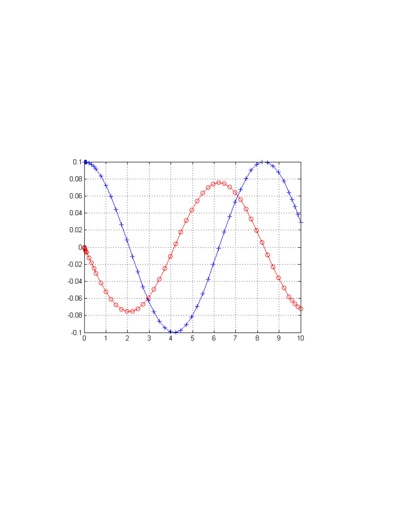
The blue graph is the correct curve for y = y(t). We know this by
looking at the initial conditions. In the problem we were given y(0) = 0.1
and y’(0) = 0. Seeing how the blue curve starts at 0.1 we can assume that
this is the correct graph for the function.
Part B
By looking at the peaks of the blue curve we can guess that the period
will be roughly around three. This was estimated by taking one of the peaks
around 3.1 and comparing it with the next peak which occurred around 6.2.
Given that these are sinusoidal waves we can guess that this difference of
3.1 is actually pi. We can prove this analytically by finding the period of
𝜔0.
𝜔0 = √𝑚/𝑘 = √4/1 = 2
T = 2𝜋
2= 𝝅
Part C
No, this problem is an undamped situation meaning that there is no
friction, wind resistance, or anything affecting the oscillation of this
weight. It will oscillate forever.
Part D
Knowing that the blue curve is our displacement curve we can simply
look at the initial condition as well as all of the peaks of the two curves
and see that the difference between them is 0.1.
Part E
Looking at the graph we can see that the maximum velocity occurs when
the red graph is at its peak. Coincidently when the red cure is at its peak
the displacement curve is at 0. Simple looking at when the blue curve is at
“equilibrium” or 0 will provide us with the time at which the velocity is
greatest.
Estimating these points gives us.
0.77
2.3
3.94
5.48
7.06
8.7
Part F
Returning to our period formula.
T = 2 𝜋
𝜔0 = 2𝜋√𝑚/𝑘
If m(mass) is increased, m/k will be larger than before. This mean the weight
will oscillate for much longer, the period will be greater.
function LAB05ex1
m = 8; % mass [kg]
k = 4; % spring constant [N/m]
omega0 = sqrt(k/m);
y0 = 0.1; v0 = 0; % initial conditions
[t,Y] = ode45(@f,[0,10],[y0,v0],[],omega0); % solve for 0<t<10
y = Y(:,1); v = Y(:,2); % retrieve y, v from Y
figure(1); plot(t,y,'b+-',t,v,'ro-'); % time series for y and v
grid on;
%-----------------------------------------
function dYdt = f(t,Y,omega0)
y = Y(1); v = Y(2);
dYdt = [ v ; -omega0^2*y ];
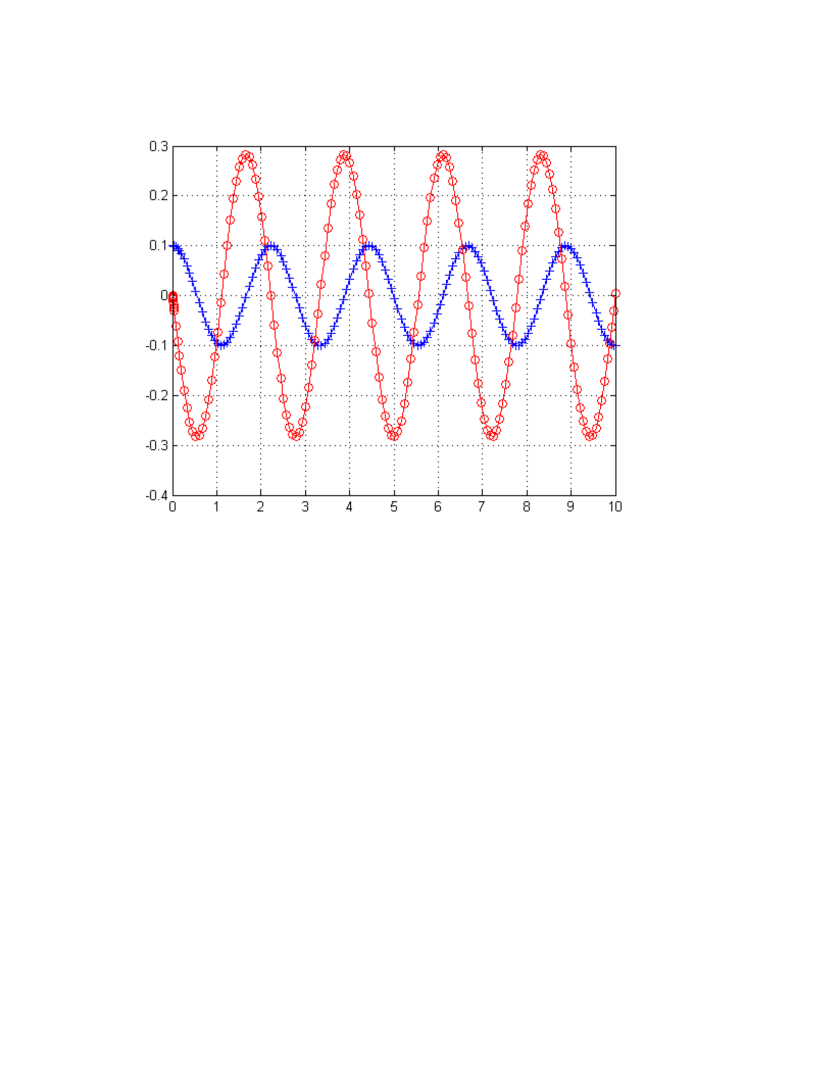
If k is increased, m/k will be smaller than before. This means the stiffness
of the constant is much greater and the period of the oscillating weight will
be much shorter.
function LAB05ex1
m = 4; % mass [kg]
k = 10; % spring constant [N/m]
omega0 = sqrt(k/m);
y0 = 0.1; v0 = 0; % initial conditions
[t,Y] = ode45(@f,[0,10],[y0,v0],[],omega0); % solve for 0<t<10
y = Y(:,1); v = Y(:,2); % retrieve y, v from Y
figure(1); plot(t,y,'b+-',t,v,'ro-'); % time series for y and v
grid on;
%-----------------------------------------
function dYdt = f(t,Y,omega0)
y = Y(1); v = Y(2);
dYdt = [ v ; -omega0^2*y ];
Exercise #2
Part A
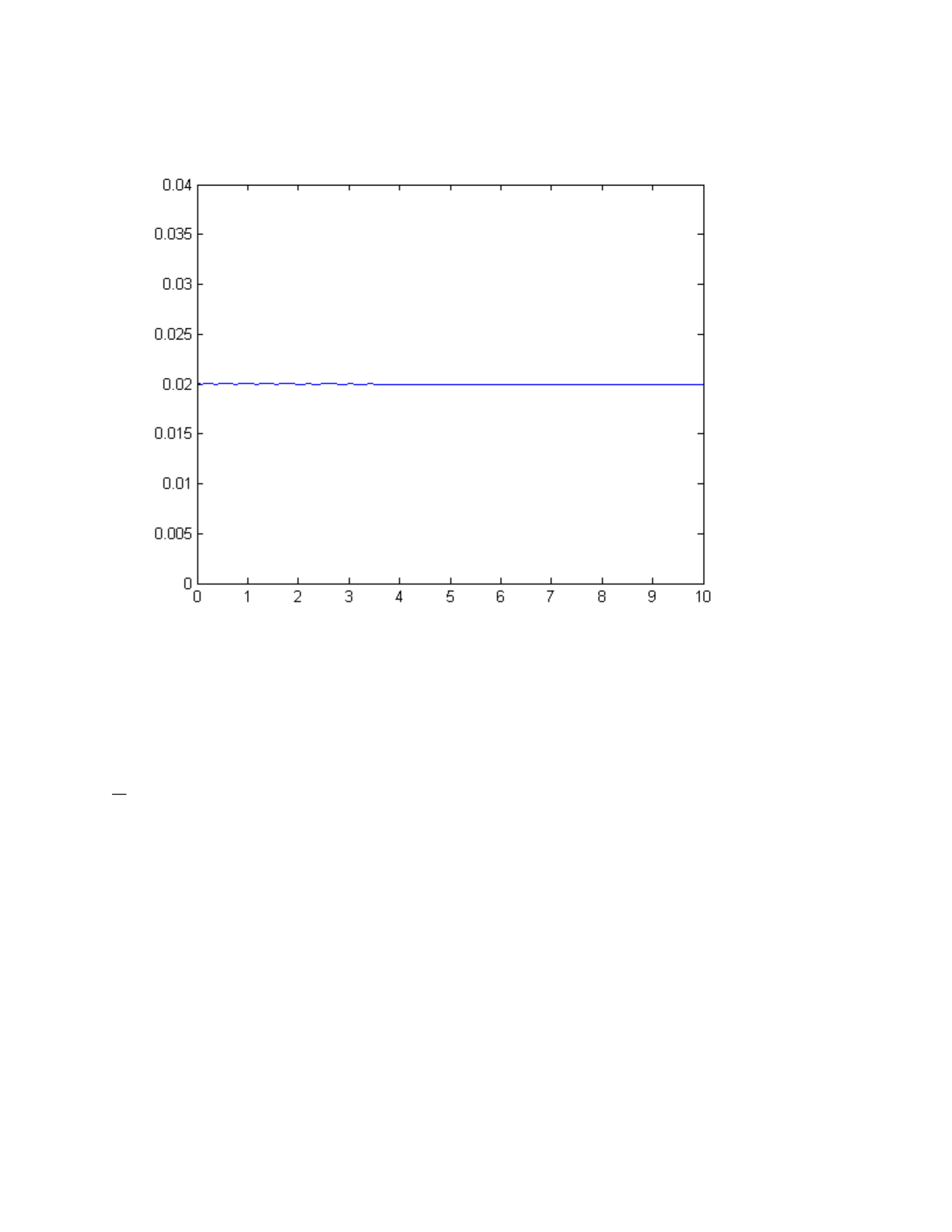
Using the limit feature on MatLab we are able to plot this quantity and
analyze the energy to see if it is conserved or not.
Looking at this graph we see that energy is indeed conserved as it starts
nearly equal to 0.02. The small oscillations seen in the beginning of the
graph are due to random errors.
Part B
From the Differential Equation we have the following equation.
v’ = y’’ = -𝜔02𝑦 = -(k/m)y
We then have:
𝑑𝐸
𝑑𝑡 = 1/2 m2vv’ + 1/2 k2yy’
= mvv’ + kyy’
= my’(-k/m)y + kyy’ = 0
Part C
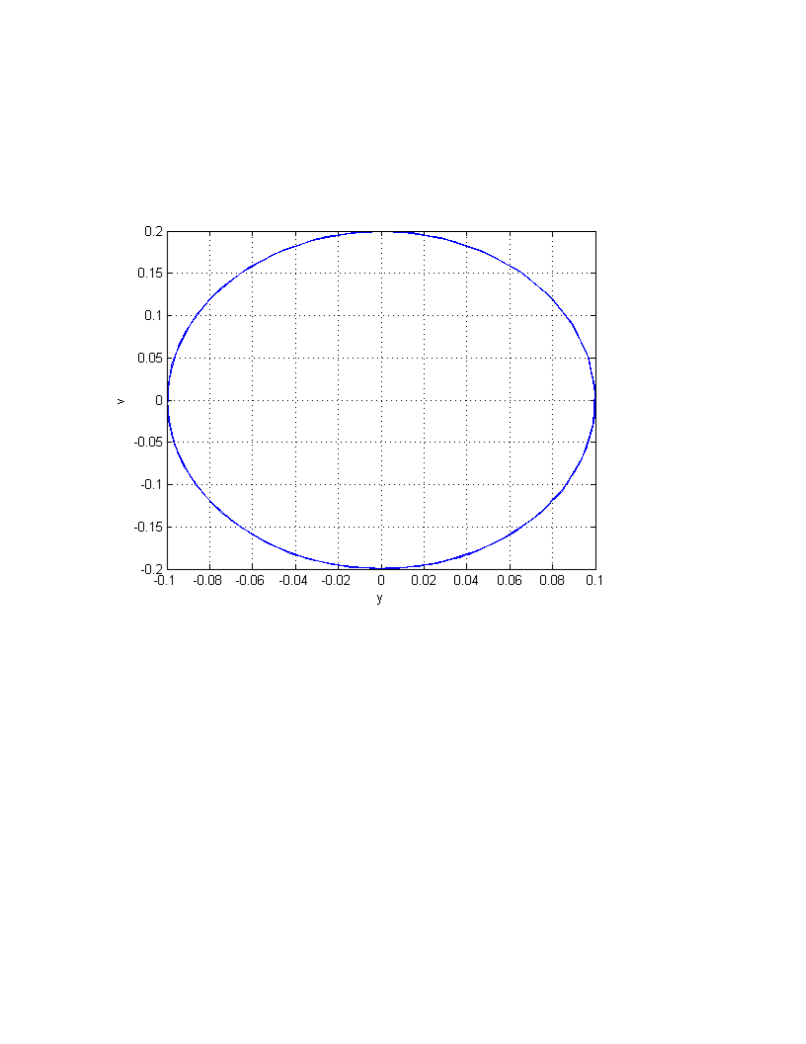
Graphing the phase plot we see that it is an ellipse.
function LAB05ex1
m = 1; % mass [kg]
k = 4; % spring constant [N/m]
omega0 = sqrt(k/m);
y0 = 0.1; v0 = 0; % initial conditions
[t,Y] = ode45(@f,[0,10],[y0,v0],[],omega0); % solve for 0<t<10
y = Y(:,1); v = Y(:,2); % retrieve y, v from Y
figure(1); plot(t,y,'b+-',t,v,'ro-'); % time series for y and v
grid on;
E=m*v.^2/2+k*y.^2/2
figure(2); plot(t,E)
ylim([0,0.04])
figure(3)
plot(y,v);
xlabel('y'); ylabel ('v'); grid on
%-----------------------------------------
function dYdt = f(t,Y,omega0)
y = Y(1); v = Y(2);
dYdt = [ v ; -omega0^2*y ];
This graph is a closed curve. The maximum value of y is 0.1 and the minimum
is -0.1. The maximum value of the velocity is 0.2 and the minimum is -0.2.
The curve never gets close to the origin because this means that y and v
would both have to be zero and the spring would have to come to a complete
stop, which we know is impossible because there is no friction and no loss of
energy.
Exercise #3
Part A
Filling in the function.
function LAB05ex1a
m = 1; % mass [kg]
k = 4; % spring constant [N/m]
c = 1; % friction coefficient [Ns/m]
omega0 = sqrt(k/m); p = c/(2*m);
y0 = 0.1; v0 = 0; % initial conditions
[t,Y] = ode45(@f,[0,10],[y0,v0],[],omega0,p); % solve for 0<t<10
y = Y(:,1); v = Y(:,2); % retrieve y, v from Y
figure(1); plot(t,y,'b+-',t,v,'ro-'); % time series for y and v
grid on;
%-------------------------------------------
function dYdt = f(t,Y,omega0,p)
y = Y(1); v = Y(2);
dYdt = [ v ; -omega0^2*y-2*p*v ]; % fill-in dv/dt
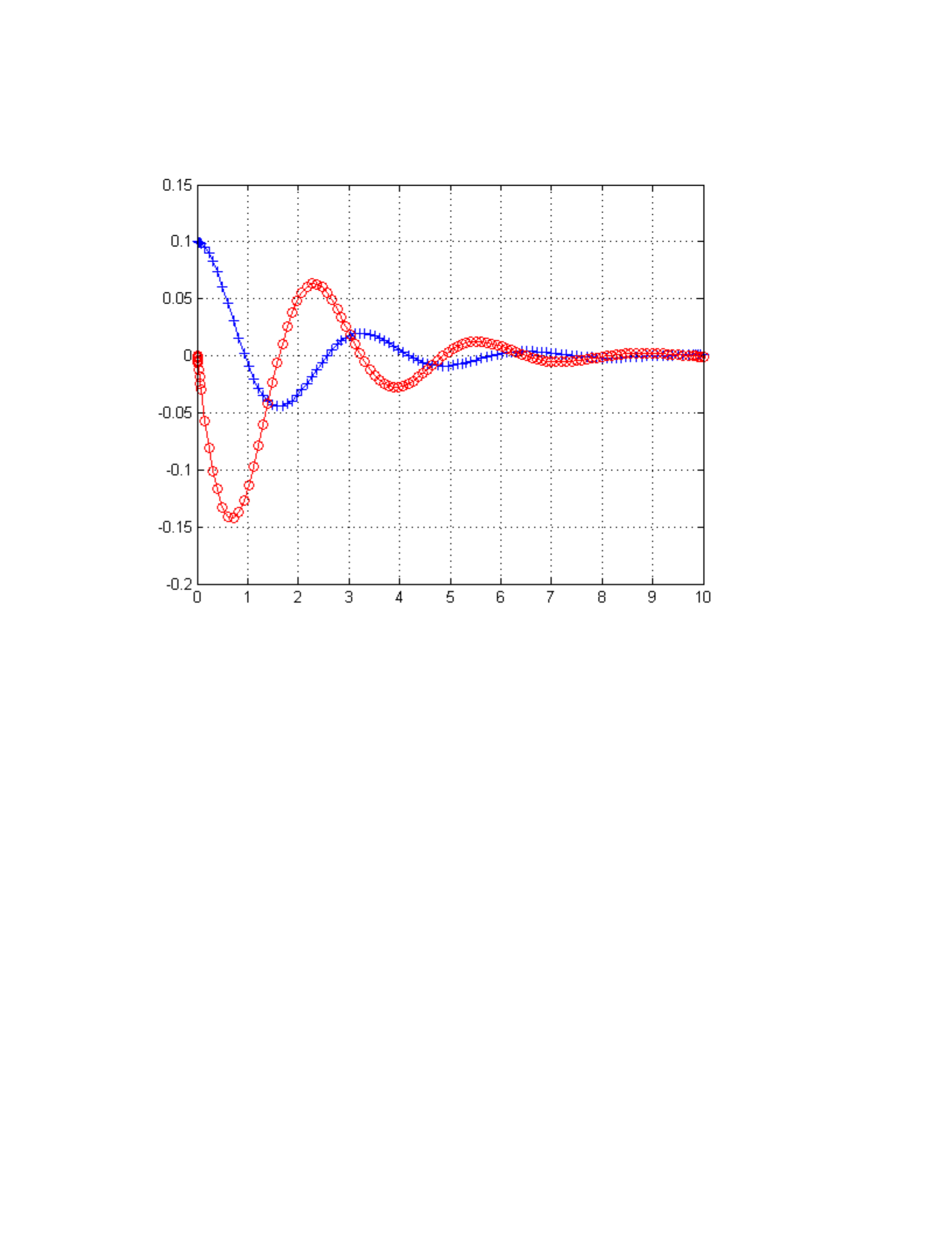
The value we are looking for is 0.1 on the blue curve. Using the zoom
feature we can look at the graph and determine this point to occur at around
3.8
Part B
Knowing that the red curve is the velocity we can assume that the
maximum velocity will take place at one of its peaks. Knowing that this is a
damped oscillation these peaks will get smaller and smaller. To obtain the
maximum velocity we must look at the first peak. This peak occurs around 0.7
seconds. And the magnitude is roughly -0.14
Part C
Knowing that c is our damping constant we will assume that as c
increased, our curve will become more and more damped till it is critically
damped and finally over damped.
function LAB05ex1a
m = 1; % mass [kg]
k = 4; % spring constant [N/m]
c = 2; % friction coefficient [Ns/m]
omega0 = sqrt(k/m); p = c/(2*m);
y0 = 0.1; v0 = 0; % initial conditions
[t,Y] = ode45(@f,[0,10],[y0,v0],[],omega0,p); % solve for 0<t<10
y = Y(:,1); v = Y(:,2); % retrieve y, v from Y
figure(1); plot(t,y,'b+-',t,v,'ro-'); % time series for y and v
grid on;
%-------------------------------------------
function dYdt = f(t,Y,omega0,p)
y = Y(1); v = Y(2);
dYdt = [ v ; -omega0^2*y-2*p*v ]; % fill-in dv/dt
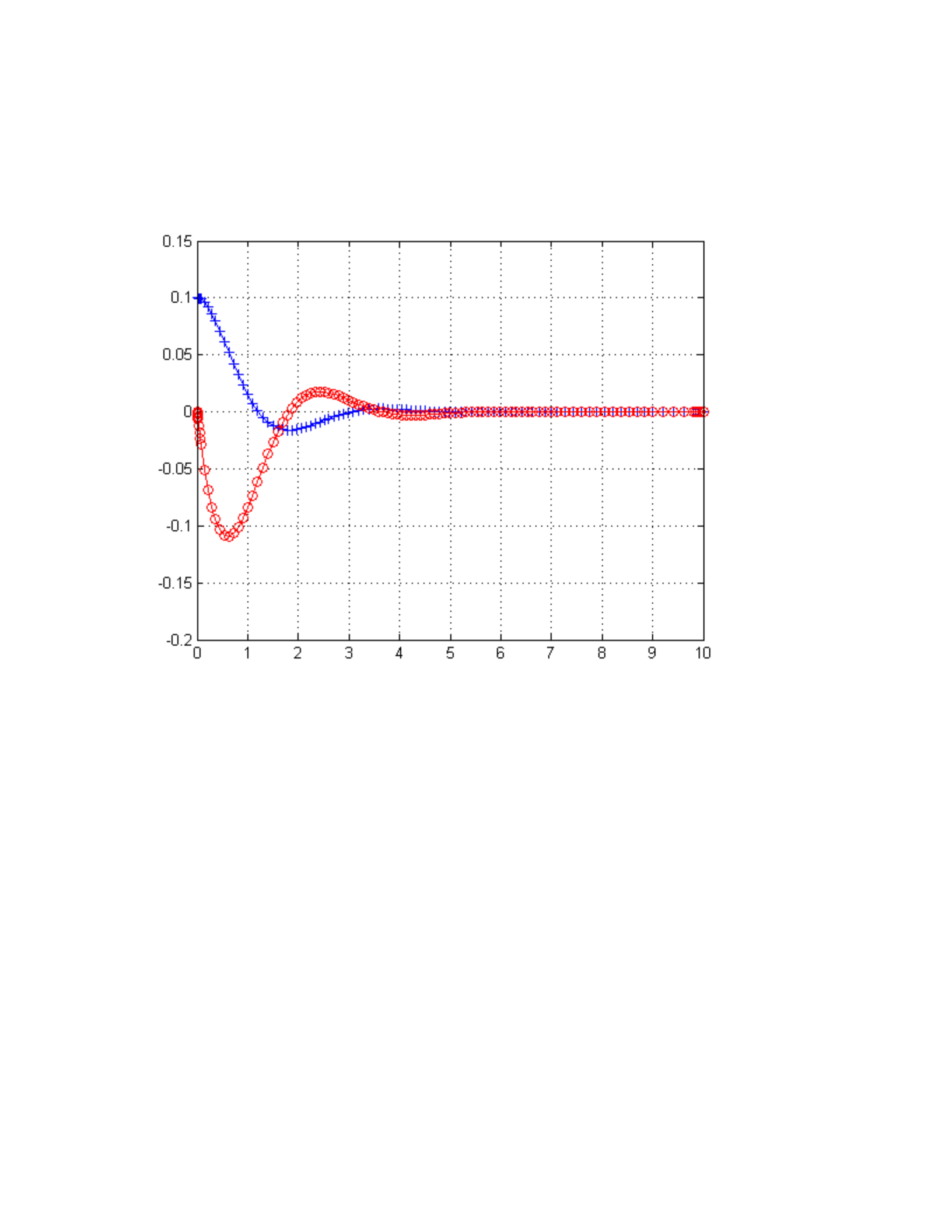
C=2
Looking at this graph we see that there are still two oscillations before the
weight reached equilibrium meaning that this system is under damped.
function LAB05ex1a
m = 1; % mass [kg]
k = 4; % spring constant [N/m]
c = 4; % friction coefficient [Ns/m]
omega0 = sqrt(k/m); p = c/(2*m);
y0 = 0.1; v0 = 0; % initial conditions
[t,Y] = ode45(@f,[0,10],[y0,v0],[],omega0,p); % solve for 0<t<10
y = Y(:,1); v = Y(:,2); % retrieve y, v from Y
figure(1); plot(t,y,'b+-',t,v,'ro-'); % time series for y and v
grid on;
%-------------------------------------------
function dYdt = f(t,Y,omega0,p)
y = Y(1); v = Y(2);
dYdt = [ v ; -omega0^2*y-2*p*v ]; % fill-in dv/dt
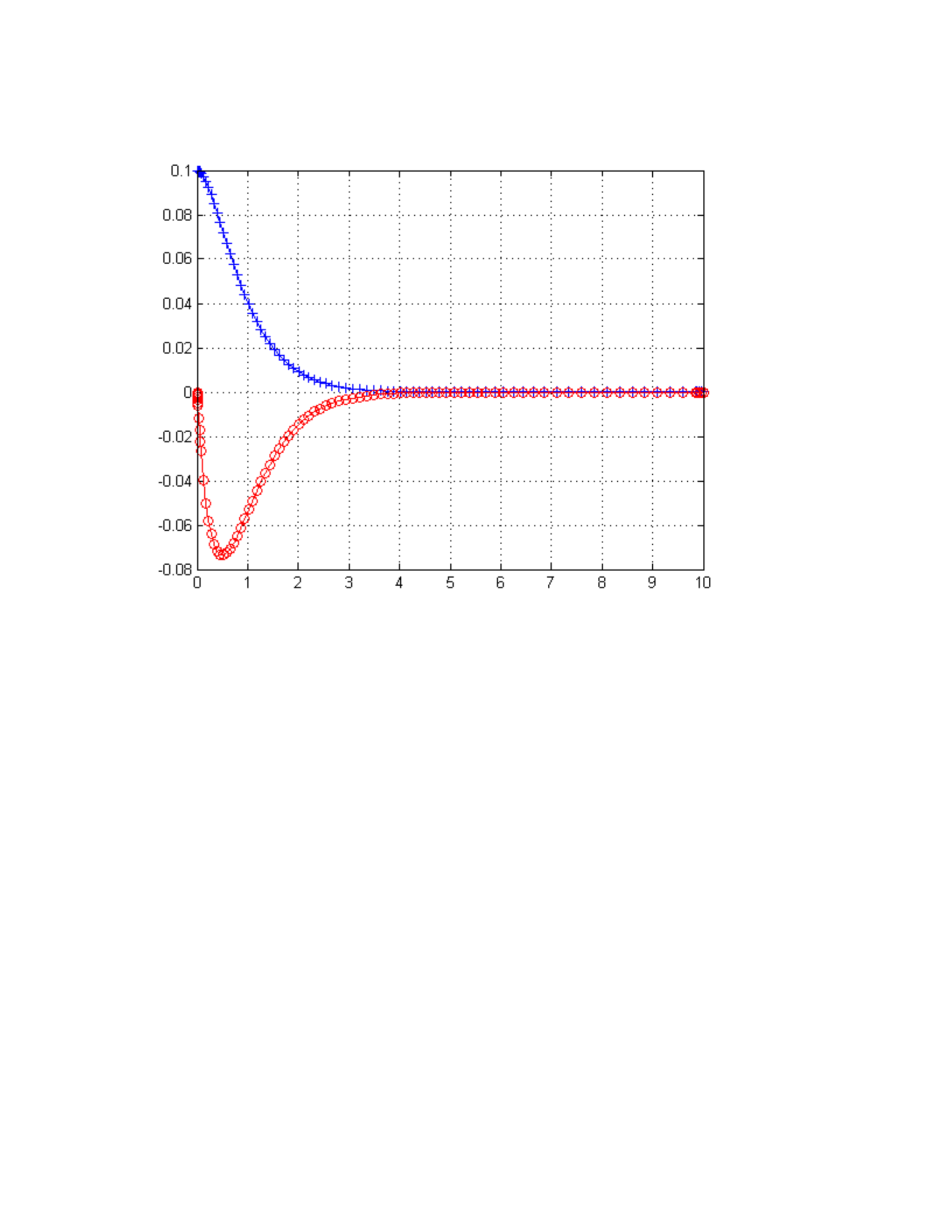
C=4
Looking at this graph we see that there are no oscillations and the system
makes it back to equilibrium around four seconds. With no oscillations we can
assume that this system is critically damped.
function LAB05ex1a
m = 1; % mass [kg]
k = 4; % spring constant [N/m]
c = 6; % friction coefficient [Ns/m]
omega0 = sqrt(k/m); p = c/(2*m);
y0 = 0.1; v0 = 0; % initial conditions
[t,Y] = ode45(@f,[0,10],[y0,v0],[],omega0,p); % solve for 0<t<10
y = Y(:,1); v = Y(:,2); % retrieve y, v from Y
figure(1); plot(t,y,'b+-',t,v,'ro-'); % time series for y and v
grid on;
%-------------------------------------------
function dYdt = f(t,Y,omega0,p)
y = Y(1); v = Y(2);
dYdt = [ v ; -omega0^2*y-2*p*v ]; % fill-in dv/dt
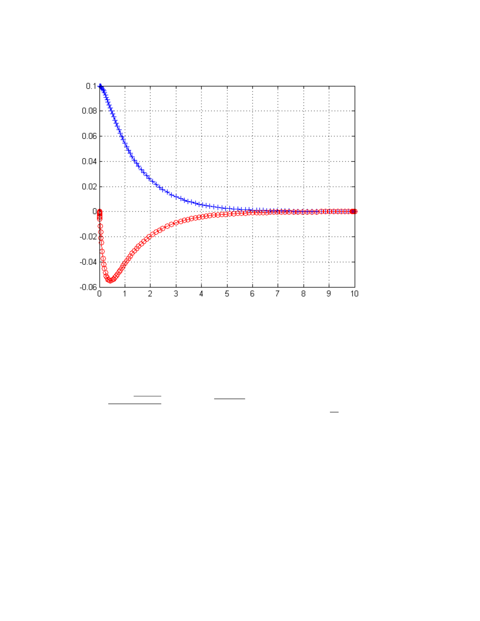
C=6
Looking at this graph we see that the system barely makes it back to
equilibrium at around 8.6 seconds with no oscillations. This leads us to
assume that this system is over damped.
Part D
The critical value of c is obtained by requiring that the characteristic
equation has a repeated root.
Our characteristic equation has the form:
𝑟2+ 2𝑝𝑟 + 𝜔02= 0
Roots: r = −2𝑝+/−√4𝑝2−4𝜔02
2 = -p +/- √𝑝2− 𝜔02
The characteristic equation only has repeated roots when √16. This means the
critical point is c = 4. This agrees with the graph that we got above.
Exercise #4
Part A
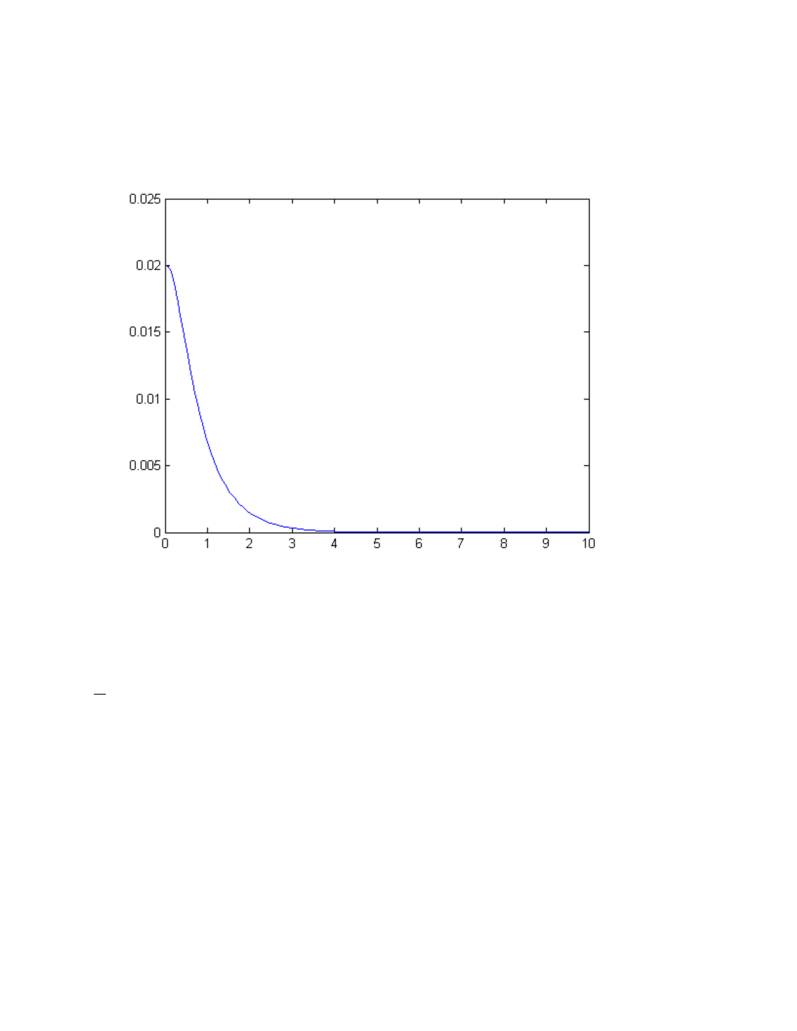
Plotting the quantity E:
function LAB05ex1a
m = 1; % mass [kg]
k = 4; % spring constant [N/m]
c = 6; % friction coefficient [Ns/m]
omega0 = sqrt(k/m); p = c/(2*m);
y0 = 0.1; v0 = 0; % initial conditions
[t,Y] = ode45(@f,[0,10],[y0,v0],[],omega0,p); % solve for 0<t<10
y = Y(:,1); v = Y(:,2); % retrieve y, v from Y
figure(1); plot(t,y,'b+-',t,v,'ro-'); % time series for y and v
grid on;
E=m*v.^2/2+k*y.^2/2
figure(2); plot(t,E)
%-------------------------------------------
function dYdt = f(t,Y,omega0,p)
y = Y(1); v = Y(2);
dYdt = [ v ; -omega0^2*y-2*p*v ]; % fill-in dv/dt
We can see by looking at the curve that energy is not conserved. This system
quickly loses its energy in roughly 4 seconds. ‘
Part B
From the Differential Equation we have the following equation.
v’ = y’’ = -𝜔02𝑦 = -(k/m)y
We then have:
𝑑𝐸
𝑑𝑡 = 1/2 m2vv’ + 1/2 k2yy’
= mvv’ + kyy’
= my’(-k/m)y + kyy’ = 0
Part C
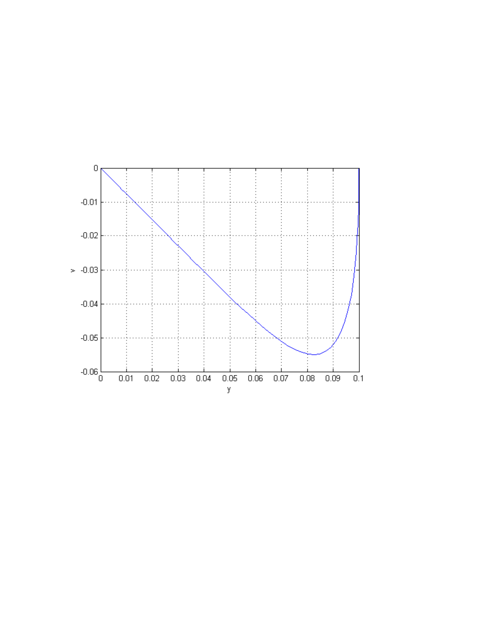
Plotting the phase plot:
function LAB05ex1a
m = 1; % mass [kg]
k = 4; % spring constant [N/m]
c = 6; % friction coefficient [Ns/m]
omega0 = sqrt(k/m); p = c/(2*m);
y0 = 0.1; v0 = 0; % initial conditions
[t,Y] = ode45(@f,[0,10],[y0,v0],[],omega0,p); % solve for 0<t<10
y = Y(:,1); v = Y(:,2); % retrieve y, v from Y
figure(1); plot(t,y,'b+-',t,v,'ro-'); % time series for y and v
grid on;
E=m*v.^2/2+k*y.^2/2
figure(2); plot(t,E);
figure(3)
plot(y,v);
xlabel('y'); ylabel ('v'); grid on
%-------------------------------------------
function dYdt = f(t,Y,omega0,p)
y = Y(1); v = Y(2);
dYdt = [ v ; -omega0^2*y-2*p*v ]; % fill-in dv/dt
This graph is a curve. The maximum value of y is 0.1 and the minimum is 0.
The maximum value of the velocity is -0.054 and the minimum is 0. The curve
starts at the origin and at 0.1 returns to 0 on the x axis.

