



MAT 275 MATLAB LAB 5 NAME:
LAB DAY and TIME:
Instructor:
Exercise 1
Part a)
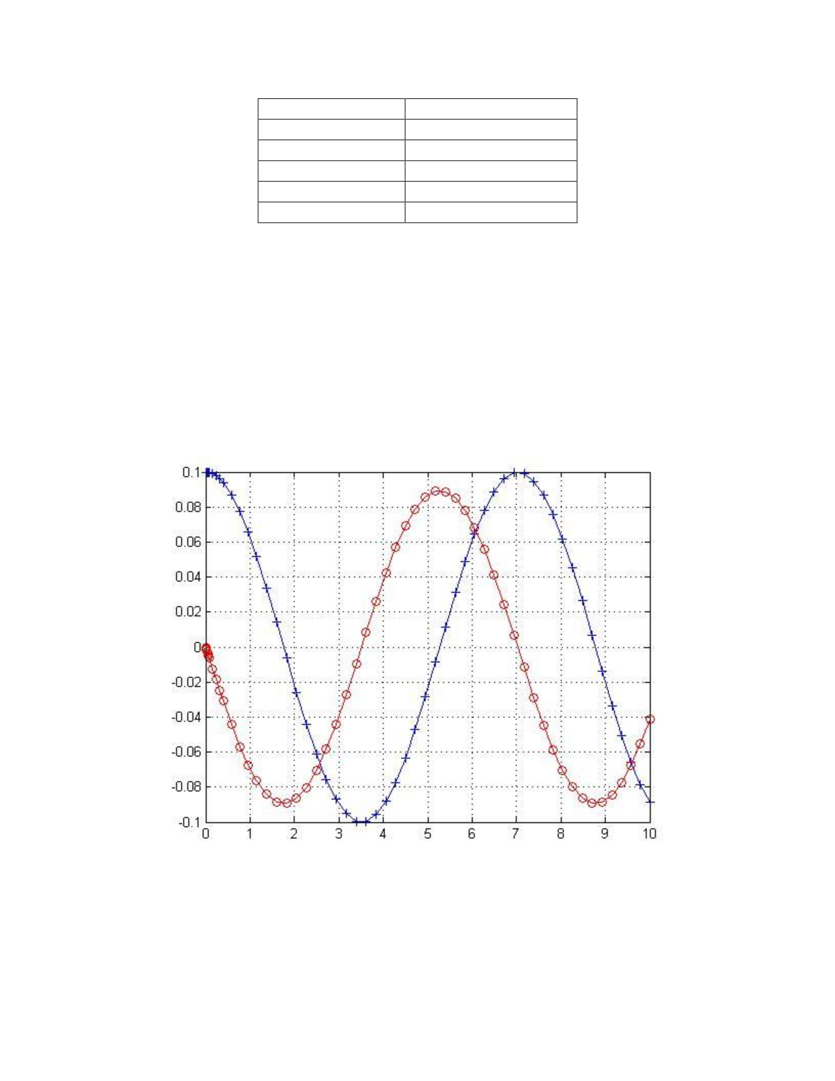
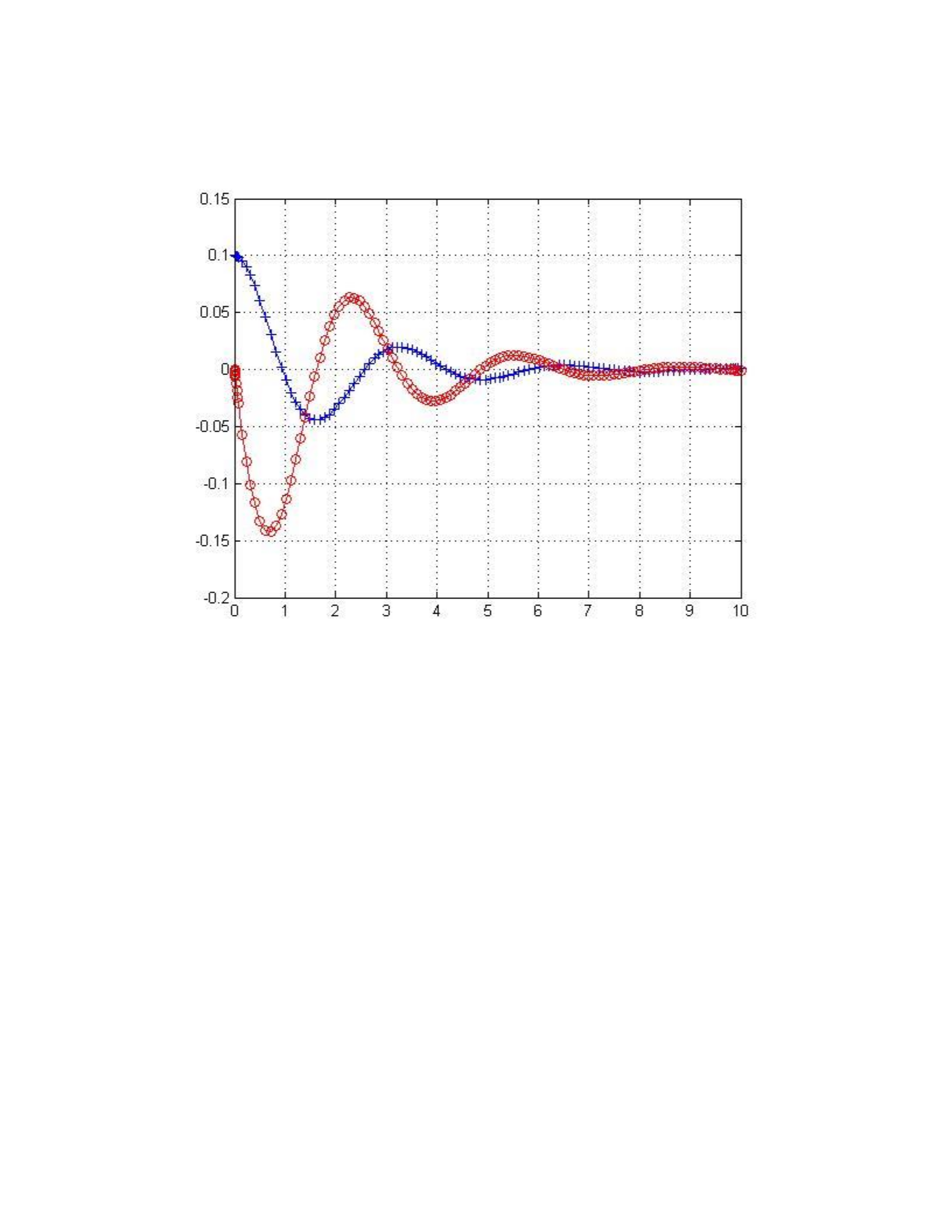
The curve in blue (with ‘+’ symbols) represents the equation y = y(t). The fact that it starts from
a non-zero initial value makes it clear that the mass-spring system is displaced by some initial
displacement – which is given by y. Also the other curve in red (with ‘o’ symbols) starts from
origin indicating the spring is at rest (null velocity) at t = 0 – which represents velocity or y’(t).
Part b)
The period of a typical “sine” wave is the time taken in completing one full cycle. For the curve
y = y(t) (in red) it is approximately equal to 3.1 s.
Since ω = 2 rad/s, the time period T is given by the following equation:
T = 2π/ω
Putting ω = 2, we get T ≈ 3.1 s (which agrees with the value obtained graphically).
Part c)
Ideally, the mass should not come to a rest (if the spring is assumed to be ideal – there are no
damping factors which oppose the motion of the mass). If there are no other forces (friction
force due to air, damping forces) the mass would continue to oscillate without coming to a rest.
If we consider the damping forces (that is the spring damping factor is not equal to zero)
the mass will come to rest after certain period of time depending on the damping forces and
the damping factor. In the real world there will be some damping forces thus, the spring would
eventually come to a rest after certain oscillations.
Part d)
The maximum amplitude of the oscillations of ‘y’ is equal to 0.1 m (the initial displacement of
the mass). The mass continues to oscillate between ±0.1 m (where ‘-‘ indicates negative
direction).
Part e)
The maximum velocity attained by the mass is ≈ 0.99 m/s. It occurs at the extreme positions i.e.
when the amplitude of the displacement is maximum. The following table shows the time
instances at which the maximum velocity occurs:
Time (s)
Velocity (m/s)
2.3904
0.1995
3.9415
-0.1999
5.4479
0.1990
7.0329
-0.1995
8.6095
0.1996
Table – Instances where max velocity occurs
Part f)
The relation between ω, k and m is:
ω 2 = k/m
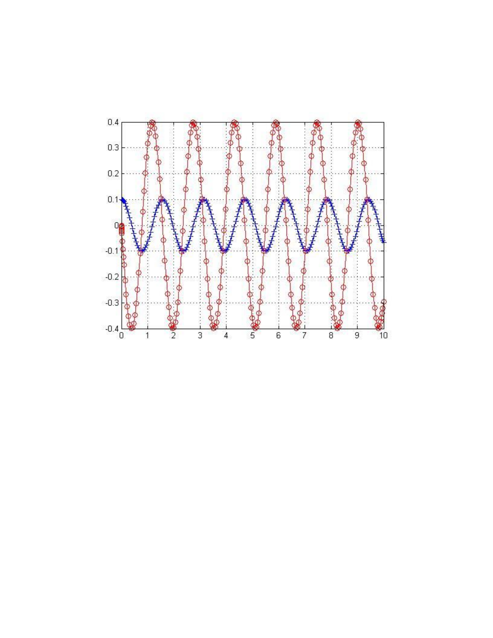
Clearly, the period of oscillation is dependent on both k and m. As m is increased the time
period (T = 2π/ω) increases as ω decreases by a factor of 1/m0.5. The following graph illustrates
the scenario where k = 4 and m = 5 (was earlier equal to 4):
Figure – Increasing m
On the contrary, as k is increased the time period (T) decreases. The natural frequency ω is
increased by a factor of k0.5. The graph below shows the time period when m = 1 and k = 16
(increased from 4 to 16):
Figure – Increasing k
Exercise 2:
Part a)
On plotting the quantity E = ½ mv2 + ½ ky2 we see that the Energy is a constant value ≈ 0.02
units and is independent of ‘t’. Since the energy comes out to be a constant this proves the fact
that the energy is conserved at all times (spring potential energy and kinetic energy). This is
confirmed by the plot shown below:
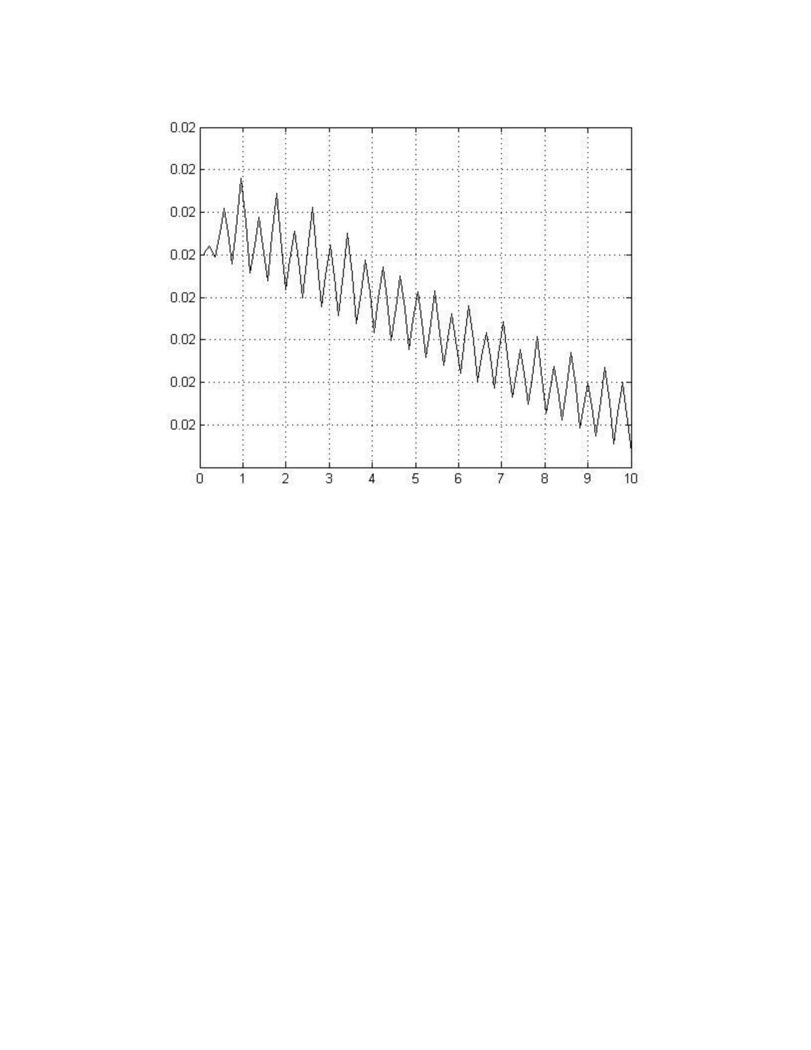
Figure: E vs t (no scaling)
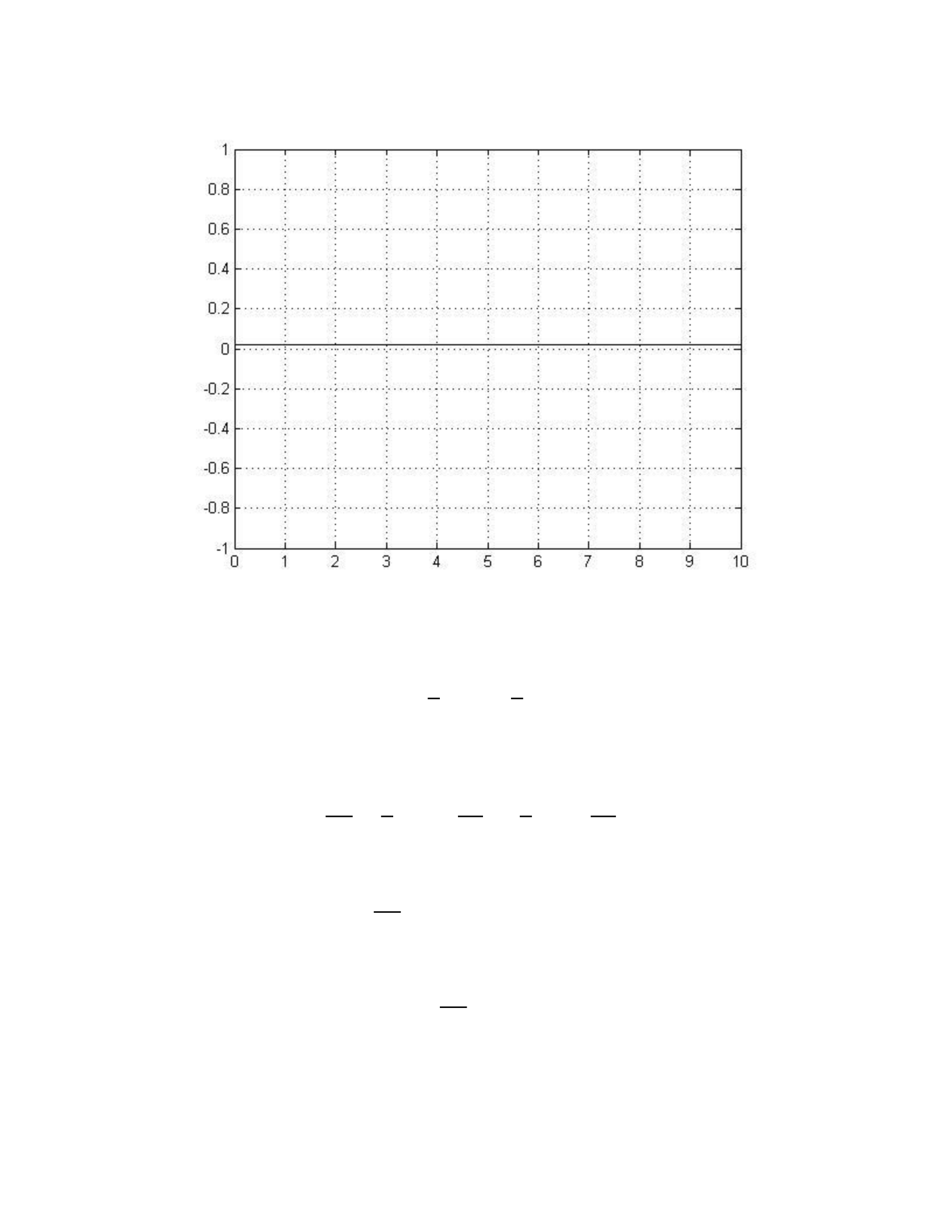
Figure – E vs t (with y limits)
Part b)
𝐸 = 1
2𝑚𝑣2+1
2𝑘𝑦2
Differentiating with respect to time
𝑑𝐸
𝑑𝑡 =1
2𝑚(2𝑣𝑑𝑣
𝑑𝑡)+1
2𝑘(2𝑣𝑑𝑦
𝑑𝑡)
(dy/dt = v and dv/dt = g)
𝑑𝐸
𝑑𝑡 = 𝑣{𝑚(𝑔)+𝑘(𝑦)}
Using the equation L5.2 we get,
𝑑𝐸
𝑑𝑡 = 0
Hence, the energy is constant w.r.t time.
Part c)
Plot:
Figure – Phase Plot (v vs y)
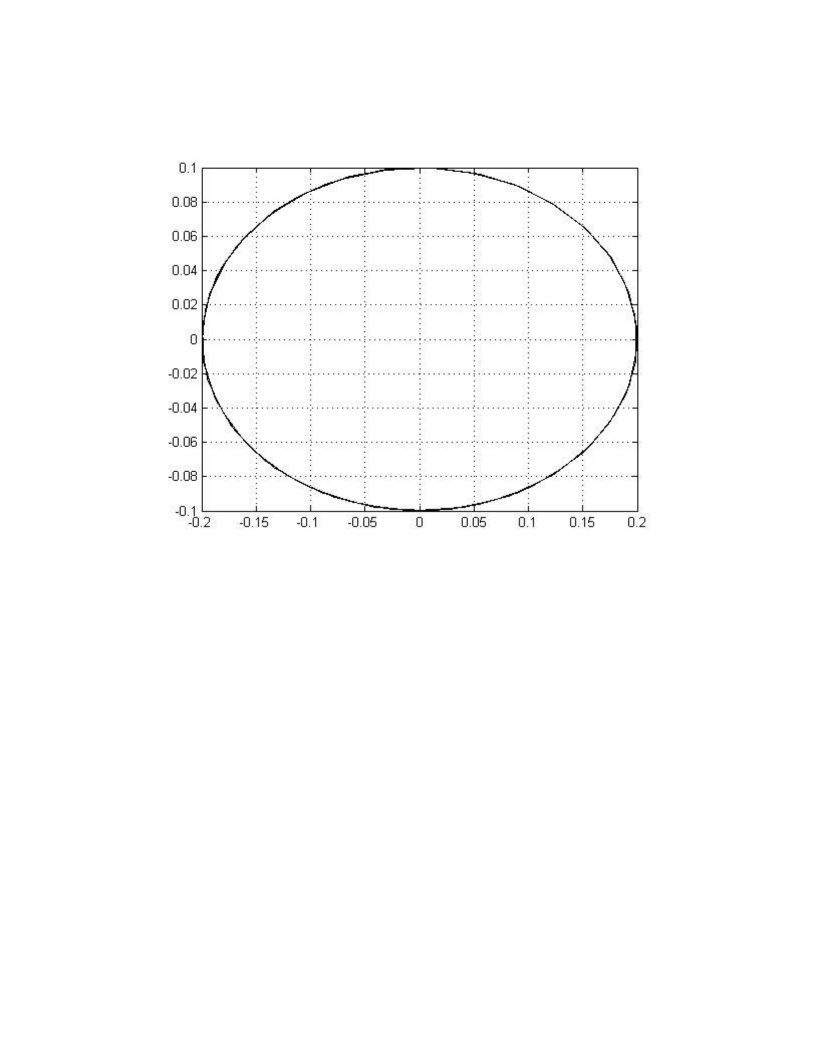
No, the curve never gets closer to the origin. This suggests the fact that the two values are
never zero at the same instant or when the one value is at its minimum from the curve it is
evident that at that point the other value is at its maximum. This confirms the fact that the
velocity is zero when the displacement is maximum and when the velocity is maximum the
displacement is zero. This suggests that the entire kinetic energy gets transformed into spring
potential energy and vice-versa thus, the graph never gets closer to the origin.
Exercise 3
Figure – v(t) (red) and y(t) (blue)
Part a)
On running the modified code the following is printed:
“|y|<0.01 for t>t1 with 3.7807<t1<3.8711”
The code is explained below-
for i=1:length(y)
m(i)=max(abs(y(i:end))); % m(i) contains the maximum displacement
value at each recorded instant
end
i = find(m<0.01); % find returns the indices satisfying the equation
m<0.01 Hence i is a matrix containing all such instances
i = i(1); % to find the first instant where m<0.01 (as this would be
the minimum)
disp(['|y|<0.01 for t>t1 with ' num2str(t(i-1)) '<t1<' num2str(t(i))])
% display the time for which this is true
Part b)
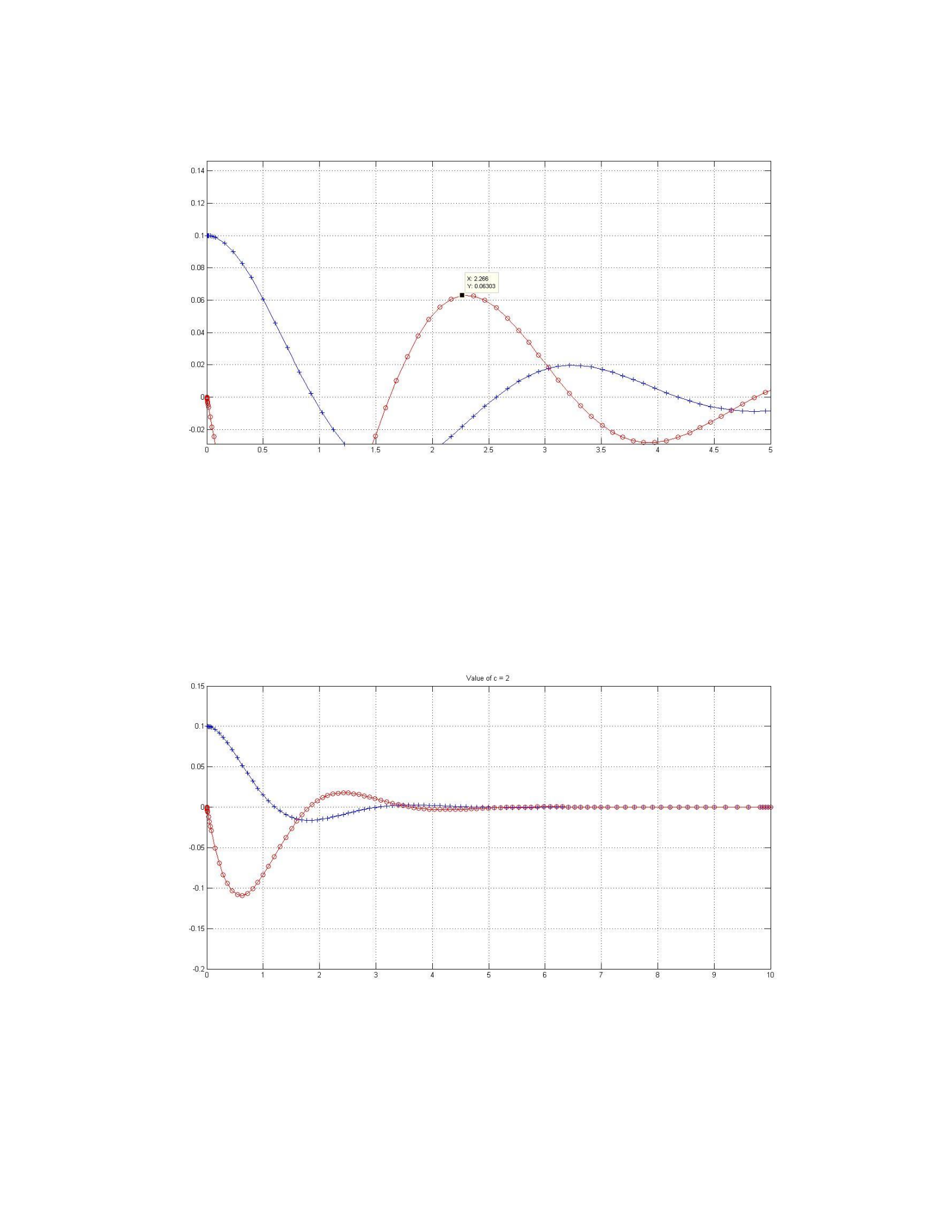
Figure – Maximum Velocity
From the graph it is clear that the maximum velocity is around 0.630 m/s and it occurs around
t = 2.26 s.
Part c)
Graphs depicting the effect of ‘c’ on v(t) and y(t) as the value is increased –
Figure – c = 2
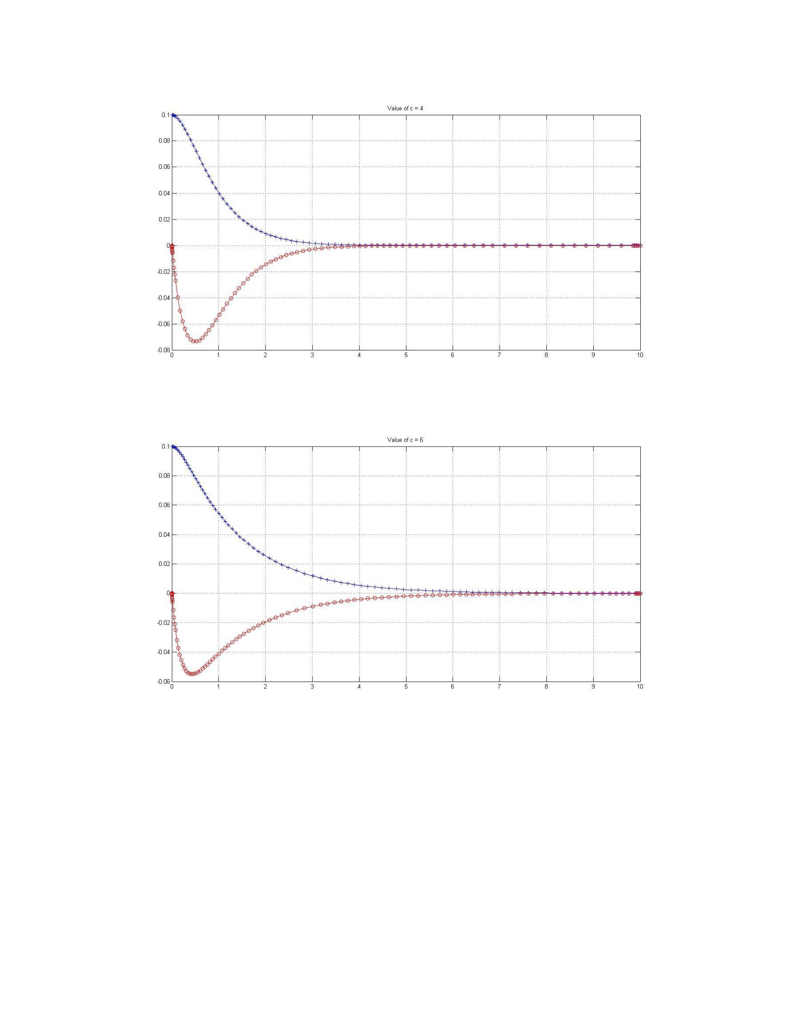
Figure – c = 4
Figure – c= 6
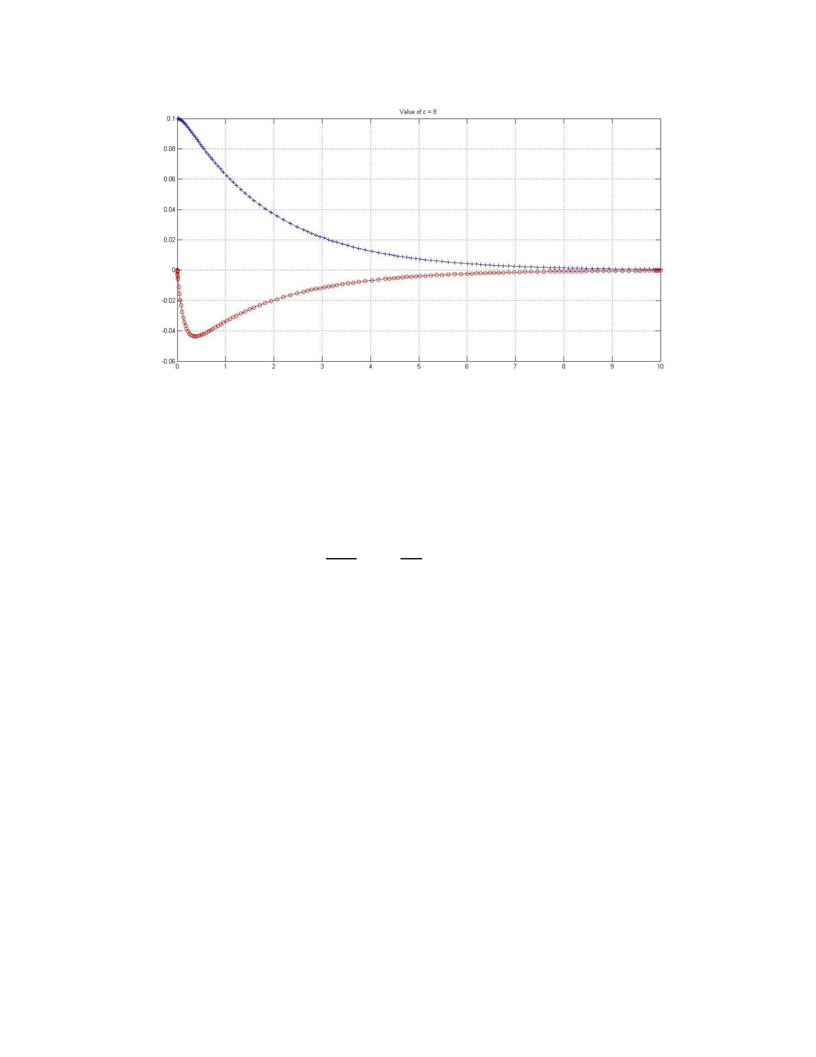
Figure – c= 8
From the graph it becomes quite straightforward to judge that as the value of ‘c’ is increased
the damping forces increases reducing the maximum value attained by the mass and also the
mass comes to rest (stops oscillating) slowly as ‘c’ increases.
Part d)
𝑚𝑑2𝑦
𝑑𝑡2+𝑐(𝑑𝑦
𝑑𝑡)+𝑘𝑦 = 0
With initial conditions:
y(0) = yo, y’(0) = vo
We know that a solution is exponential in nature
y(t) = eλt
Finding the first and second derivative for last expression
y'(t) = λeλt , y’’(t) = λ2eλt
Substituting into the main ODE, we get
(λ2 + 2ᶓω λ + ω2) eλt = 0
By finding the solution for this characteristic equation, the two values of λ are:
λ1,2 = - ᶓω ± ω (ᶓ2 – 1) ½
If the value of ᶓ is equal to 1, two equal negative real roots will result. This corresponds to the
critically damped motion, where the motion is non-oscillatory.
Therefore, when ᶓ = 1, we get c = 2ᶓω . Thus, the minimum value of c where no oscillations
occur is = 4 ( ᶓ = 1 and ω = 2).
Exercise 4
Part a)
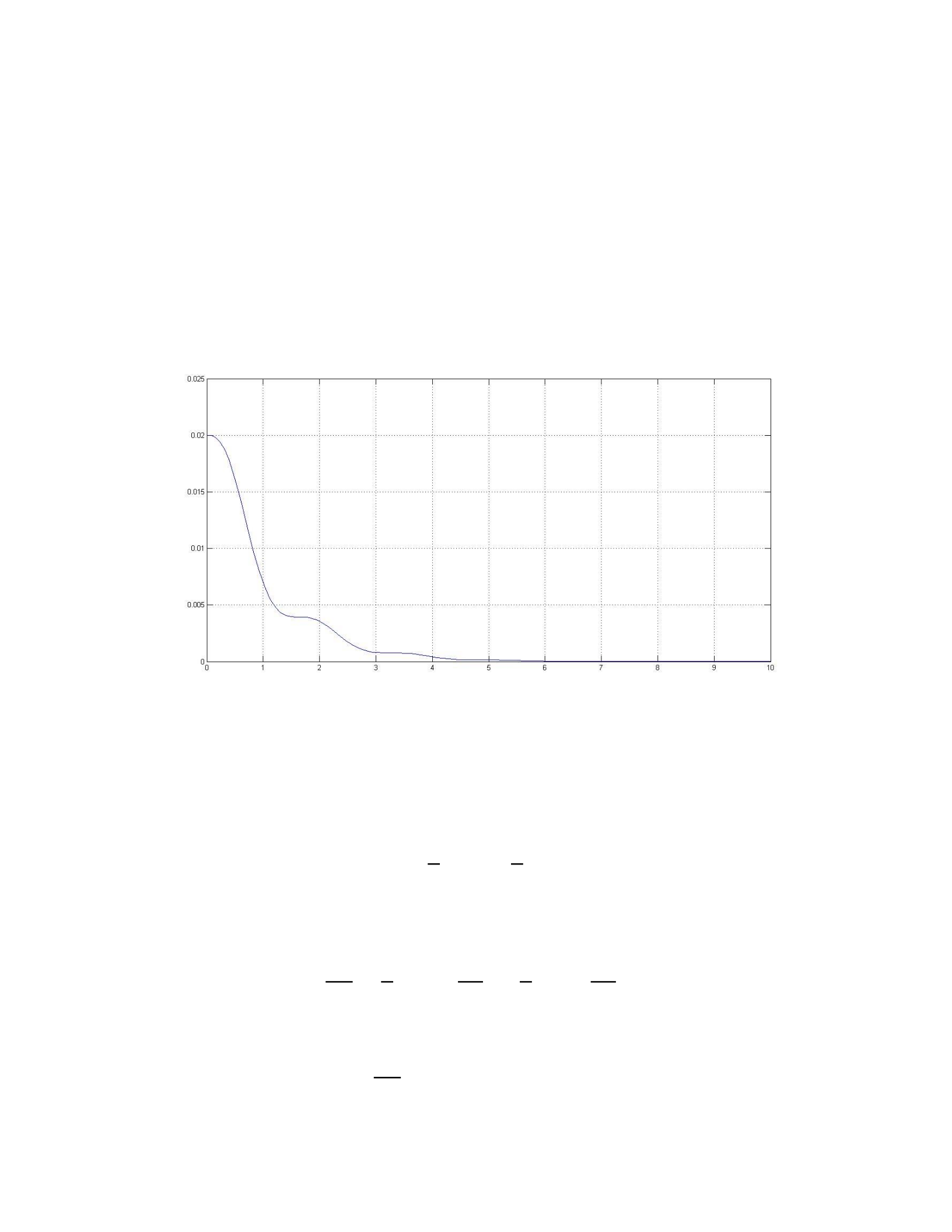
Figure – Energy vs Time
No, the energy is not constant in this case (c = 1) and is therefore not conserved. The energy
function varies in a complex polynomial manner with respect to time.
Part b)
𝐸 = 1
2𝑚𝑣2+1
2𝑘𝑦2
Differentiating with respect to time
𝑑𝐸
𝑑𝑡 =1
2𝑚(2𝑣𝑑𝑣
𝑑𝑡)+1
2𝑘(2𝑣𝑑𝑦
𝑑𝑡)
(dy/dt = v and dv/dt = g)
𝑑𝐸
𝑑𝑡 = 𝑣{𝑚(𝑔)+𝑘(𝑦)}
Using equation L5.4 we get:
𝑑𝐸
𝑑𝑡 = −𝑐𝑣
This clearly shows that when c > 0, dE/dt < 0 and when c <0, dE/dt > 0. Hence proved!
Part c)
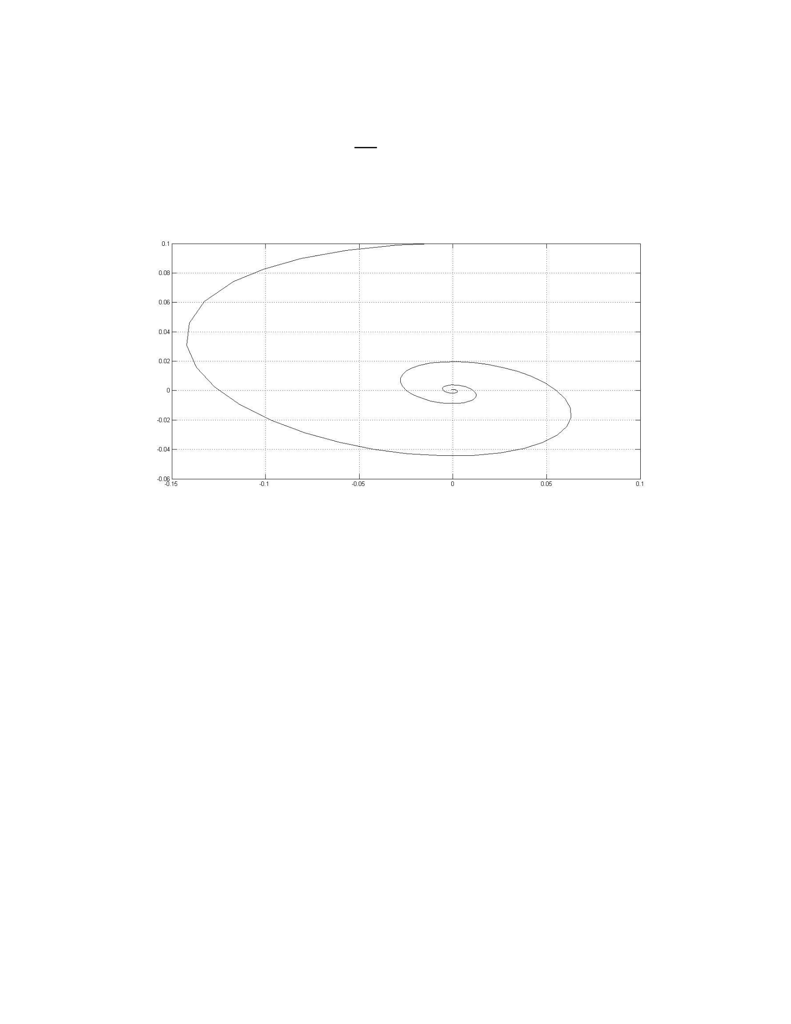
Figure – v vs y
Yes, this time the plot gets close to the origin. This suggests that the energy is not totally
conserved. Hence the entire kinetic energy of the mass is not converted into spring potential
energy (and vice-versa). Due to the damping factors there is a loss in energy and the mass
doesn’t continue to oscillate and finally stops after some time (that is why the curve gets closer
to the origin).

