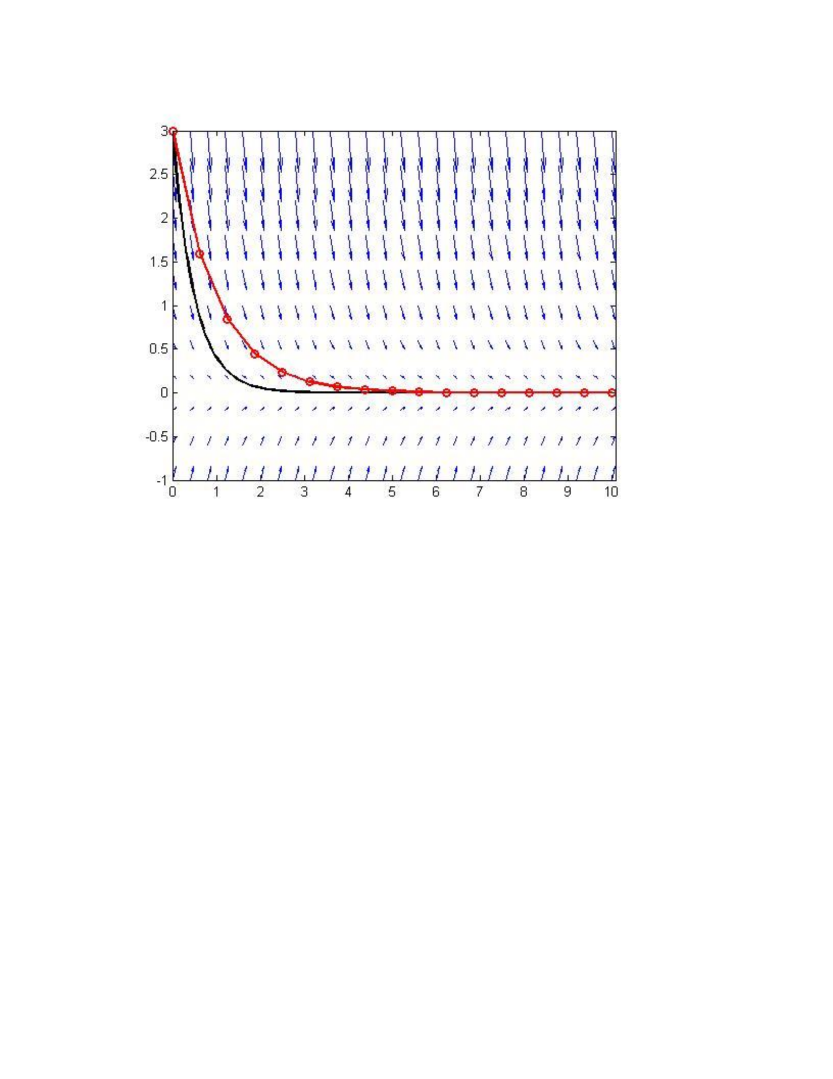
MAT 275 MATLAB LAB 2 NAME:
LAB DAY and TIME:
Instructor:
Exercise 1
Part a)
f=inline('2*y','t','y');
t=linspace(0,.5,100); y=3*exp(2*t); % defines the exact solution of
the ODE
[t5,y5]=euler(f,[0,.5],3, 5); % solves the ODE using Euler with 5
steps
[t50,y50]=euler(f,[0,.5],3, 50); % solves the ODE using Euler with 50
steps
[t500, y500] = euler(f, [0, 0.5], 3, 500); % solves the ODE using
Euler with 500 steps
[t5000, y5000] = euler(f, [0, 0.5], 3, 5000); % solves the ODE using
Euler with 5000 steps
y5(end); % to see the approximate value at t = 0.5 and N = 5
y50(end); % to see the approximate value at t = 0.5 and N = 50
y500(end); % to see the approximate value at t = 0.5 and N = 500
y5000(end); % to see the approximate value at t = 0.5 and N = 5000
% Calculating the errors (exact - approximation) at t=0.5
e5 = y(end) - y5(end); % error with N = 5
e50 = y(end) - y50(end); % error with N = 50
e500 = y(end) - y500(end); % error with N = 500
e5000 = y(end) - y5000(end); % error with N = 5000
% Ratio of the errors:
ratio50 = e5/e50;
ratio500 = e50/e500;
ratio5000 = e500/e5000;
Table:
N
Approximation
Error
ratio
5
7.4650
0.6899
-
50
8.0748
0.0801
8.6148
500
8.1467
0.0081
9.8381
5000
8.1540
8.1534e-04
9.9835
Part b)
The last column is shown below:
ratio
-
8.6148
9.8381
9.9835
The ratio of the errors seems to increase suggesting that the errors are decreasing as the step
size (or the value of N is increased) is decreased. The value of ratio is way too less which
explains the fact that Euler method gives a highly approximate value of the function (though
this value is dependent on ‘h’). But with h being as low as 10-4 the ratio with the previous error
value at h = 10-3 still seems to be only ~10 which is not that a good approximate.
The ratio of consecutive errors increases as the step size is increased. Also from the errors
column we can make out that as the step size is decreased by a factor of 10, the error is also
reduced (approximately) by the same factor. This suggests that the Euler’s method is “of order
h” where h is the step size.
Part c)
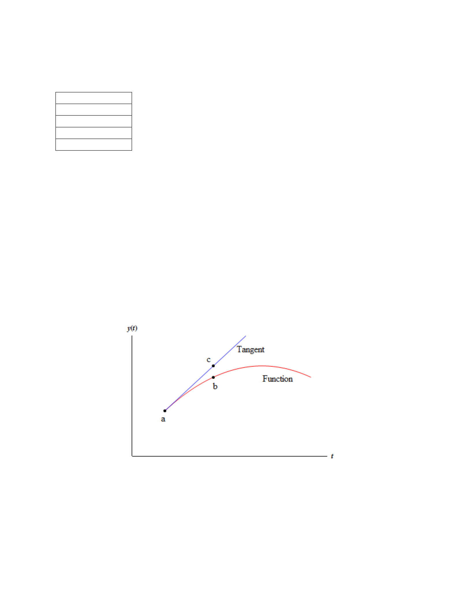
Consider the graph below. It shows a tangent line to a curve at Point a.
If point c is close enough to point a then the points on the tangent line should be fairly close to
the actual value of the function. Similarly, in the euler method we start at some point and then
start moving to a point closer to the actual curve depending on the step size. We continue
doing this till all the steps are covered. Thus, the values which are obtained approximate the
value of the function but there is some errors in the values as it depends on the step size or the
number of steps.
Exercise 2:
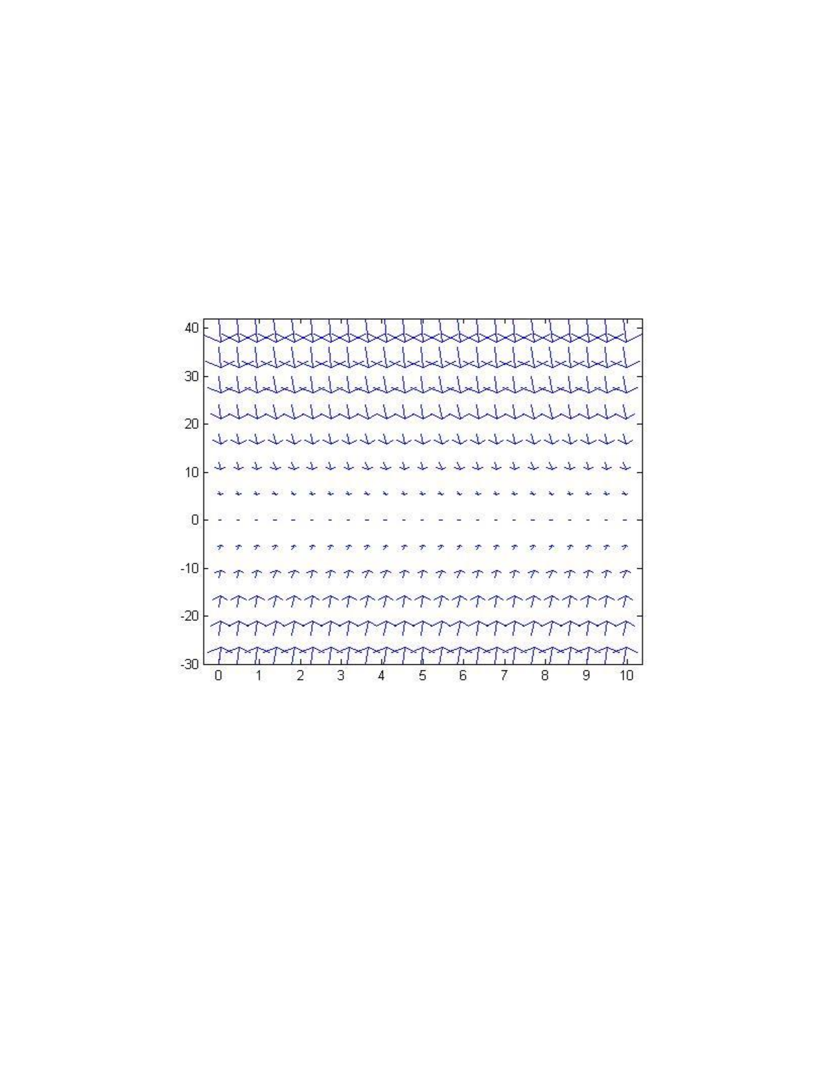
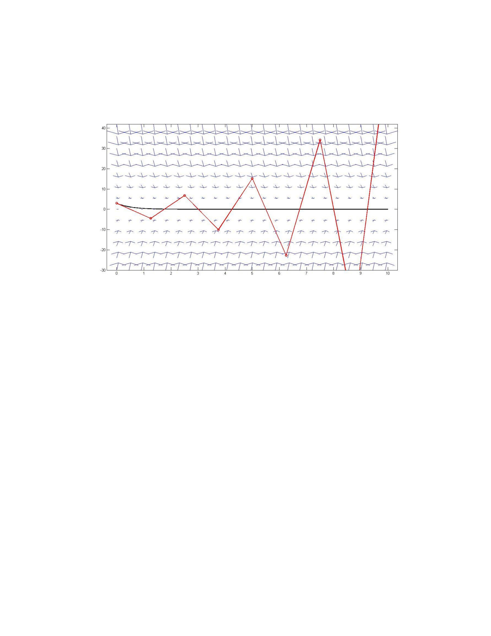
% Part A
t=0:.45:10; y = -30:6:42;
[T,Y]=meshgrid(t,y);
dT=ones(size(T));
dY= -2*Y;
quiver(T,Y,dT,dY)
axis tight
hold on
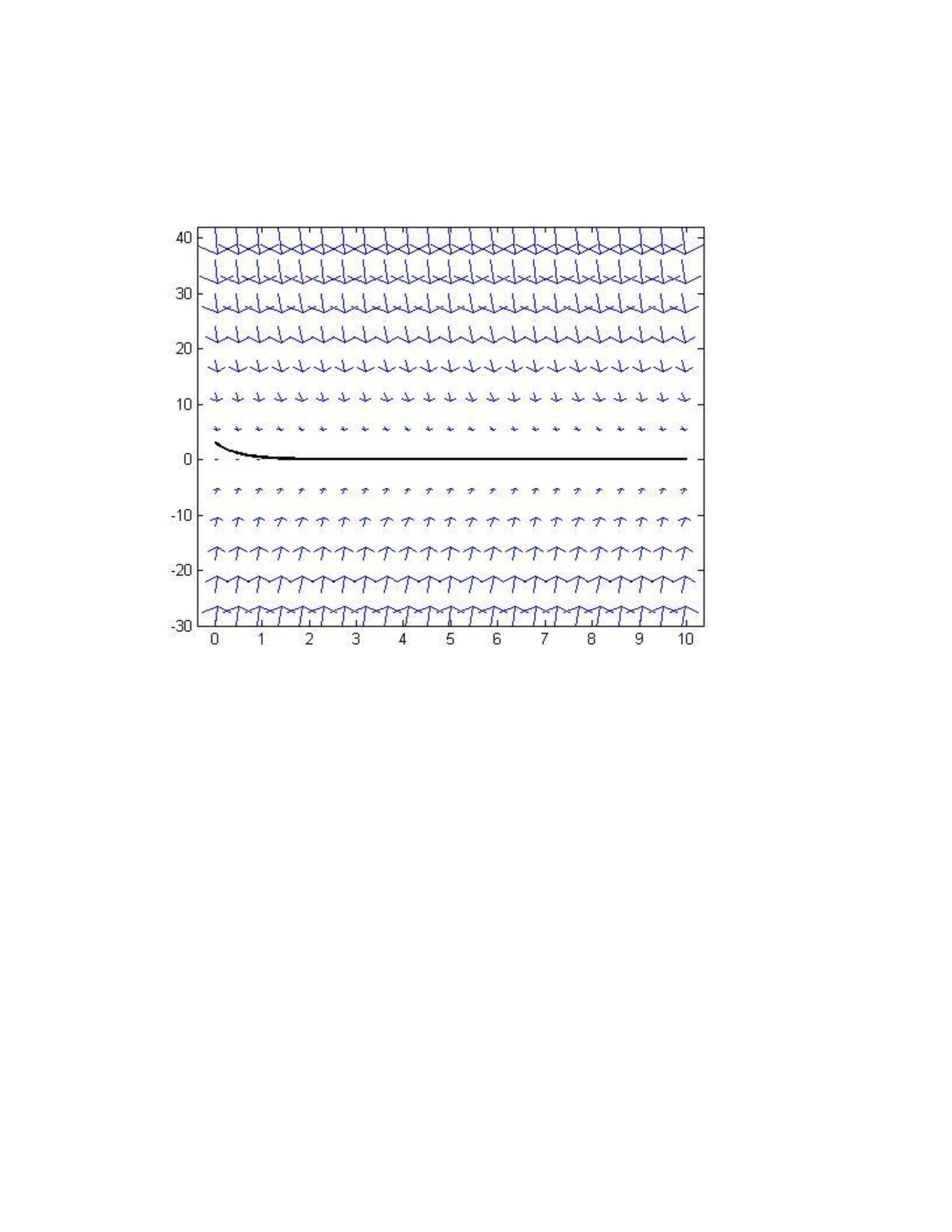
% Part B
t = linspace(0, 10, 200);
y = 3.*exp(-2.*t);
plot(t, y, 'k', 'LineWidth', 2);
% Part C
f = inline('-2*y','t','y');
[t, y] = euler(f, [0, 10], 3, 8);
plot(t, y, 'ro-', 'LineWidth', 2);
% Part D
figure
t=0:.4:10; y = -1:0.4:3;
[T,Y]=meshgrid(t,y);
dT=ones(size(T));
dY= -2*Y;
quiver(T,Y,dT,dY)
axis tight
hold on
t = linspace(0, 10, 200);
y = 3.*exp(-2.*t);
plot(t, y, 'k', 'LineWidth', 2);
f = inline('-2*y','t','y');
[t, y] = euler(f, [0, 10], 3, 16);
plot(t, y, 'ro-', 'LineWidth', 2);

Improved Euler function (impeuler.m)
function [t,y] = impeuler(f,tspan,y0,N)
% Solves the IVP y’ = f(t,y), y(t0) = y0 in the time interval tspan =
[t0,tf]
% using Improved Euler’s method with N time steps.
% Input:% f = name of inline function or function M-file that
evaluates the ODE
% (if not an inline function, use: impeuler(@f,tspan,y0,N))
% For a system, the f must be given as column vector.
% tspan = [t0, tf] where t0 = initial time value and tf = final time
value
% y0 = initial value of the dependent variable. If solving a system,
% initial conditions must be given as a vector.
% N = number of steps used.
% Output:
% t = vector of time values where the solution was computed
% y = vector of computed solution values.
m = length(y0);
t0 = tspan(1);
tf = tspan(2);
h = (tf-t0)/N; % evaluate the time step size
t = linspace(t0,tf,N+1); % create the vector of t values
y = zeros(m,N+1); % allocate memory for the output y
y(:,1) = y0'; % set initial condition
for n=1:N
f1 = f(t(n), y(:, n));
f2 = f(t(n) + h, y(:, n) + h*f1);
y(:,n+1) = y(:,n) + (h/2)*(f1 + f2); % implement Improved Euler’s
method
end
t = t'; y = y'; % change t and y from row to column vectors
end

Exercise 3
f = inline('2*y','t','y');
[t5,y5] = impeuler(f,[0,.5],3,5);
[t5, y5]
ans =
0 3.0000
0.1000 3.6600
0.2000 4.4652
0.3000 5.4475
0.4000 6.6460
0.5000 8.1081
Exercise 4
Part a)
f=inline('2*y','t','y');
t=linspace(0,.5,100); y=3*exp(2*t); % defines the exact solution of
the ODE
[t5,y5]= impeuler(f,[0,.5],3, 5); % solves the ODE using Improved
Euler with 5 steps
[t50,y50]= impeuler(f,[0,.5],3, 50); % solves the ODE using Improved
Euler with 50 steps
[t500, y500] = impeuler(f, [0, 0.5], 3, 500); % solves the ODE using
Improved Euler with 500 steps
[t5000, y5000] = impeuler(f, [0, 0.5], 3, 5000); % solves the ODE
Improved using Euler with 5000 steps
y5(end); % to see the approximate value at t = 0.5 and N = 5
y50(end); % to see the approximate value at t = 0.5 and N = 50
y500(end); % to see the approximate value at t = 0.5 and N = 500
y5000(end); % to see the approximate value at t = 0.5 and N = 5000
% Calculating the errors (exact - approximation) at t=0.5
e5 = y(end) - y5(end); % error with N = 5
e50 = y(end) - y50(end); % error with N = 50
e500 = y(end) - y500(end); % error with N = 500
e5000 = y(end) - y5000(end); % error with N = 5000
% Ratio of the errors:
ratio50 = e5/e50;
ratio500 = e50/e500;
ratio5000 = e500/e5000;

Table:
N
Approximation
Error
ratio
5
8.1081
0.0467
-
50
8.1543
5.3555e-04
87.2394
500
8.1548
5.4284e-06
98.6567
5000
8.1548
5.4357e-08
99.8650
Part b)
The last column is shown below:
Ratio
-
87.2394
98.6567
99.8650
The ratio of the errors seems to increase suggesting that the errors are decreasing as the step
size (or the value of N is increased) is decreased. As compared to simple Euler method this time
the ratio are very high which makes it evident that the approximate value by the improved
euler’s method is very close to the actual value of the solution.
The ratio of consecutive errors increases as the step size is increased. Also from the errors
column we can make out that as the step size is decreased by a factor of 100, the error is also
reduced (approximately) by the same factor. This suggests that the Euler’s method is “of order
h2” where h is the step size.
Exercise 5
Part a)
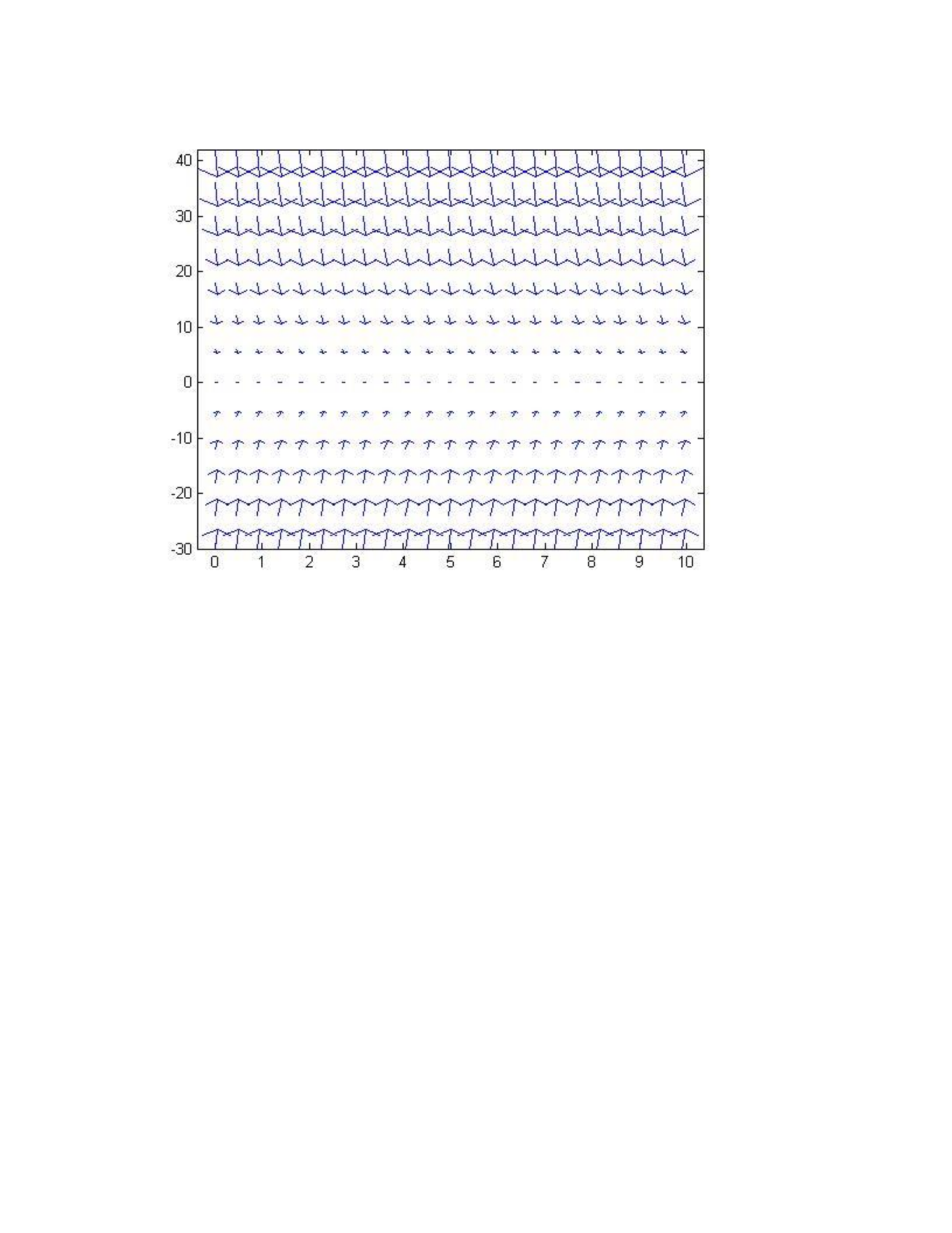
t=0:.45:10; y = -30:6:42;
[T,Y]=meshgrid(t,y);
dT=ones(size(T));
dY= -2*Y;
quiver(T,Y,dT,dY)
axis tight
hold on
Part b)
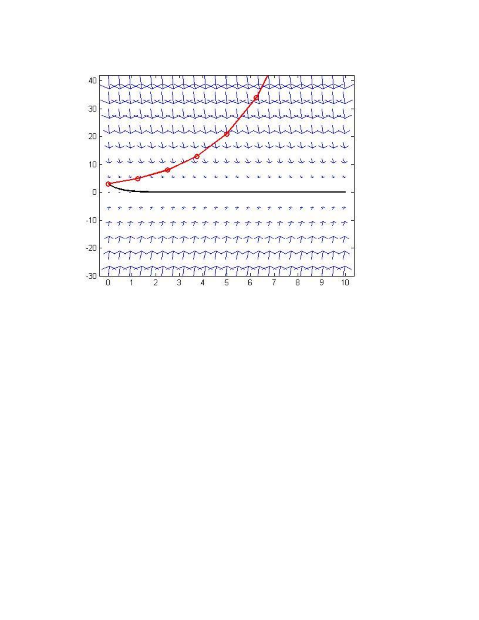
t = linspace(0, 10, 200);
y = 3.*exp(-2.*t);
plot(t, y, 'k', 'LineWidth', 2);

Part c)
f = inline('-2*y','t','y');
[t, y] = impeuler(f, [0, 10], 3, 8);
plot(t, y, 'ro-', 'LineWidth', 2);
Part c)
figure
t=0:.4:10; y = -1:0.4:3;
[T,Y]=meshgrid(t,y);
dT=ones(size(T));
dY= -2*Y;
quiver(T,Y,dT,dY)
axis tight
hold on
t = linspace(0, 10, 200);
y = 3.*exp(-2.*t);
plot(t, y, 'k', 'LineWidth', 2);
f = inline('-2*y','t','y');
[t, y] = impeuler(f, [0, 10], 3, 16);
plot(t, y, 'ro-', 'LineWidth', 2);