



Lab 5 - Zachary Fiveash - MAT 275 Lab
The Mass-Spring System
EX 1
A)
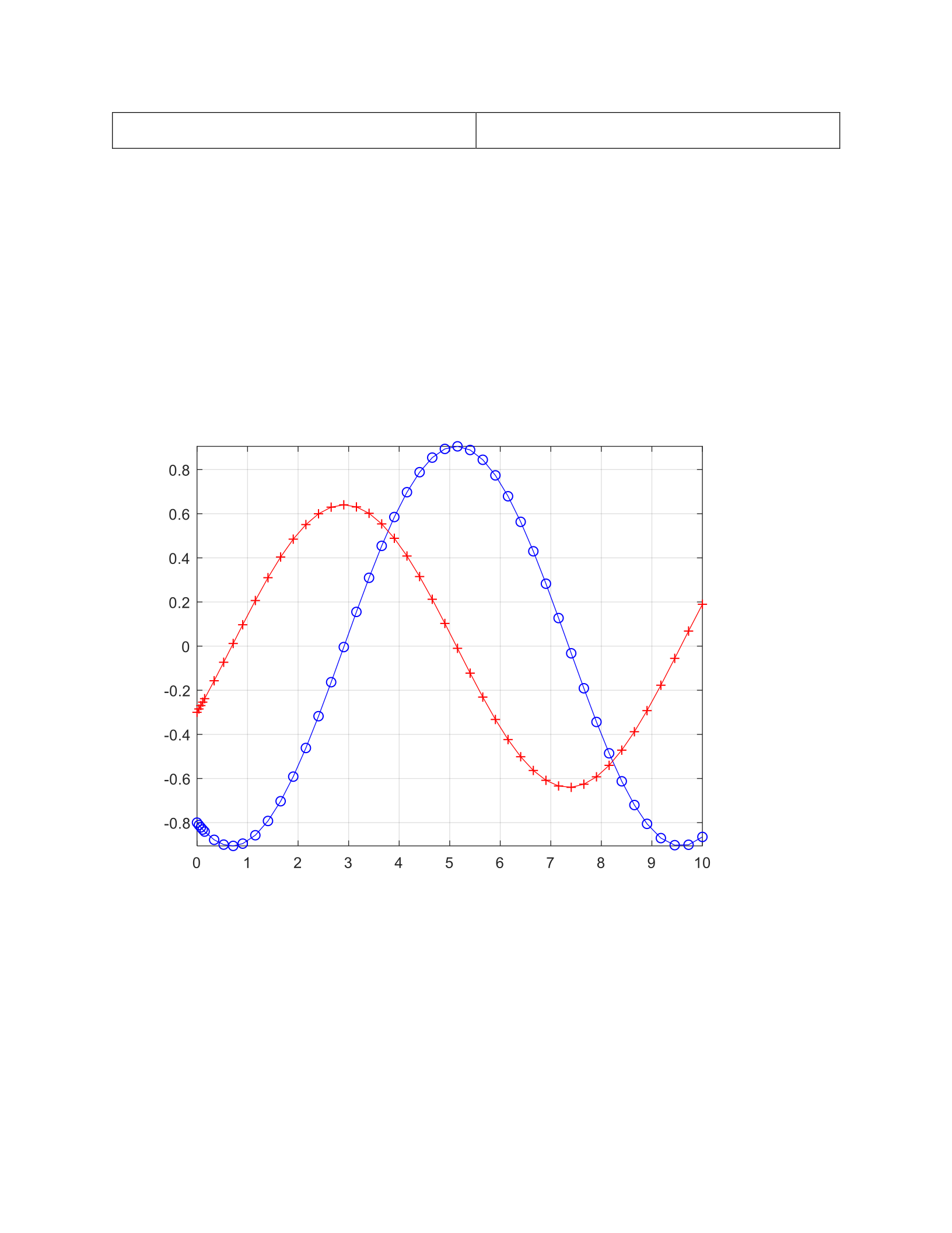
The curve in blue (with 'o' symbols) represents the equation y=y(t). The curve starts from a non-zero
initial value which is a give away that it a mass-spring system is displaced by some initial
displacement: given by y. The other curve in red (with '+' symbols) starts from an origin indicating the
spring is at rest (null velocity) at t = 0; this represents velocity of y'(t).
B)
The curve of y(t) in blue is aproximately equal to 3.097 or 3.1s. Since w=2 rad/s, the time period T is
given by the following equation:
T=2pi/w.
Putting w=2, we get T=3.1s ; which agrees with the value obtained graphically.
C)
Ideally the mass would not come to rest. If the spring is deal as well as all other damping factors that
may oppose the motion of the mass. If there are no other forces such as friction the mass should
oscillate indefinitely. If you take the damping forces into consideration, the mass will come to rest
after a period. A real-world scenario would see the mass eventually come to rest after a period of
oscillation.
D)
The maximum amplitude of oscillation of 'y' is 0.8134.
E)
The maximum velocity attained is 1.628. It occurs at the extreme positions or when the amplitude of
the displacement is maximum.
Time (s)
Velocity (m/s)
0.8778
1.628
2.489
-1.623
4.01
1.627
5.659
-1.612
7.195
1.623
F)
The relationship between 𝜔, k, and m is:
𝜔2= 𝑘/𝑚
The period of oscillation is dependent on k and m. As m is increased the time period increases as
𝜔 decreases. The following graph is of m=8 and k=4.
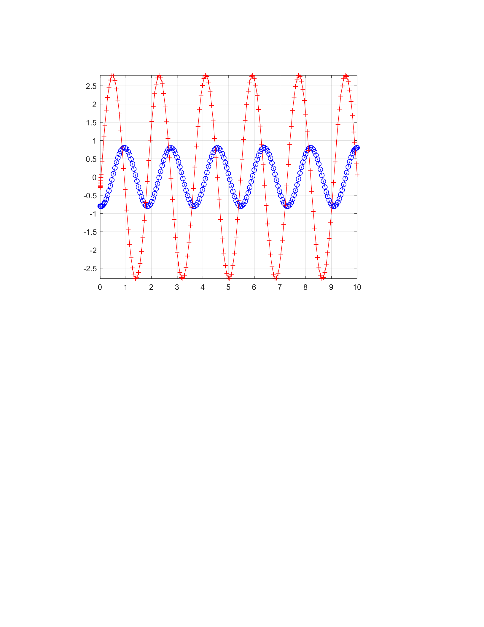
As k is increased the time period decreases. The natural frequency of 𝜔 increases. The graph
above is of m=1 and k=12.
EX 2
A)
clear; close all; clc;
%% parameters
A = 1;
m = 1;
k = 4;
w = sqrt(k/m);
t = linspace(0, 2*pi);
y = A * sin(w*t);
v = A*w * cos(w*t);
%% part (a)
E = .5*m*v.^2 + .5*k*y.^2;
figure
plot(t, E)
xlabel('t')
ylabel('E(t)')
xlim([0 2*pi])
title('Energy vs Time')
grid on
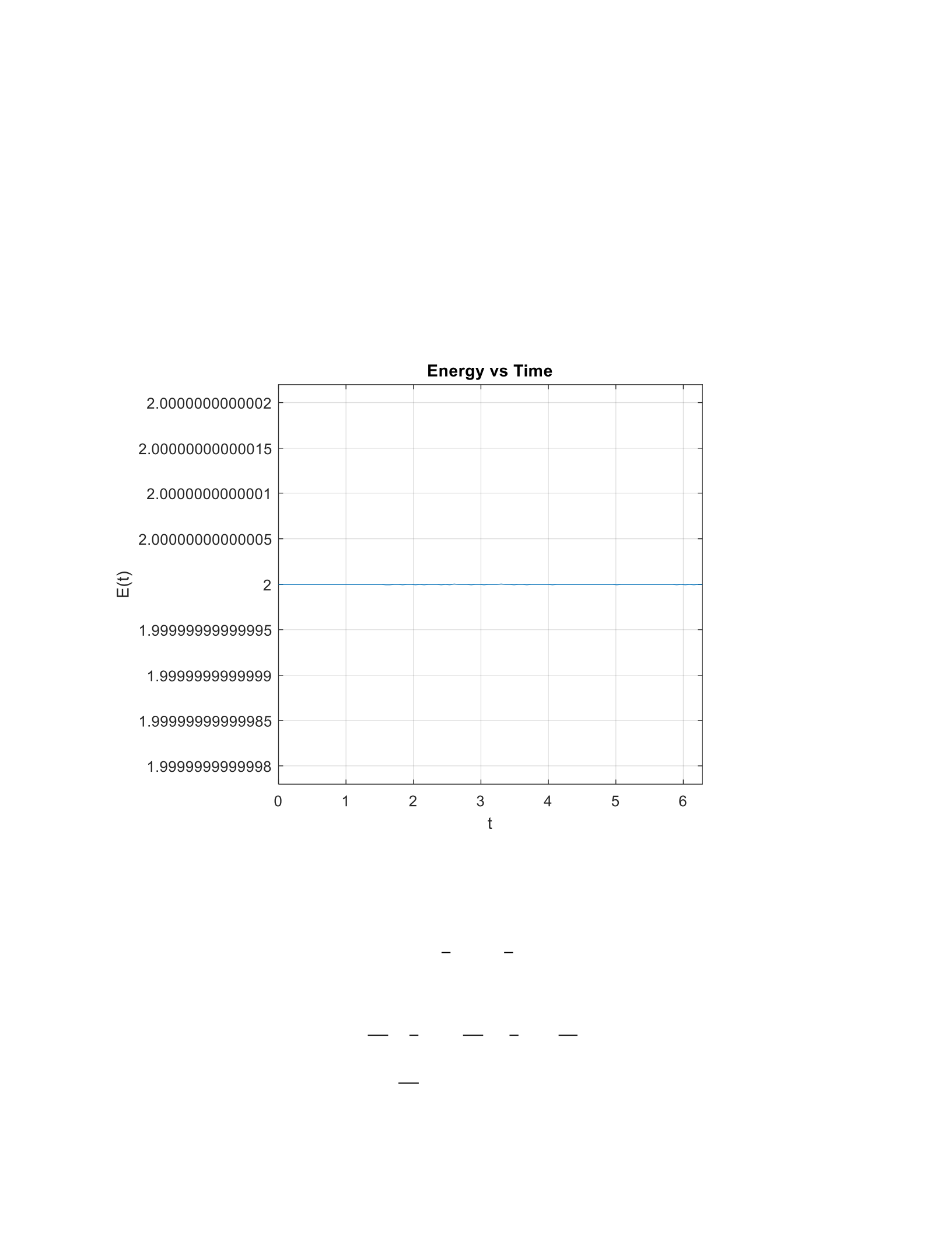
From the graph we see that energy is constant at 2.0 and independent of time (t). Since the energy
comes out to be a constant this roves that energy is conserved at all time.
B)
𝐸 = 1
2𝑚𝑣2+1
2𝑘𝑦2
Differentiate with respect to time
𝑑𝐸
𝑑𝑡 =1
2𝑚(2𝑣 𝑑𝑉
𝑑𝑡) + 1
2𝑘(2𝑣 𝑑𝑦
𝑑𝑡)
𝑑𝐸
𝑑𝑡 = 𝑣(𝑚(𝑔)+ 𝑘(𝑦))
𝑑𝐸
𝑑𝑡 = 0
Hence the energy is constant.
c)
figure
plot(y, v)
xlabel('y')
ylabel('v')
title('Phase Plot')
grid on
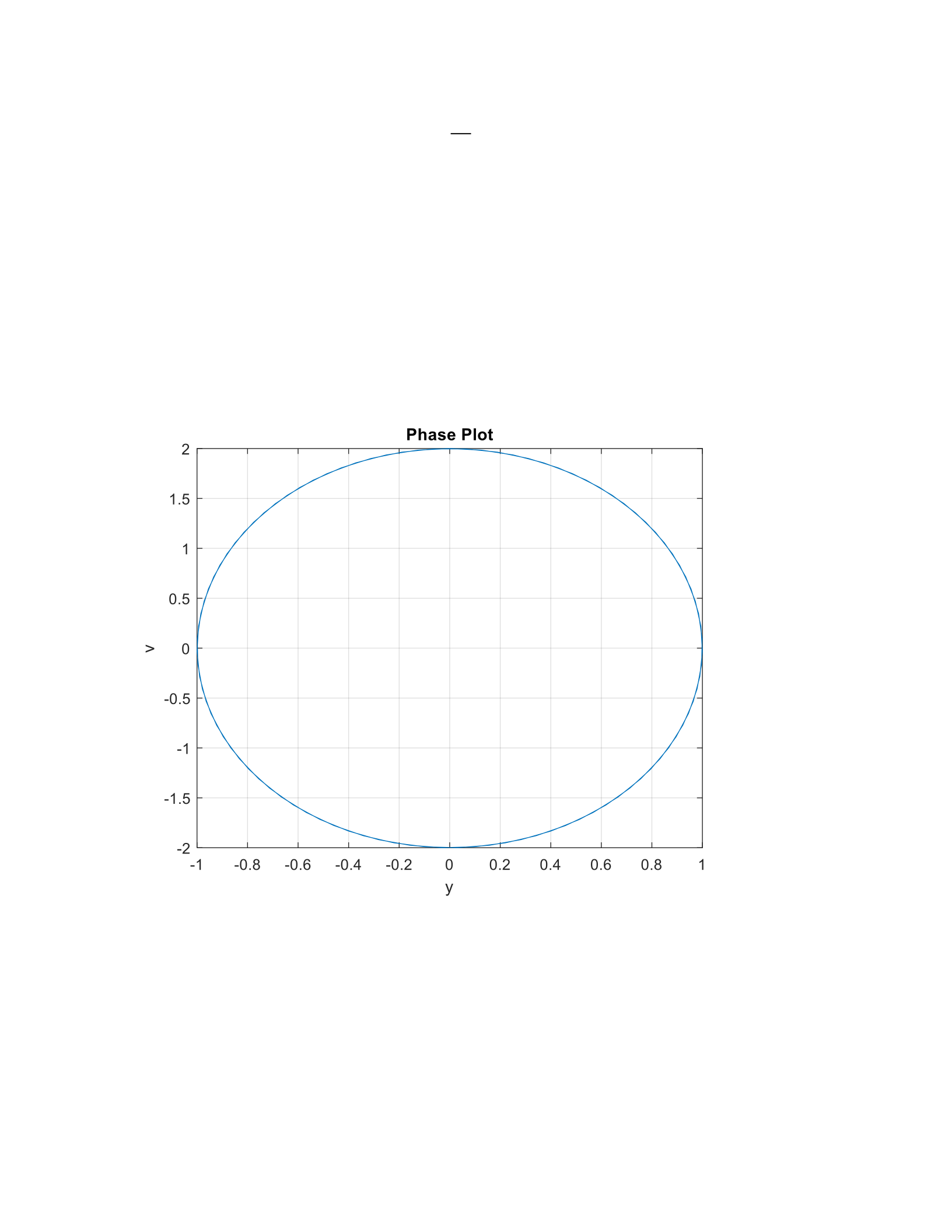
No, the curve never comes close to the origin. The curve suggest that neither value are at zero
simultaneously, or that when one value reaches its minimum the other is reaching its maximum
This confirms that velocity is zero when the displacement is maximum and when the velocity is
maximum the displacement is zero.
EX 3
A)

function LAB05ex1a
m = 1; % mass [kg]
k = 4; % spring constant [N/m]
c = 0; % friction coefficient [Ns/m]
omega0 = sqrt(k/m); p = c/(2*m); y0 = 0.1; v0 = 0; % initial
conditions
[t,Y]=ode45(@f,[0,10],[y0,v0],[],omega0,p); % solve for 0<t<10
y=Y(:,1); v=Y(:,2); % retrieve y, v from Y
figure(1); plot(t,y, 'b+-' ,t,v, 'ro-' ); % time series for y and v
figure(2); E=(.5*m*(v.^2))+(.5*k*(y.^2))
plot(t,E, 'k-' )
grid on
for i=1: length(y)
M(i)=max(abs(y(i:end )));
end
i = find(M <0.06); i = i(1)
disp([
'|y| <0.06 for t > t1 with'
num2str(t(i-1))
'< t1 <'
num2str(t(i))])
%------------------------------------------------------
function dYdt= f(t,Y,omega0,p)
y = Y(1); v= Y(2);
dYdt = [v;-2*p*v-omega0^2*y];
end
end
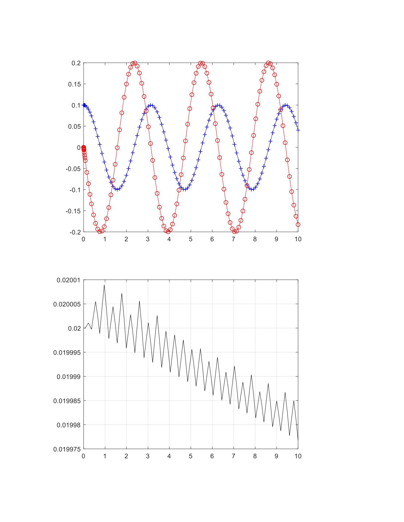
E=0.020
i = 116
B)
From the graph the maximum velocity is around 0.1995 m/s and it occurs around 2.39 s.
C)
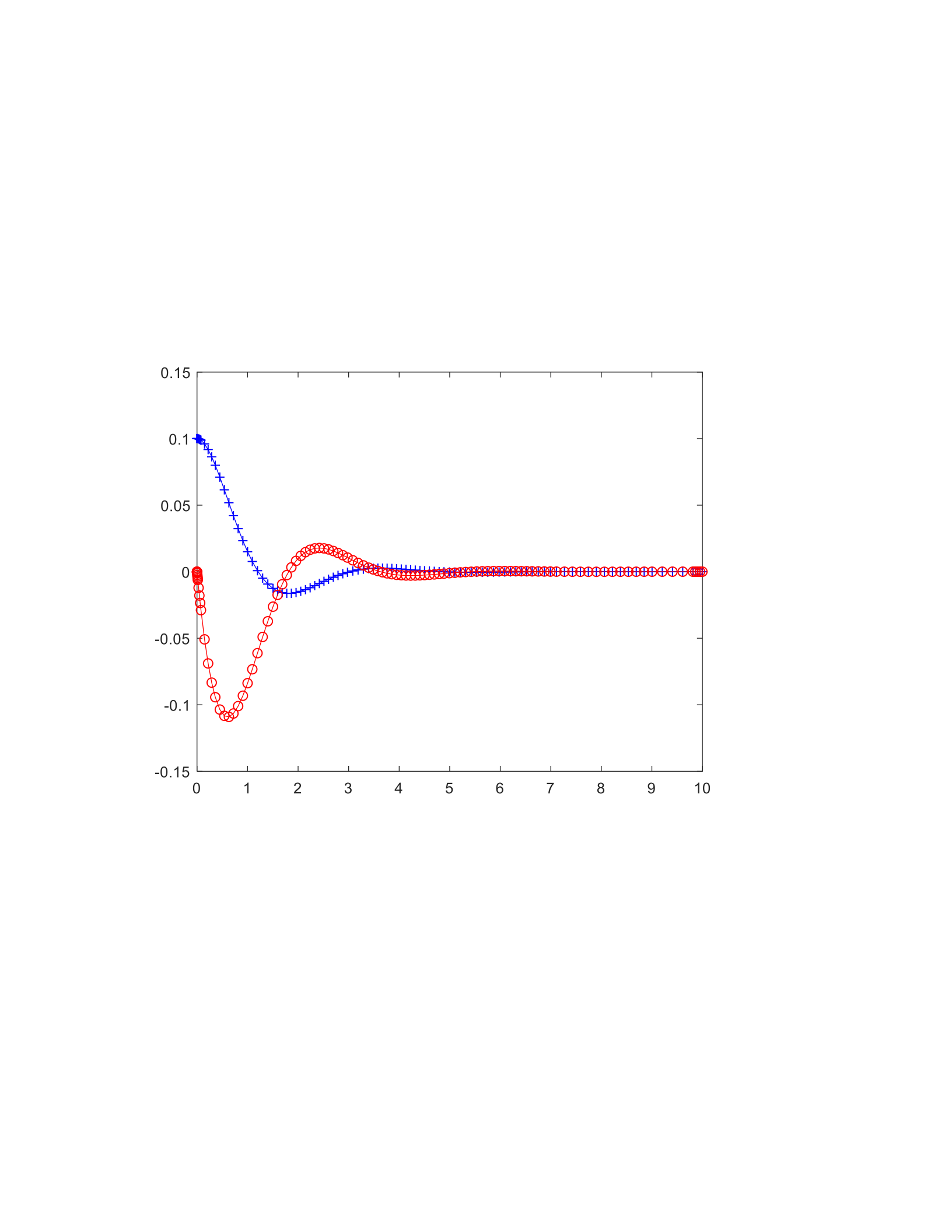
Graph 1: C=2
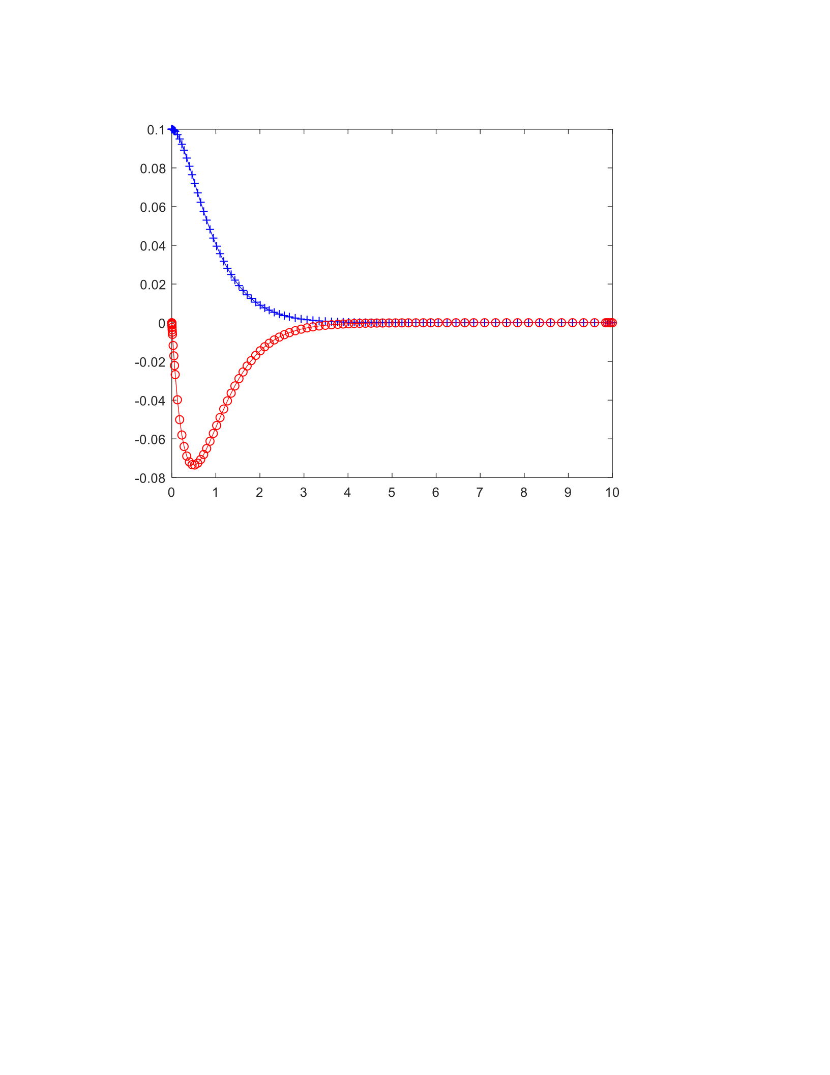
Graph 2: C=4
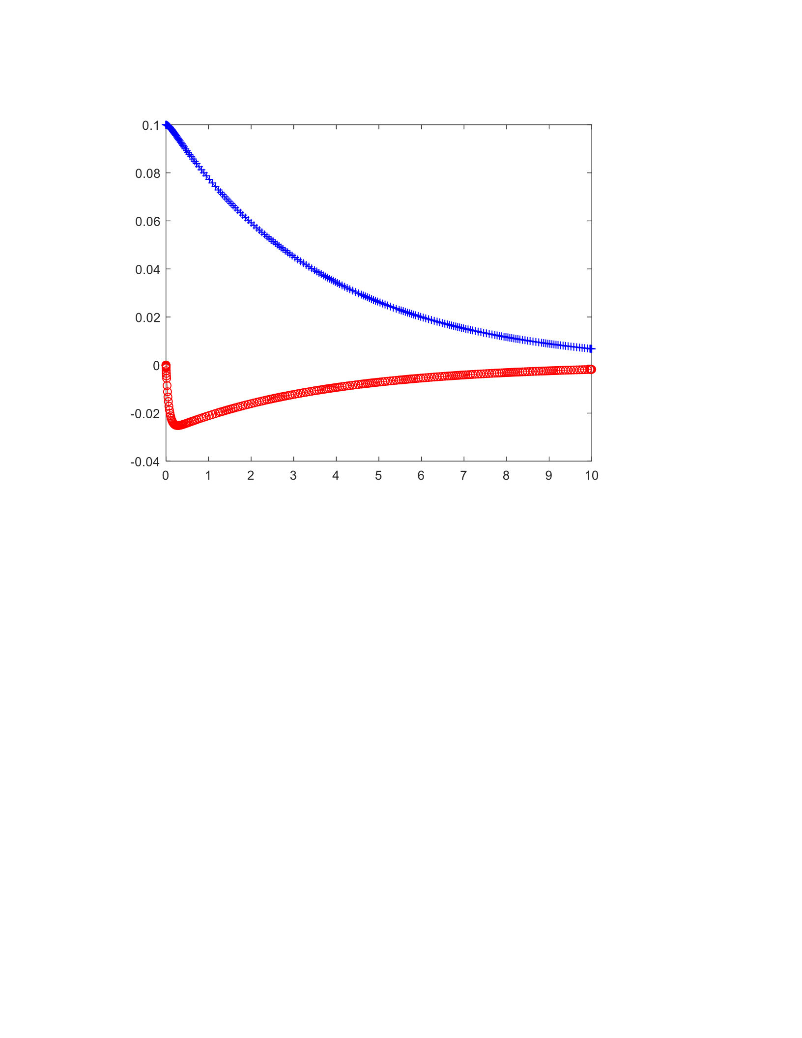
Graph 3: C=15
As the value of ‘c’ is increased the damping force increases reducing the maximum value attained
by the mass and also the mass comes to a rest slowly as ‘c’ is increased.
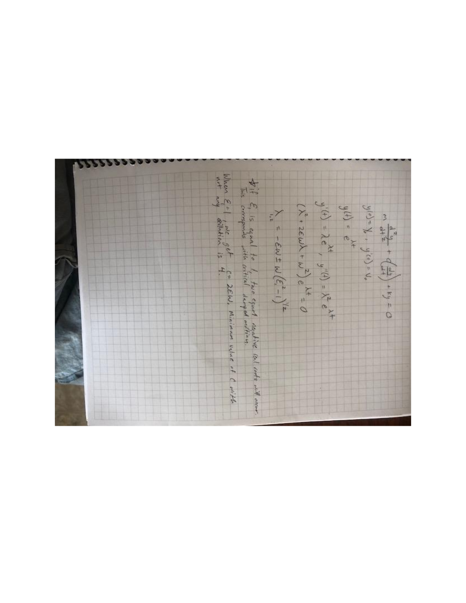
D)
EX4
A)
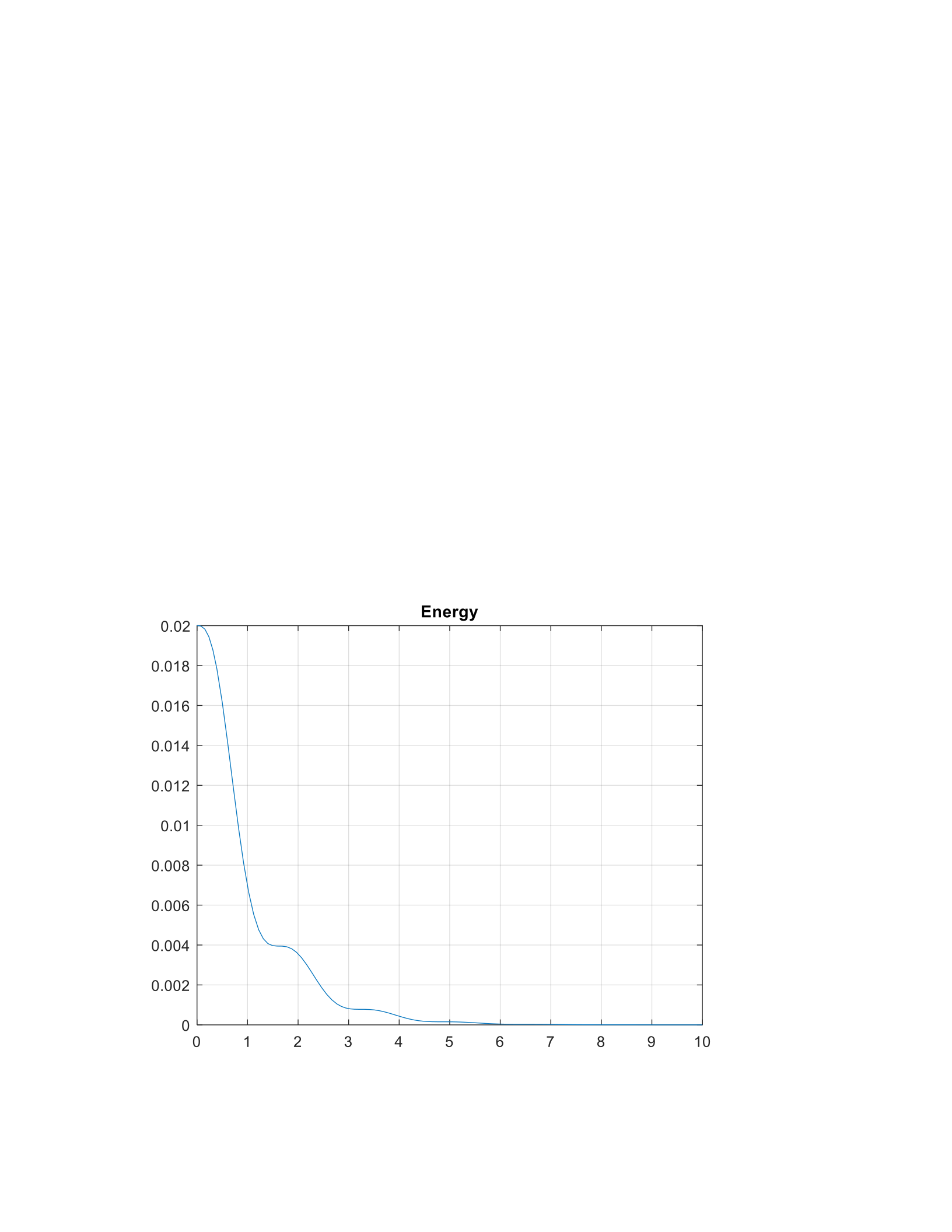
function LAB05ex1a
m = 1; % mass [kg]
k = 4; % spring constant [N/m]
c = 1; % friction coefficient [Ns/m]
omega0 = sqrt(k/m); p = c/(2*m);
y0 = 0.1; v0 = 0; % initial conditions
[t,Y]=ode45(@f,[0,10],[y0,v0],[],omega0,p); % solve for 0<t<10
y=Y(:,1); v=Y(:,2); % retrieve y, v from Y
figure(1); plot(t,y,'b+-',t,v,'ro-'); % time series for y and v
legend('y(t)','y''(t)=v(t)')
title('c=1')
figure(2)
E=.5*m*v.^2+.5*k*y.^2;
plot(t,E)
title('Energy')
grid on
%------------------------------------------------------
function dYdt= f(t,Y,omega0,p)
y = Y(1); v= Y(2);
dYdt = [v;-2*p*v-omega0^2*y];
B)
𝐸 = 1
2𝑚𝑣2+1
2𝑘𝑦2
Differentiate with respect to time
𝑑𝐸
𝑑𝑡 =1
2𝑚(2𝑣 𝑑𝑉
𝑑𝑡) + 1
2𝑘(2𝑣 𝑑𝑦
𝑑𝑡)
𝑑𝐸
𝑑𝑡 = 𝑣(𝑚(𝑔)+ 𝑘(𝑦))
𝑑𝐸
𝑑𝑡 = −𝑐𝑣
C)
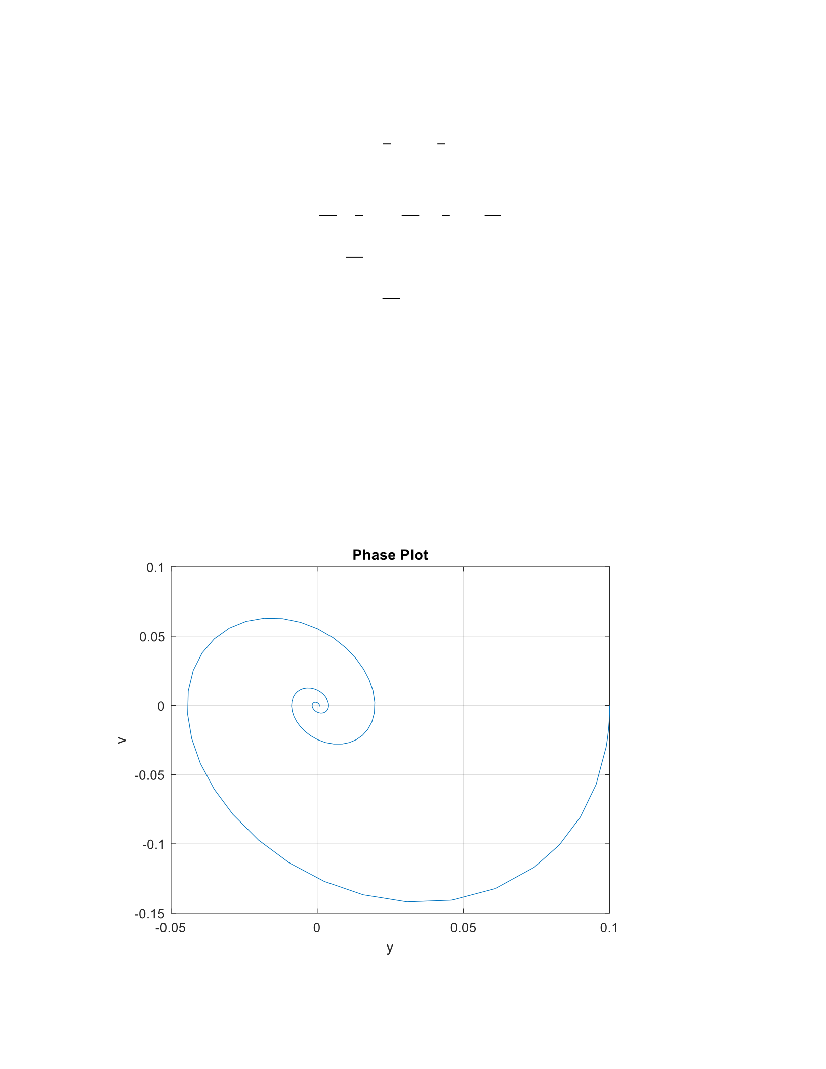
As you can see from the graph below. The time plot comes closer to its origin. This suggests that
energy is not totally conserved. Hence the entire kinetic energy of the mass is not converted into
spring potential energy and vice-versa. Due to the damping factors there is a loss of energy and
the mass doesn’t continue to oscillate and finally stops after some time.

function LAB05ex1a
m = 1; % mass [kg]
k = 4; % spring constant [N/m]
c = 1; % friction coefficient [Ns/m]
omega0 = sqrt(k/m); p = c/(2*m);
y0 = 0.1; v0 = 0; % initial conditions
[t,Y]=ode45(@f,[0,10],[y0,v0],[],omega0,p); % solve for 0<t<10
y=Y(:,1); v=Y(:,2); % retrieve y, v from Y
figure
plot(y, v)
xlabel('y')
ylabel('v')
title('Phase Plot')
grid on
%------------------------------------------------------
function dYdt= f(t,Y,omega0,p)
y = Y(1); v= Y(2);
dYdt = [v;-2*p*v-omega0^2*y];

