



Lab 3 MAT 275
Name: Morgan Johnson TA: Jorly C. Lab Time: Friday 4:30-5:20pm
Exercise 1................................................................................................................ 1
Exercise 2................................................................................................................ 2
Exercise 3................................................................................................................ 6
Exercise 4................................................................................................................ 7
Exercise 5................................................................................................................ 8
Exercise 1
Use Euler's method to solve y'= 2y with y(0)= 3 numerically
t= linspace(0, 0.5, 100);
y= 3*exp(2*t);
a) Determine the Eulers approximation for N = 500 and N = 5000
f= inline('2*y', 't', 'y'); %inline function
[t5, y5]= euler(f, [0, 0.5], 3, 5); % N=5
y5(end);
[t50, y50]= euler(f, [0, 0.5], 3, 50); % N=50
y50(end);
[t500, y500]= euler(f, [0, 0.5], 3, 500); % N=500
y500(end);
[t5000, y5000]= euler(f, [0, 0.5], 3, 5000); % N=5000
y5000(end);
% Calculate the error. Error = Exact - Approximation
e5 = y(end) - y5(end); % error at N=5
e50 = y(end) - y50(end); % error at N=50
e500 = y(end) - y500(end); % error at N=500
e5000 = y(end) - y5000(end); % error at N=5000
% Calculate the ratio of errors
ratio1= e5/e50; % ratio of error between 5 and 50
ratio2= e50/e500; % ratio of error between 5 and 50
ratio3= e500/e5000; % ratio of error between 5 and 50

% tabulate the data
N= [5;50;500;5000];
Approximation= [y5(end);y50(end);y500(end);y5000(end)];
Error= [e5;e50;e500;e5000];
Ratio= [0;ratio1;ratio2;ratio3];
T=table(N,Approximation,Error,Ratio)
T =
N Approximation Error Ratio
____ _____________ __________ ______
5 7.465 0.68989 0
50 8.0748 0.080081 8.6148
500 8.1467 0.0081399 9.8381
5000 8.154 0.00081534 9.9835
b) The ratio of error is going to 10 and the step size is decreasing by a factor of 10
each time. Every time the stepsize is decreased by a factor 10, the error is reduced
by a factor of 10.
c) The function is concave up so the tangent is below the graph thus there is an
underestimation.
Exercise 2
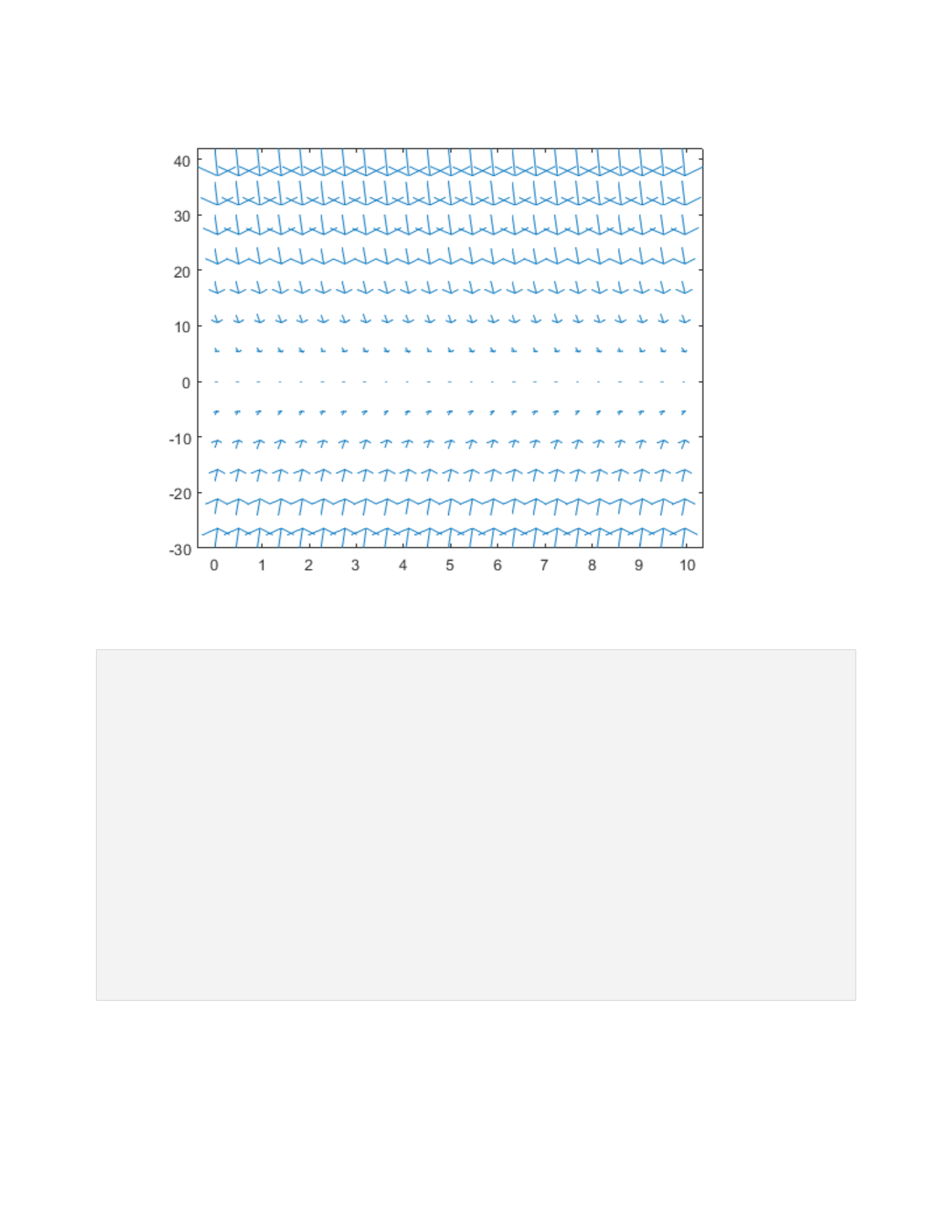
Graphing a directional field 4 graphs
a)
figure(1)
t = 0:.45:10; y = -30:6:42 ; % define grid of values in t and y direction
[T,Y]=meshgrid(t,y); % creates 2d matrices of points in the ty-plane
dT = ones(size(T)); % dt=1 for all points
dY = -2*Y; % dy = -2*y; this is the ODE
quiver(T,Y,dT,dY) % draw arrows (t,y)->(t+dt, t+dy)
axis tight % adjust look
hold on
hold of
b)
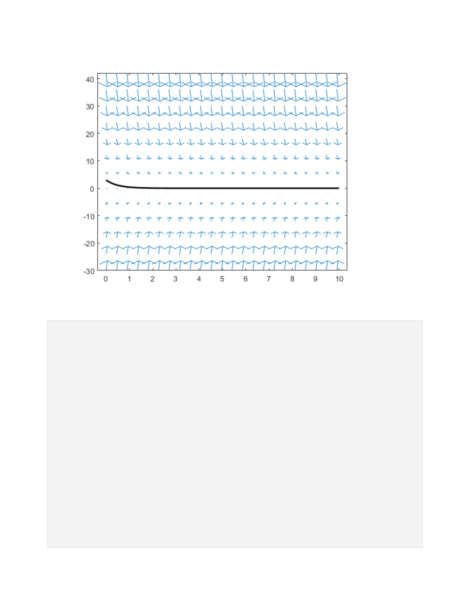
figure(2)
t = 0:.45:10; y = -30:6:42 ; % define grid of values in t and y direction
[T,Y]=meshgrid(t,y); % creates 2d matrices of points in the ty-plane
dT = ones(size(T)); % dt=1 for all points
dY = -2*Y; % dy = -2*y; this is the ODE
quiver(T,Y,dT,dY) % draw arrows (t,y)->(t+dt, t+dy)
axis tight % adjust look
hold on
% Exact solution
t = linspace(0,10,200);
y = 3*exp(-2*t);
plot(t,y,'k-', 'linewidth',2)
hold of
c)
figure(3)
t = 0:.45:10; y = -30:6:42 ; % define grid of values in t and y direction
[T,Y]=meshgrid(t,y); % creates 2d matrices of points in the ty-plane
dT = ones(size(T)); % dt=1 for all points
dY = -2*Y; % dy = -2*y; this is the ODE
quiver(T,Y,dT,dY) % draw arrows (t,y)->(t+dt, t+dy)
axis tight % adjust look
hold on
% Exact solution
t = linspace(0,10,200);
y = 3*exp(-2*t);
plot(t,y,'k-', 'linewidth',2)
% Euler's Approximation for N=8
f= inline('-2*y', 't', 'y'); %inline function
[t8, y8]= euler(f, [0, 10], 3, 8); % N=8
plot(t8,y8,'ro-', 'linewidth',2)
hold of
axis([0 10 -30 40])
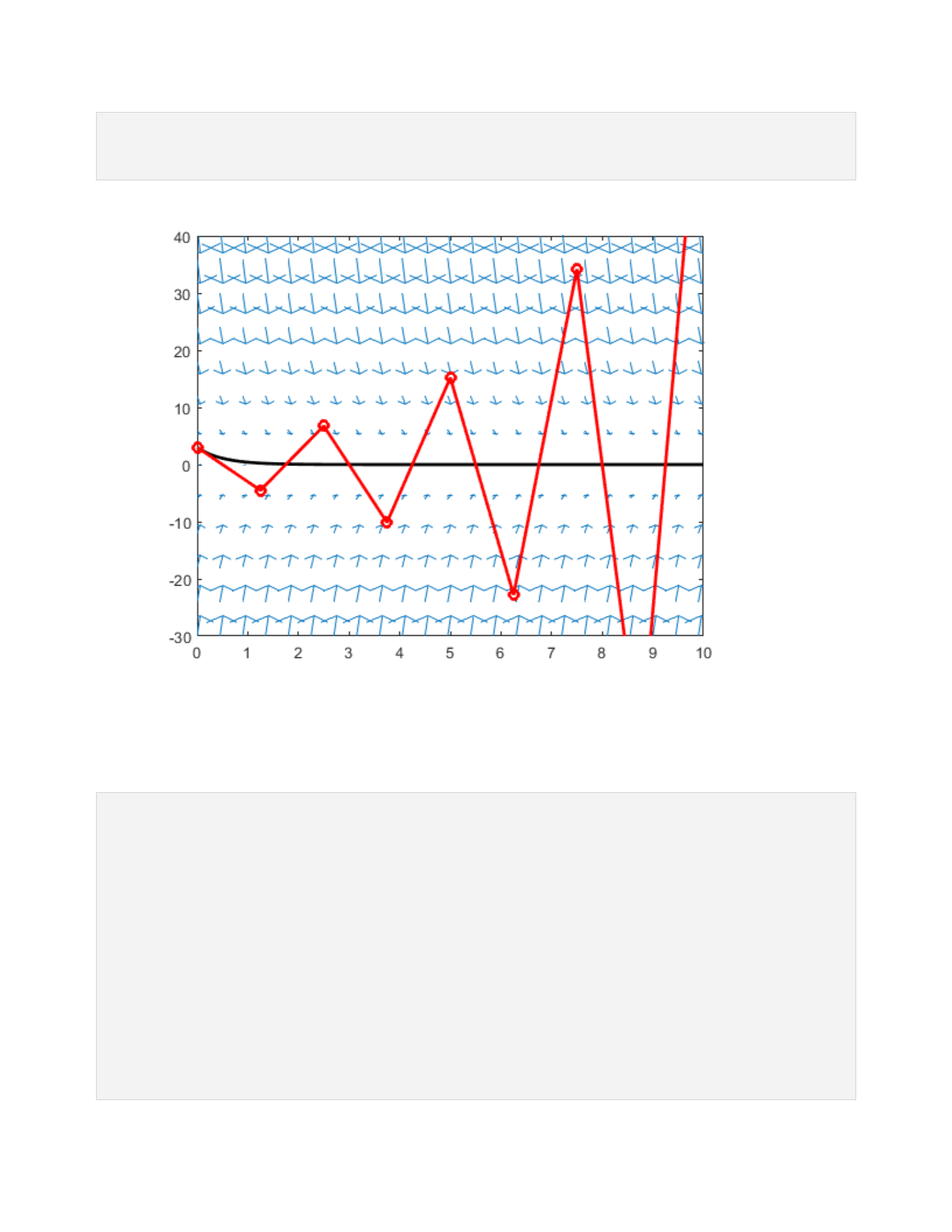
The geometry of the approximation graph indicates that the stepsize is too small
because the line follows the direction field vectors for too long.
d)
figure(4)
t = 0:.4:10; y = -1:0.4:3; % define grid of values in t and y direction
[T,Y]=meshgrid(t,y); % creates 2d matrices of points in the ty-plane
dT = ones(size(T)); % dt=1 for all points
dY = -2*Y; % dy = -2*y; this is the ODE
quiver(T,Y,dT,dY) % draw arrows (t,y)->(t+dt, t+dy)
axis tight % adjust look
hold on
% Exact solution
t = linspace(0,10,200);
y = 3*exp(-2*t);
plot(t,y,'k-','linewidth',2)
% Euler's Approximation for N=16
f= inline('-2*y', 't', 'y'); %inline function
[t16, y16]= euler(f, [0, 10], 3, 16); % N=16
plot(t16,y16,'ro-','linewidth',2)
hold of
axis([0 10 -1 3])
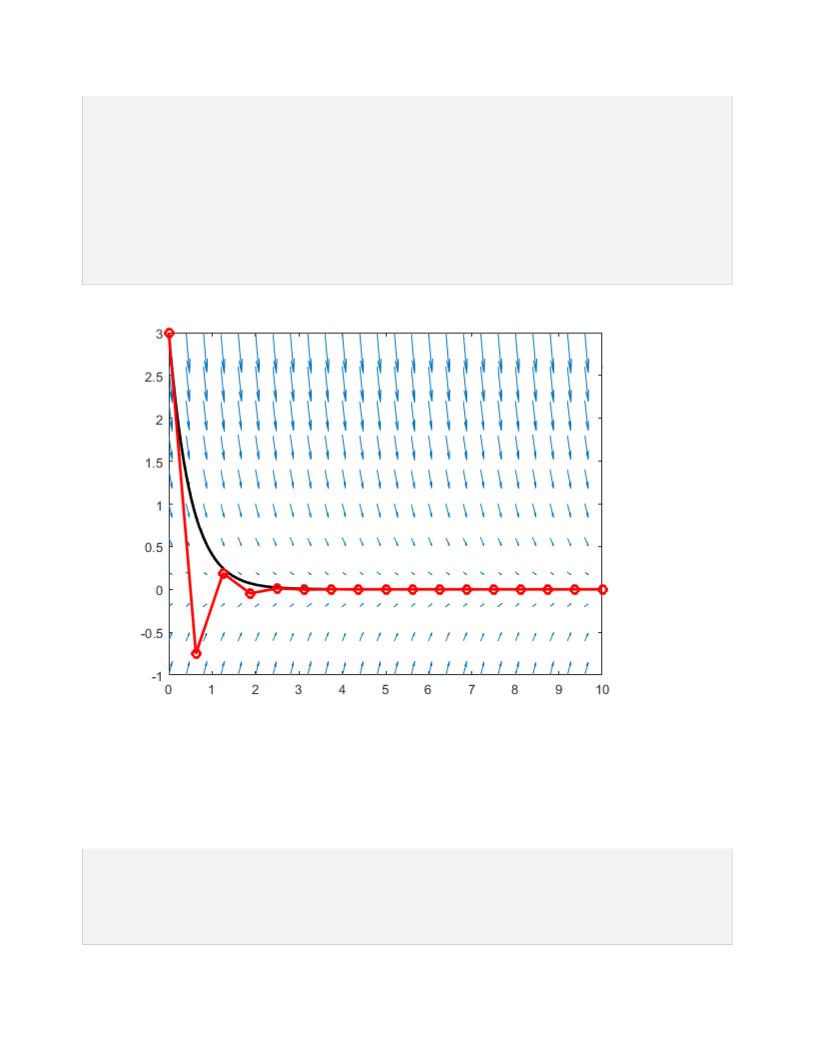
The geometry of the approximation graph indicates that the stepsize is larger but
the the line still follows the direction field vectors for too long (however not as long
as with a stepsize of 8) causing the slight oscillation at the beginning.
Exercise 3
Modify the M-file euler.m to implement the algorithm for Improved Euler
% Display contents of impeuler M-file.
type 'impeuler.m'
% Define ODE function for dy/dt = f(t,y) = 2y.

f= inline('2*y', 't', 'y');
% Compute numerical solution to IVP with 5 timesteps using "improved Euler."
[t5, y5] = impeuler(f, [0 0.5],3,5)
function [t,y] = impeuler(f,tspan,y0,N)
% Solves the IVP y' = f(t,y), y(t0) = y0 in the time interval tspan = [t0,tf]
% using Euler's method with N time steps.
% Input:
% f = name of inline function or function M-file that evaluates the ODE
% (if not an inline function, use: euler(@f,tspan,y0,N))
% For a system, the f must be given as column vector.
% tspan = [t0, tf] where t0 = initial time value and tf = final time value
% y0 = initial value of the dependent variable. If solving a system,
% initial conditions must be given as a vector.
% N = number of steps used.
% Output:
% t = vector of time values where the solution was computed
% y = vector of computed solution values.
m = length(y0);
t0 = tspan(1);
tf = tspan(2);
h = (tf-t0)/N; % evaluate the time step size
t = linspace(t0,tf,N+1); % create the vector of t values
y = zeros(m,N+1); % allocate memory for the output y
y(:,1) = y0'; % set initial condition
for n=1:N
f1= f(t(n), y(:,n));
f2= f(t(n+1), y(:,n)+h*f1);
y(:,n+1)= y(:,n) +h*(f1+f2)/2;
end
t = t'; y = y'; % change t and y from row to column vectors
end
t5 =
0
0.1000
0.2000
0.3000
0.4000
0.5000

y5 =
3.0000
3.6600
4.4652
5.4475
6.6460
8.1081
Exercise 4
Repeat all the steps from Exercise 1, except using "improved Euler"
%Use Euler's method to solve y'= 2y with y(0)= 3 numerically
t= linspace(0, 0.5, 100);
y= 3*exp(2*t);
a) Determine the Euler’s approximation for N = 500 and N = 5000 using improved
Euler
f= inline('2*y', 't', 'y'); %inline function
[t5, y5]= impeuler(f, [0, 0.5], 3, 5); % N=5
y5(end);
[t50, y50]= impeuler(f, [0, 0.5], 3, 50); % N=50
y50(end);
[t500, y500]= impeuler(f, [0, 0.5], 3, 500); % N=500
y500(end);
[t5000, y5000]= impeuler(f, [0, 0.5], 3, 5000); % N=5000
y5000(end);
% Calculate the error. Error = Exact - Approximation
e5 = y(end) - y5(end); % error at N=5
e50 = y(end) - y50(end); % error at N=50
e500 = y(end) - y500(end); % error at N=500
e5000 = y(end) - y5000(end); % error at N=5000
% Calculate the ratio of errors
ratio1= e5/e50; % ratio of error between 5 and 50

ratio2= e50/e500; % ratio of error between 5 and 50
ratio3= e500/e5000; % ratio of error between 5 and 50
% tabulate the data
N= [5;50;500;5000];
Approximation= [y5(end);y50(end);y500(end);y5000(end)];
Error= [e5;e50;e500;e5000];
Ratio= [0;ratio1;ratio2;ratio3];
T=table(N,Approximation,Error,Ratio)
T =
N Approximation Error Ratio
____ _____________ __________ ______
5 8.1081 0.046721 0
50 8.1543 0.00053555 87.239
500 8.1548 5.4284e-06 98.657
5000 8.1548 5.4357e-08 99.865
b) The ratio of error is going to 100 and the step size is decreasing by a factor of 10
each time. Every time the stepsize is decreased by a factor 10, the error is reduced
by a factor of 102 when improved Euler’s method it used.
Exercise 5
Repeat all the steps from exercise 2, except using improved Euler
% a) and b) are the same as in Exercise 2
c)
figure(5)
t = 0:.45:10; y = -30:6:42 ; % define grid of values in t and y direction
[T,Y]=meshgrid(t,y); % creates 2d matrices of points in the ty-plane
dT = ones(size(T)); % dt=1 for all points
dY = -2*Y; % dy = -2*y; this is the ODE
quiver(T,Y,dT,dY) % draw arrows (t,y)->(t+dt, t+dy)
axis tight % adjust look
hold on
% Exact solution
t = linspace(0,10,200);
y = 3*exp(-2*t);
plot(t,y,'k-', 'linewidth',2)
% Improved Euler's Approximation for N=8
f= inline('-2*y', 't', 'y'); %inline function
[t8, y8]= impeuler(f, [0, 10], 3, 8); % N=8
plot(t8,y8,'ro-', 'linewidth',2)
hold of
axis([0 10 -30 40])
d)
figure(6)
t = 0:.4:10; y = -1:0.4:3; % define grid of values in t and y direction
[T,Y]=meshgrid(t,y); % creates 2d matrices of points in the ty-plane
dT = ones(size(T)); % dt=1 for all points
dY = -2*Y; % dy = -2*y; this is the ODE
quiver(T,Y,dT,dY) % draw arrows (t,y)->(t+dt, t+dy)
axis tight % adjust look
hold on
% Exact solution
t = linspace(0,10,200);
y = 3*exp(-2*t);
plot(t,y,'k-','linewidth',2)
% Improved Euler's Approximation for N=16
f= inline('-2*y', 't', 'y'); %inline function
[t16, y16]= impeuler(f, [0, 10], 3, 16); % N=16
plot(t16,y16,'ro-','linewidth',2)
hold of
axis([0 10 -1 3])
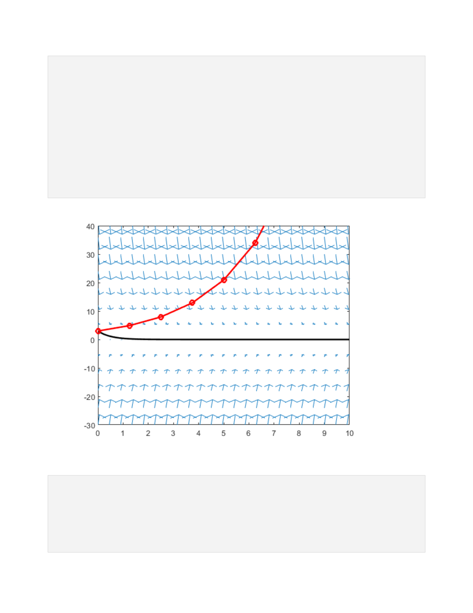
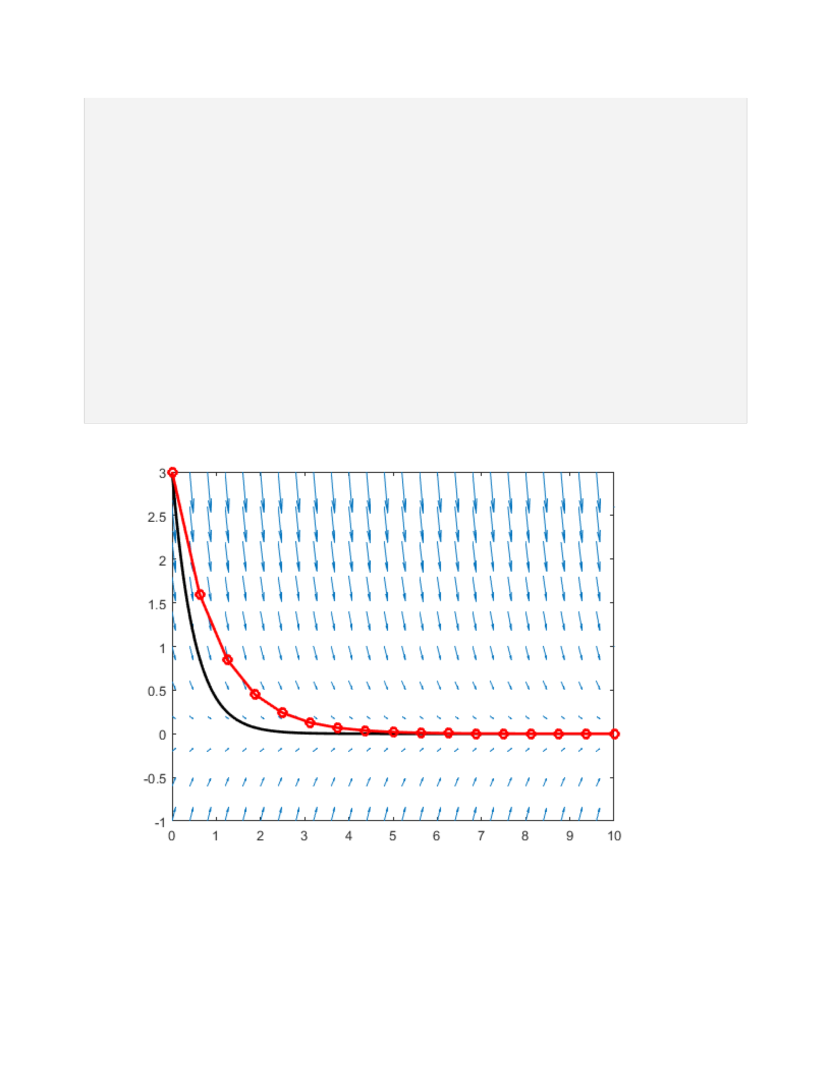
Compared to the results from using Euler’s method, the N=8 approximation is still
of but the N= 16 approximation is more accurate. The graphs of the
approximations using improved Euler’s method are smother.

