


8 2
Ey
SOR
REE
my
ew
,
AM
Xs
Awe
YS
£
keeg,
S\Fs
SS
8
x
og
4
tdi
s
2
we
RSE
SRY
oT §
Seat
Anas
rmYasy
se
See
S
ee
&
S
na
o
a
ss
k=
YAESISS
Broa
RS
FE
=
xer*cos
(theta):
yer*sin(theta};
6.
8a8e
6,
8688
&.
8886
6,
8608
6.
8886
6,
6008
&
.
B88
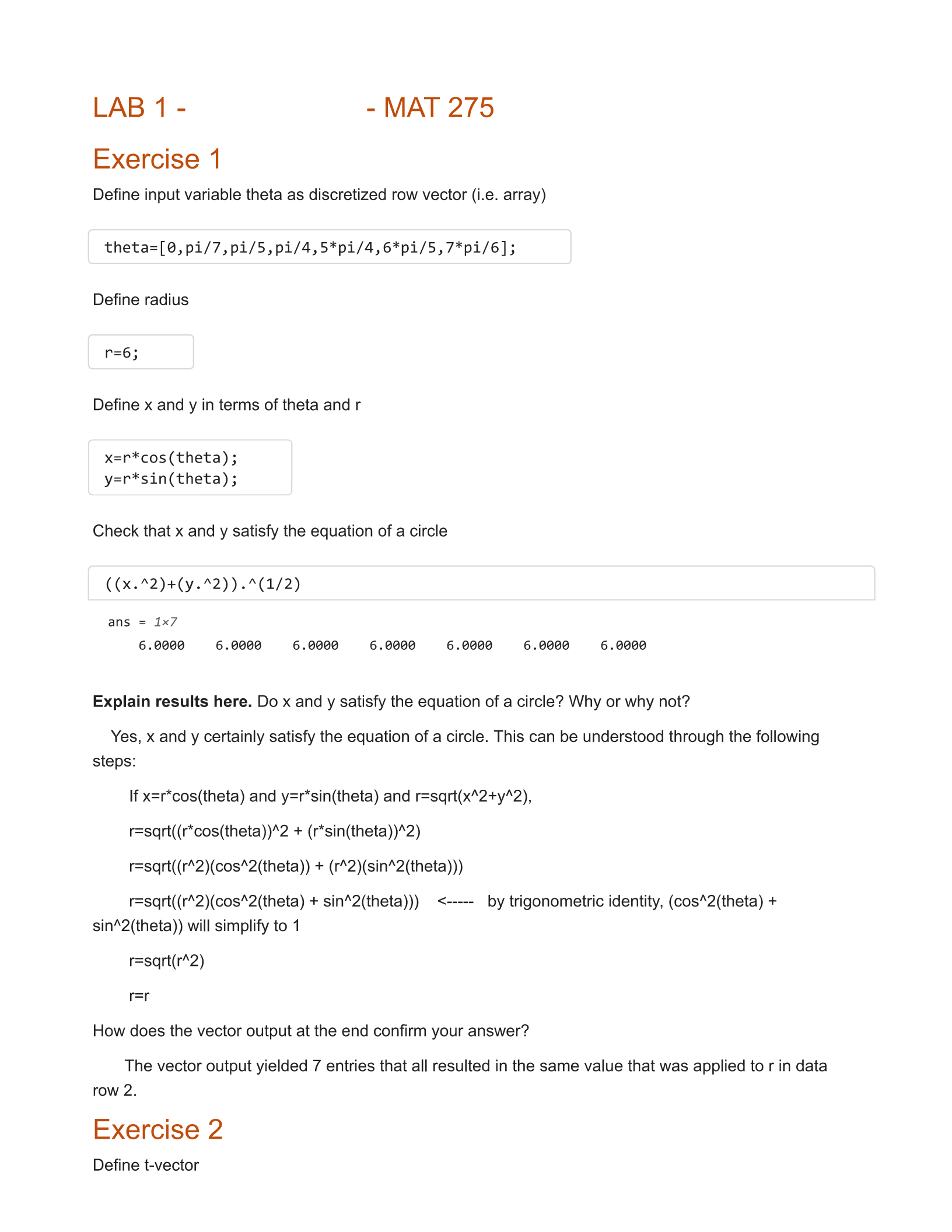
Explain
results
here.
Do
x
and
y
satisfy
the
equation
of
a
circle?
Why
or
why
not?
Yes,
x
and
y
certainly
satisfy
the
equation
of
a
circle.
This
can
be
understood
through
the
following
steps:
if
x=r*cas(thela)
and
y=rsin(theta)
and
r=sario“2+y*2),
r=sort((r*cos(theta}}*2
+
(r*sin(theta))*2)
r=sqri((r’2
icos*2(theta))
+
(*2\sin*2ttheta))
r=sqri((r’2
icos*2(theta)
+
sin2itheta}}}
<----
by
trigonometric
identity,
(cos*2(theta})
+
sin’2(theia})
will
simplify
to
7
resqrt(r’2)}
rar
How
does
the
vector
output
at
the
end
confirm
your
answer?
The
vector
output
yielded
7
entries
that
all
resulted
in
the
sare
value
that
was
applied
to
rin
data
row
2.
Detine
t-vector
t=4:0.2:20;
t
=
1x81
4.8000 4.2000 4.4000 4.6000 4.8000
5.0000
Define
y-vector
y=((exp(t./10)).*cos(t.*2))./((6.3*t.%3)+5);5
y
=
1x81
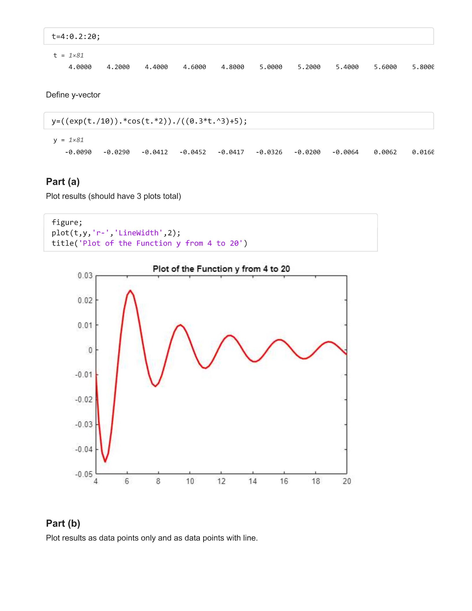
Part
(a)
Plot
results
(should
have
3
plots
total)
figure;
plot(t,y,'r-',
'LineWidth',2);
title('Plot
of
the
Function
y
from
4 to
20')
0.03
7
Plot
of
the
Function
y
from
4
to
20
5.2000
-8.0200
5.4000
-0.0064
-0.071}
-0.02
-0.03
-0).04
-
0.05
' ! ! !
!
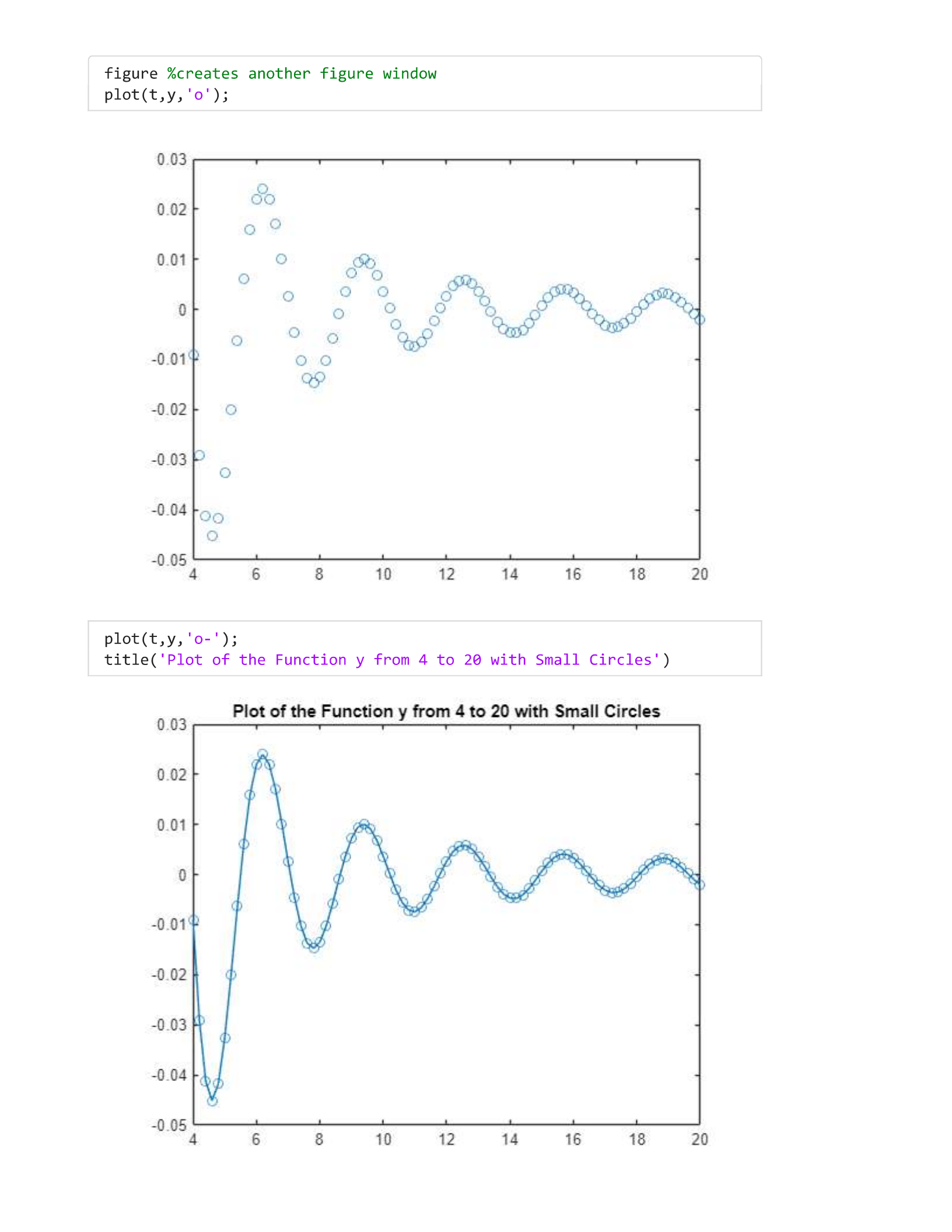
Part
(b)
Plot results
as
data
points
only
and
as
data
points
with
line.
20)
5.6000
6.0062
5.
800€
6.016€
figure
%creates
another
figure
window
plot(t,y,‘'0');
0)
03
T
T
T 1 T
T
T
‘
oo2t
oo
]
O
i)
0.01+
o
ore
J
o
MO.
3
:
OF
2
.
ci
Re
,.
on
ce
0
mo
oO
,
oO
“ags
}-
4,
iE
=“
Os?
re
Cl
(J
0.01%
Oo
J
Oy
0.02+
oO
4
O03F
_
-
Ly
-0.04
Fo,
4
-0
045
i
i
i i i i i
4 6 8 10 12
14
16
12 20
plot(t,y,'o-');
title('Plot
of
the
Function
y
from
4 to
20
with
Small
Circles’)
Plot
of
the
Function
y
from
4 to
20
with
Small
Circles
0.03
0.02+
%
1
I \
0.01F
hi
Api
|
i
a.
ei:
ri
hi
7
"]
ie
:
a
*
iy
oF
i
i
\
LE
&
i
Se.
J
H
a
‘be
i
vk
Ro
a
a
-0.01%
,
¢
|
so!
0.02
qi
4
-0.03
#
1
a
-0.04
Fy
4,
4
Ao
-f)
645
i
i
i i i i i
4 6 8 10 12
14
16
18 20

Exercise
3
Create
t-vector
(choose
enough
elements
so
that
plot
is
smooth!)
ct
ll
0:0.01:5;
ct
ll
1x501
0
8.0100
6.8200
@.0300 @.0400
Define
x,
y,
x
components
in
terms
of
t
@.0500 @.0600 @.8700
x
=
7*cos(8.*t);
y
=
7*sin(8.*t);
z
=
6.*t;
Plot results
figure;
plot3(x,y,Z);
grid
on
30
~
254
20
4
15
~
10
~
5
-10
-410
Exercise
4
Define
input
variable
as
vector
6.8800
@.898€
x=
linspace(-pi/2,pi/2,10@);
Define
y
and
z
y
=
sin(2.*x);
Z =
2.*x-(4/3).*x.43;
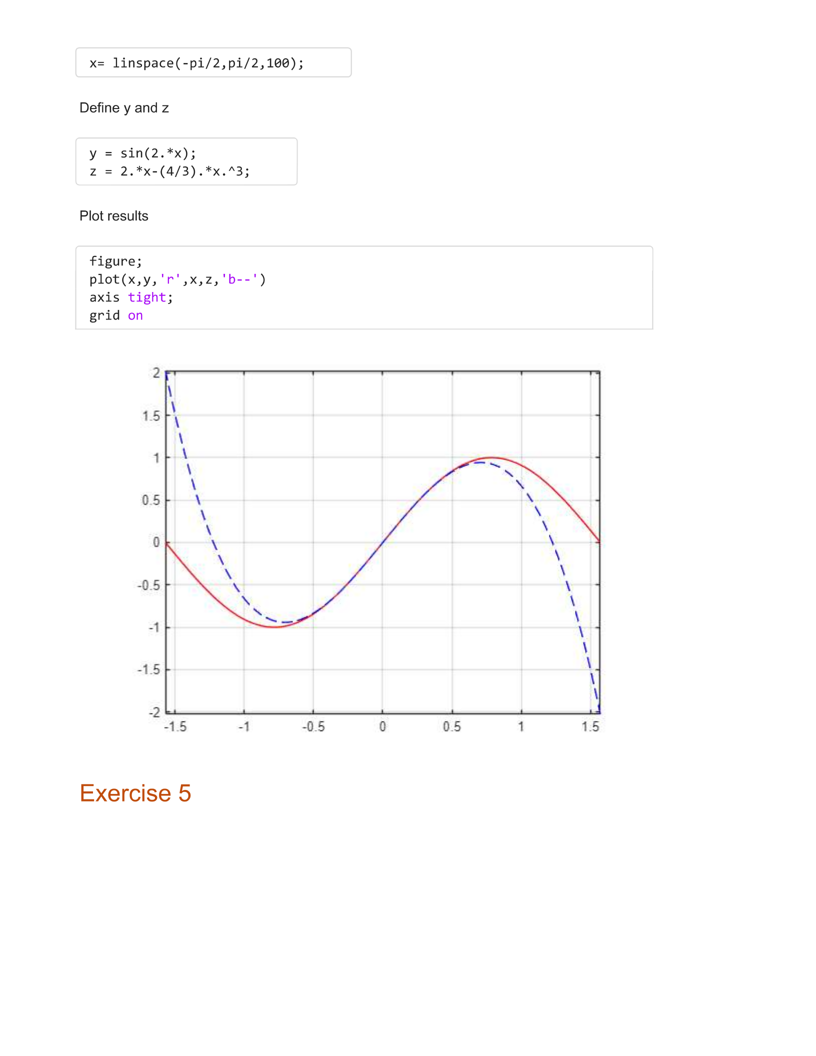
Plot
results
figure;
plot(x,y,
"re"
,X,Z;
‘b--')
axis tight;
grid
on
Exercise
5
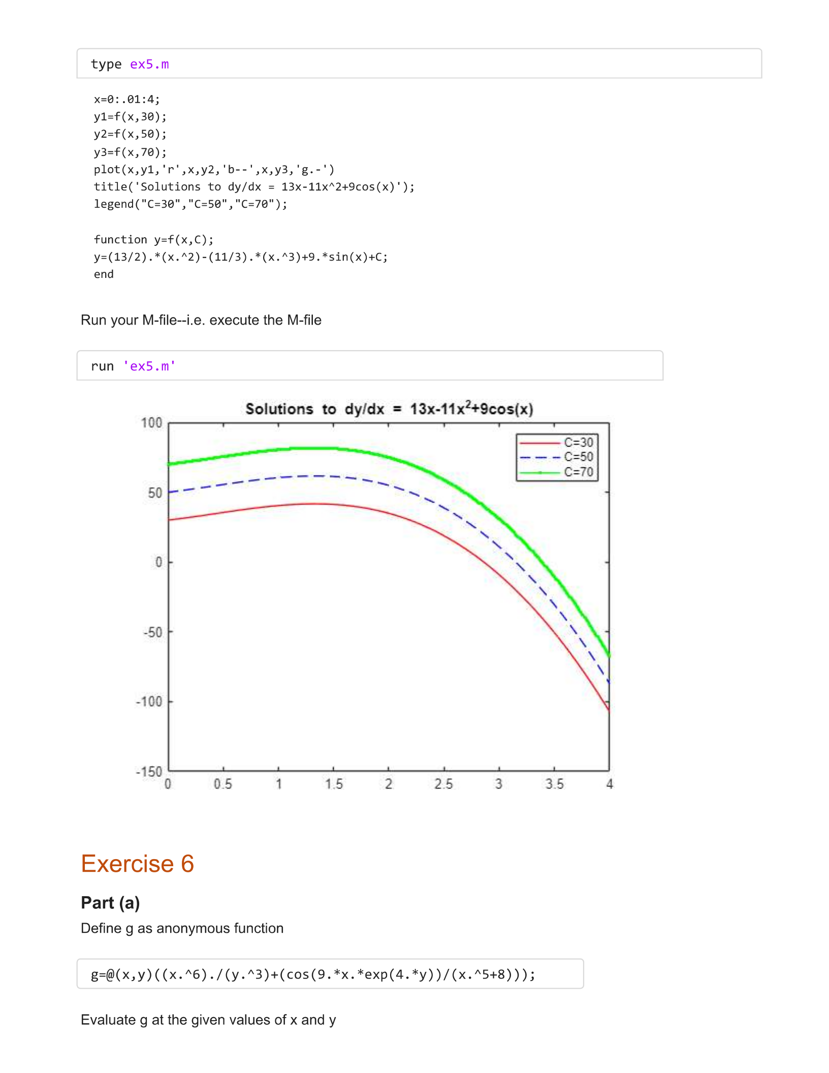
type
ex5.m
x=0:
.01:4;
y1=f
(x,
30);
y2=F
(x,
50);
y3=f
(x,
7@);
plot(x,y1,
'r',x,y2,'b--',x,y3,
'g.-")
title('Solutions
to
dy/dx
=
13x-11x*2+9cos(x)');
legend("C=30",
"C=50",
"C=70");
function
y=f(x,C);
y=(13/2).*(«.%2)-
(11/3)
.*(x.4%3)+9.*sin(x)+C;
end
Run
your
M-file--i.e.
execute
the
M-file
run
‘ex5.m'
Solutions
to
dy/dx
=
13x-11x*+9cos(x)
100
'
7
!
q
1
'
C=30
a
sew
O=50
C=/0
0
0.5
1
ES
2
25
3
Exercise
6
Part
(a)
Define
g
as
anonymous
function
g=@(x,y)((x.%6)./(y.%3)+(cos(9.*x.
*exp(4.
*y)
)/(x.%5+8)));
Evaluate
g
at
the
given
values
of
x
and
y
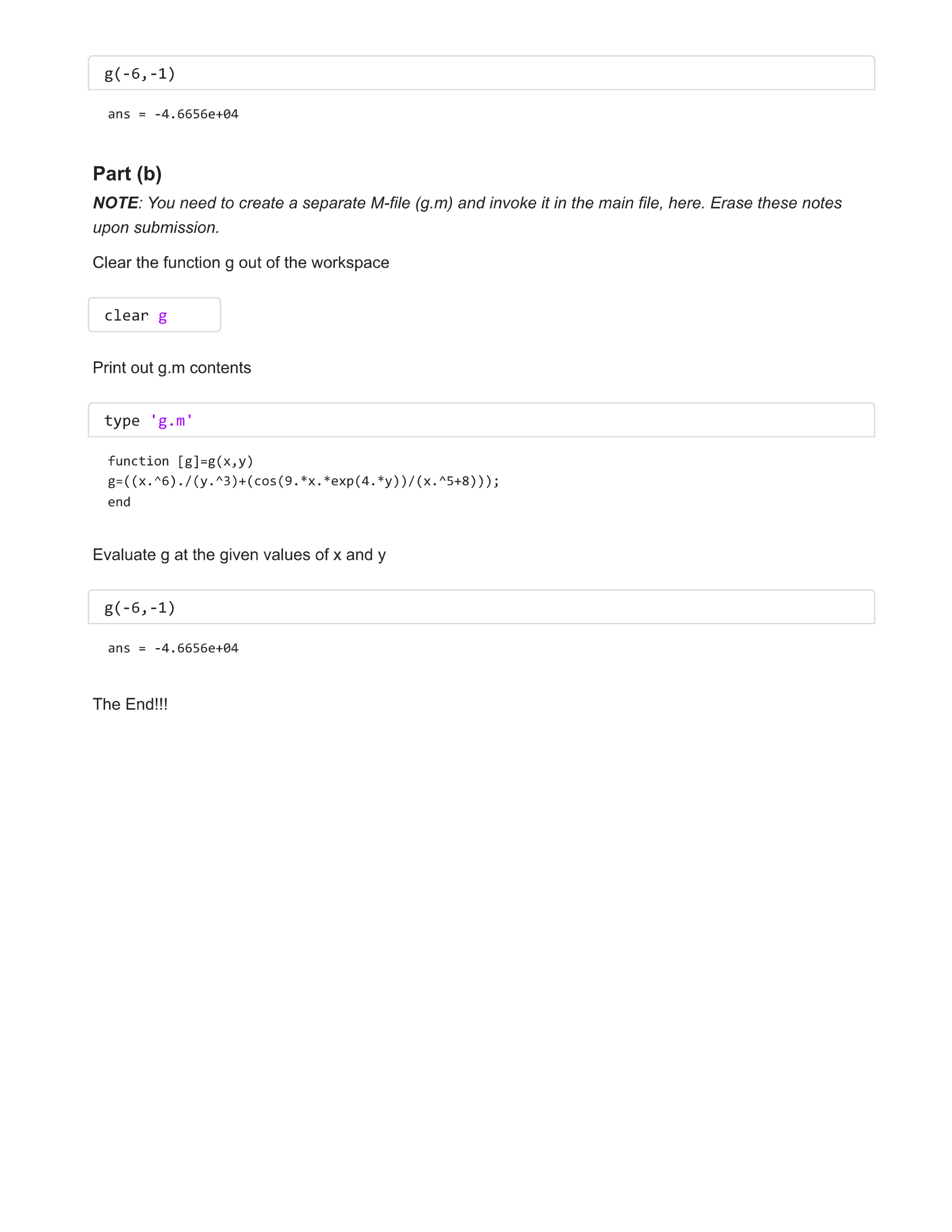
Part
(b)
NOTE:
You
need
to
creaie
a
separate
M-file
(g.m)
and
invoke
it
in
the
main
file,
here.
Erase
these
notes
UDON
SUBMISSION.
Ciear
the
function
g
out
of
the
workspace
function
[gl=e(x,y)
e=((x.%6)./Cy.*3)4(c0s
(9.
*x.
"exp
(4,
Fy3
9
/
0x.
%548)
553
end
Evaluate
g
at
the
given
values
of
x
and
y
The
Endl!

