


Mat 275
Lab 04 MATLAB solvers for first order IVPs
Jianyang Hu
%Exercise 1
%Part a
function LAB4ex1
format long
tf=40;
t0=0;
Y0=[-1;0];
[t,Y]=ode45(@f,[t0,tf],Y0);
y=Y(:,1);
v=Y(:,2);
figure(1);
grid on;
plot(t,y,'b-+',t,v,'ro-')
legend('y(t)','v(t)=y''(t)')
grid on;
ylim([-1.5,1.5]);
[t,Y(:,1)]
figure(2);
plot(y,v)
axis square;
xlabel('y'); ylabel('v=y''(t)');
grid on
ylim([-1.5,1.5]);
xlim([-1,1]);
end
function dYdt=f(t,Y)
y=Y(1);
v=Y(2);
dYdt=[v;cos(t)-4*v-3*y];
end

%Part b
The approximate t values for which y has a local max or min
%Part c
The max and the min of y is .2235 and -.2235.
It behave sine wave in long term.
%Part d
function LAB4ex1A
t0=0;
tf=40;
Y0=[1.5;5];
[t,Y]=ode45(@f,[t0,tf],Y0);
y=Y(:,1);
v=Y(:,2);
figure(1);
plot(t,y,'b-+',t,v,'ro-')
legend('y(t)','v(t)=y''(t)')
grid on;
ylim([-1.5,1.5]);
[t,Y(:,1)]
figure(2);
plot(y,v)
axiss quare;
xlabel('y'); ylabel('v');
grid on
ylim([-1.5,1.5]); xlim([-1,1]);
t
y
Local min or max
2.134
-.0903
max
4.128
-.2503
min
7.646
.2155
max
10.552
-.2233
min
13.663
.2236
max
16.785
-.2234
min
19.932
.2235
max
23.073
-.2235
min
26.215
.2235
max
29.357
-.2235
min
32.498
.2235
max
35.639
-.2235
min
38.781
.2235
max

end
function dYdt=f(t,Y)
y=Y(1);
v=Y(2);
dYdt=[v; cos(t)-4*v-3*y];
end
The modified graph of y(t) appears to have the same long term behavior as the graph of y(t). This is
because the only difference between the two graphs is the initial conditions. The functions were exactly the
same.
%Exercise 2
%Part a
function LAB4ex2B
t0=0;
tf=40;
Y0=[-1;0];
[t,Y]=ode45(@f,[t0,tf],Y0);
y=Y(:,1);
v=Y(:,2);
[te,Ye]=euler(@f,[0,40],Y0,400);
figure(1);
plot(t,y,'b',t,v,'r')
legend('y(t)','v(t)=y''(t)')
grid on;
figure(2);
plot(y,v,'k')
axis square;
xlabel('y'); ylabel('v');
grid on
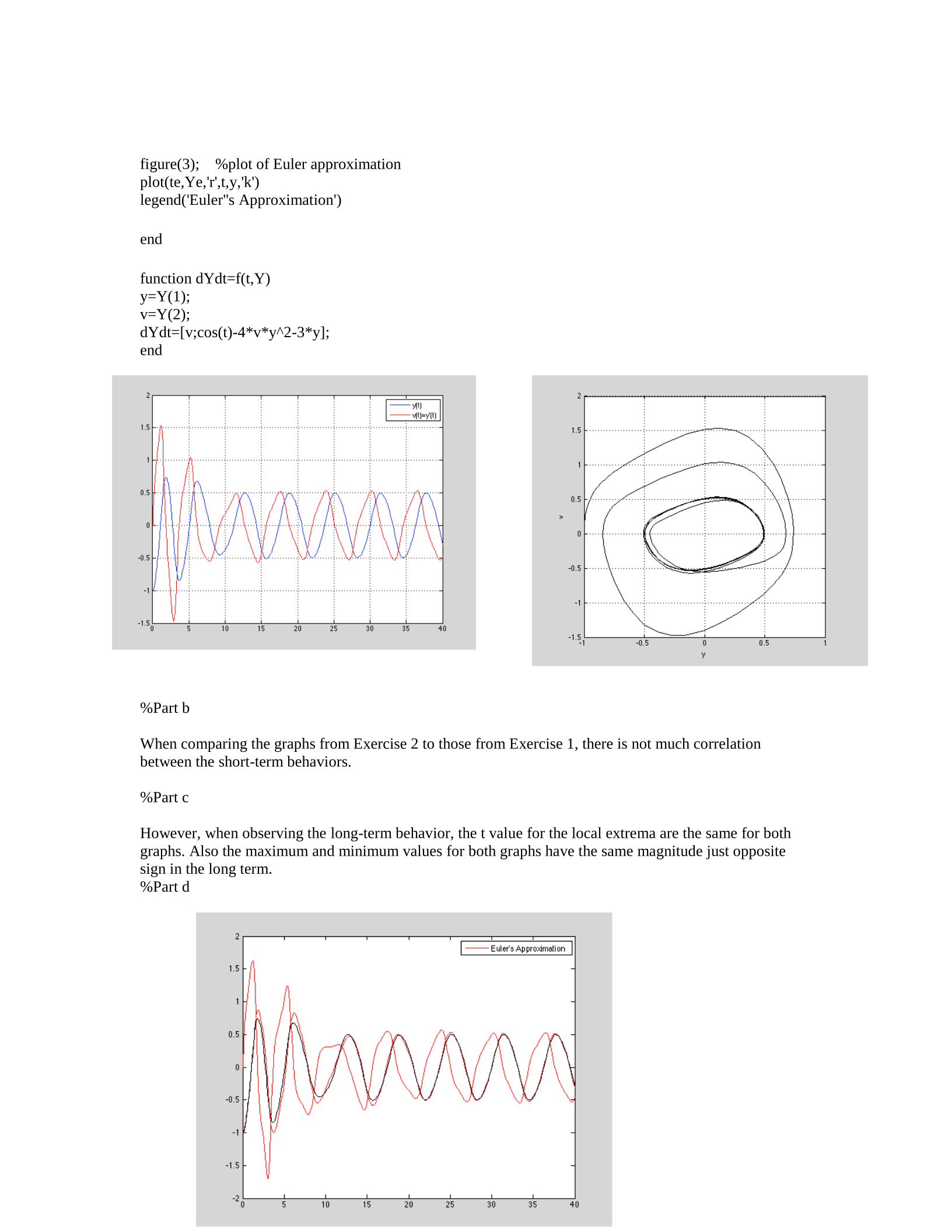
figure(3); %plot of Euler approximation
plot(te,Ye,'r',t,y,'k')
legend('Euler''s Approximation')
end
function dYdt=f(t,Y)
y=Y(1);
v=Y(2);
dYdt=[v;cos(t)-4*v*y^2-3*y];
end
%Part b
When comparing the graphs from Exercise 2 to those from Exercise 1, there is not much correlation
between the short-term behaviors.
%Part c
However, when observing the long-term behavior, the t value for the local extrema are the same for both
graphs. Also the maximum and minimum values for both graphs have the same magnitude just opposite
sign in the long term.
%Part d

%Exercise 3
function LAB4ex3C
t0=0;
tf=40;
Y0=[-1;0];
[t,Y]=ode45(@f,[t0,tf],Y0);
y=Y(:,1);
v=Y(:,2);
figure(1);
plot(t,y,'b-+',t,v,'ro-')
legend('y(t)','v(t)=y''(t)')
grid on;
ylim([-2,2]);xlim([0,40]);
figure(2);
plot(y,v)
axis square;
xlabel('y'); ylabel('v');
grid on
end
function dYdt=f(t,Y)
y=Y(1);
v=Y(2);
dYdt=[v;cos(t)-4*v*y-3*y];
end
The behavior of these solutions in Exercise 3 are significantly different than the solutions in Exercise 2.
The graphs do not resemble each other.
MATLAB does give a warning message :
Warning: Failure at t=3.774765e+00. Unable
To meet integration tolerances without reducing
the step size below the smallest value allowed
(7.105427e-15) at time t.
> In ode45 at 309
The warning means that at that point, the problem is stiff, because it is varying very slowly
%Exercise 4
%Part a
function LAB4ex4d
t0=0;
tf=40;
Y0=[-1;0;4]
[t,Y]=ode45(@f,[t0,tf],Y0);
y=Y(:,1);
v=Y(:,2);

w=Y(:,3);
figure(1);
plot(t,y,'b-+',t,v,'ro-',t,w,'k')
legend('y(t)','v(t)=y''(t)','w(t)=y''''(t)')
grid on;
ylim([-1.5,1.5]);
figure(2);
plot3(y,v,w,'k.-');
axis square;
xlabel('y'); ylabel('v=y'''); zlabel('w=y''''')
grid on
view([-40,60])
end
function dYdt=f(t,Y)
y=Y(1);
v=Y(2);
w=Y(3);
dYdt=[v;w;-sin(t)-4*y^2*w-8*y*v^2-3*v];
end

%Part b
Upon inspection, when comparing the wave graph from Part(a)with the wave graph from Exercise 2Part
(a), it can be seen that two of the time series graphs are exactly the same. In this case, the red graphs from
each and the blue graphs from each correspond with each other respectively.
%Part c
The derivative of the ODE is 𝑑3𝑦
𝑑𝑡3+ 4𝑦2𝑑2𝑦
𝑑𝑡2+ 8𝑦(𝑑𝑦
𝑑𝑡)2+ 3𝑦 𝑑𝑦
𝑑𝑡
%Part d
The derivative of the first ODE is dependent on the solution of the second ODE.
Powered by TCPDF (www.tcpdf.org)

