INTRODUCTION Illegal online sales have

Illegal online sales have grown exponentially [1]. Vendors can sell illicit products

through cryptomarkets or encrypted IM messages software like telegram easily. In darknet,

the privacy of participants in illicit online transactions is protected through both Tor and

cryptocurrency. The darknet utilizes The Onion Router (Tor) network to hide users’ IP

addresses from the internet service provider. Darknet markets choose cryptocurrencies as

payment currency mainly because they are anonymous. Unlike traditional currencies,

cryptocurrencies like Bitcoin are decentralized[2]: there is no central authority responsible

for the issuance of cryptocurrencies and there is no need to involve a trusted third-party like

banks when making online transfers [3,4]. Both buyers and vendors can trade anonymously

through cryptocurrencies [5]. For IM software like telegram, they provide encryption

services for users. Users of IM applications can easily hide their identities while interacting

with strangers online. The privacy provided by darknet and IM software make it hard for law

enforcement to trace illicit business online. This fact inspires us to conduct the research to

extract useful information from public data in these platforms through data mining

algorithms to combat cyber crime.

We first investigate the characteristics of Bitcoin transactions behind cryptomarkets in

part 2. Darknet utilized the decentralized cryptocurrencies as payment currency. We conduct

transactions on different types of markets to discover the currency management of

cryptomarkets. In part 3, we further propose a method to identify vendors’ Bitcoin addresses

by matching vendors’ feedback reviews with Bitcoin transactions in the public ledger. Each

feedback review is matched to a Bitcoin transaction based on timestamp and value

transferred in this transaction. Therefore a Bitcoin address whose history transactions can

match more reviews of a vendor have a higher possibility to belong to this vendor. In part 4,

we propose a model to discover hidden influence networks between members in a group

chat. We can model message sequences to a Temporal-Textual Multi-Dimensional Hawkes

process and learn the Granger Causality between different individuals. In part 5, we propose

a model to cluster the accounts that belong to the same user in IM software. We design a 24-

7 CNN to learn the representations of timestamp lists. By leveraging the post and time pattern

of accounts, we propose a method to learn the embedding of each account and train a binary

classifier to identify accounts from the same user.

1.1 Background

In this chapter, we provide the background information of our topic, including Darknet,

Bitcoin, and Hawkes Process respectively.

1.1.1 Darknet

A darknet market is a commercial website on the dark web that operates via darknets

such as Tor. They function primarily as black markets, selling or brokering transactions

involving drugs, weapons, counterfeit currency, stolen credit card details, forged documents,

unlicensed pharmaceuticals, steroids and other illicit goods as well as the sale of legal

products. Tor is a network of virtual tunnels that allows you to improve your privacy and

security on the Internet. Tor works by sending your traffic through three random relays in

the Tor network. The last relay in the circuit (the “exit relay”) then sends the traffic out onto

the public Internet. Tor provides hidden services (also known as onion services) for users to

hide their locations and identities while offering web publishing services. Vendors and

buyers can surf the darknet through Tor browser without leakage of their IP addresses to

internet service providers.

1.1.2 Bitcoin

Bitcoin is the first decentralized cryptocurrency (also known as digital currency or

electronic cash) that operates on the peer-to-peer network without the need for

intermediaries and there are no central banks or administrators. Transactions are verified by

network nodes via cryptography and recorded in a public distributed ledger called a

blockchain. Users can transfer Bitcoin pseudonymously because funds are not tied to real-

world entities but rather bitcoin addresses. Owners of bitcoin addresses are not explicitly

identified. We focus on Bitcoin in this dissertation because Bitcoin is the most popular

cryptocurrency which is accepted by all darknet markets [6]. Using blockchain and

distributed ledger technology, the Bitcoin system promises great transparency and improved

trust across transaction value chains [7,8]. Without a third-party to ensure a transaction, the

Bitcoin system publishes all of its history transaction data. The Bitcoin ledger stores all

transaction records in history which are public to any Bitcoin users. A user wallet can own

multiple bitcoin addresses, which are the “pseudonymous identity” of this user in the public

ledger.

1.1.3 Hawkes Process

One-dimensional Hawkes process is a type of temporal point process which can model

the self-exciting event sequence. The intuition behind it is that previous events may trigger

the occurrence of future events. A temporal point process can be represented as a counting

process, N = {N(t)|t ∈ [0,T]}, where N(t) records the number of events before time t. Intensity

function λ(t) = E[(dN(t)|H)]/dt represents the expected instantaneous happening rate of

event given the event history H. Due to self-excitation, the intensity function of Hawkes

process is conditionally based on history events. Given a sequence of n events on time T =

{t1,t2,t3...tn}, officially the intensity function of event in Hawkes process is

λ(t) = µ + X α · g(t − tj) (1.1)

j:tj<t

where µ is exogenous base intensity independent of history while the second part on the right

side is impact from previous events. tj is the occurrence time of a previous event. g(∆t) is the

triggering kernel which decays with time difference. The earlier the previous event, the less

impact it has on the current event. α is a coefficient measuring the amount of influence from

previous events on the current event. Here we use an exponentially decaying function to

capture the influence.

g(ti − tj) = βe−β(ti−tj) (1.2)

1.2 Characteristics of Bitcoin Transactions on Cryptomarkets

The darknet is a portion of the Internet that purposefully protects the identities and

privacy of both web servers and clients. The Onion Router (Tor) is the most popular instance

of a darknet and also the most popular anonymous network. A cryptomarket (or darknet

market) is a commercial website operating on the darknet. Specifically, in Tor, a cryptomarket

is a hidden service website with a “.onion” link address. Most products being sold in

cryptomarkets are illicit. Some examples of popular products in cryptomarkets are drugs,

malware, and stolen credit cards. After the demise of the first cryptomarket called Silk Road

in 2013, new cryptomarkets have proliferated. Bitcoin is accepted in all cryptomarkets. As

the first decentralized cryptocurrency, Bitcoin operates on the peer-to-peer network without

the need for intermediaries and there are no central banks or administrators. In this section,

we systematically study the vulnerabilities of Bitcoin privacy that exist in cryptomarkets. We

identify and categorize patterns of Bitcoin transactions in cryptomarkets. The observations

are then used for discussing the possibility of re-identifying Bitcoin addresses related to

cryptomarkets. The conclusions obtained from this chapter can help design better Bitcoin

payment systems and strengthen the privacy protection. On the other hand, the conclusions

can also be used by law enforcement to understand the activities in cryptomarkets.

1.3 Identifying Darknet Vendor Wallets by Matching Feedback Reviews with Bitcoin

Transactions

In part 3, we aim at finding vendors’ Bitcoin addresses used in the darknet markets by

matching feedback reviews with Bitcoin transactions. To narrow down the scope of the

problem, we choose Bitcoin and Wall Street Market as a study example. Each feedback review

is matched to a Bitcoin transaction based on timestamp and value transferred in this

transaction. Specifically, we decompose our problem formulation into two sub-problems:

Bounding Box Matching Problem and Maximum Review Coverage Problem. In the Bounding

Box Matching Problem, we construct a bounding box for each review and find matched

Bitcoin transactions. We build a K-D tree from massive Bitcoin transaction data to achieve

quick range searching in a bounding box. In the Maximum Review Coverage Problem, we

prove the NP-Hardness of the problem. We exploit the submodular property of the objective

function and design a greedy algorithm with an approximation ratio of (1 − 1/e) to find a set

of addresses that can cover near-optimal product reviews received by one vendor. Our

method can discover the number of addresses used by one vendor, realizing one-to-many

mapping. We further develop an algorithm that can effectively accelerate the matching and

greedy algorithm.

Our contributions are as follows:

• We propose the problem of identifying the vendors’ Bitcoin addresses by matching

public Bitcoin transactions to vendor’s feedback reviews in darknet markets. This

problem is important because of two potential applications. First, it helps law

enforcement to trace illicit transactions. Second, it reveals a privacy concern of

cryptocurrencies so helps better design new cryptocurrencies.

• We decompose the complicated problem into two sub-problems and provide efficient

computing algorithms for the sub-problems. We further propose a Cost-Effective

Addresses Searching(CEAS) algorithm to accelerate the whole process, which can

reduce about 60% matching calculations in experiments.

• We extensively evaluate our methods in both real and synthetic data and demonstrate

the effectiveness and accuracy of our method.

1.4 Learning Infectivity Graph in Chat Group via Temporal Textual Multidimensional

Hawkes Process

Instant message(IM) applications provide a convenient way for people to communicate

and exchange confidential information. Users of IM applications can easily hide their

identities while interacting with strangers online. To protect user’s privacy, some IM

developers provide encryption services for their customers. However, these privacy-

protecting and convenient software has been utilized by criminals for illegal activities like

drug smuggling, online fraudulence or even anti-social activities[9].

In part 4, we propose a framework which extracts the weighted directed infectivity

graph by applying data mining and natural language processing techniques on the chat log of

a group. The chat history is a sequence of messages where each message contains

information including time when the message is posted, members who post the message and

text content. The timestamp of each message makes chat history a time series data, which

can be viewed as event sequences containing multiple event types and modeled via multi-

dimensional point processes. Each posted message can be viewed as an event with a

timestamp and the person’s identity can represent the corresponding event type. To

construct Granger Causality graph over event types(members in group), we model the data

with a special class of point processes called Hawkes processes. Hawkes Process is a type of

temporal point process which is widely used to model the self-exciting event sequences like

earthquakes. When there are multiple event types, Hawkes Process is capable of describing

mutually-triggering patterns among different event types. We relate influence between users

to the possibility of replies among members. Natural language processing techniques are

utilized to find dialogues in group chat logs. Impact functions of Hawkes process can capture

the influence graph.

Our contributions are as follows:

• We propose the problem of detecting the influence graph from group chat. It helps law

enforcement to analyze the organizational structure and key person from criminal

activities in group chat.

• We present a modeling framework based on text biased Marked Multi-dimensional

Hawkes Process. Hawkes Process can extract mutual-triggering patterns over

individuals in a group. We further apply natural language processing techniques to

identity conversations from the chat log and update impact functions of Hawkes

process with the reply embedding. By applying an EM algorithm on the model, we are

able to learn the influence graph over individuals from chat logs.

1.5 Clustering of Accounts in Online Messaging Software through Attributed

Heterogeneous Information Networks

In this work, we propose a model to learn the representations of each account in group

chat through attributed heterogeneous information networks.

The aim of this work is to cluster users based on time pattern and text of the post. The

intuition behind our method is that if a vendor has several accounts, he or she will post the

similar content with a similar time pattern by using these accounts.

Our contributions are as follows:

• We present a model to learn the representations of time stamp series by training a CNN

auto-encoder. The embedding we learned can be used to measure the similarity of two

timestamp lists effectively.

• We build an Attributed Heterogeneous Information Network. In the AHIN we built, it

contains four types of nodes: User, account, post and product. We train a model to learn

the embedding of each node. To effectively measure the relationship between nodes in

constructed AHIN, we sample paths from AHIN through weighted random walk and

propose a new network embedding model User2Vector to learn the hidden

representations of each user. We further train a binary classifier to classify two user

representations we learned by User2Vector.

• We extensively evaluate our methods in both real and synthetic data and demonstrate

the accuracy of our method.

1.6 Proposed Dissertation Organization

In this dissertation proposal, we plan to investigate how to efficiently extract useful

information from darknet and IM software. In part 2, we describe our experiments of

purchases in cryptomarkets and summarize the Bitcoin transaction mechanisms behind

cryptomarkets. In part 3, we present a greedy method to identify vendors’ bitcoin addresses

by matching vendors’ feedback reviews with Bitcoin transactions in the public ledger. In part

4, we present our work which models group chat with Hawkes Process to discover hidden

networks of influence between members. In part 5, we propose a model to cluster the

accounts from the same user by learning the embedding of these accounts. In part 6, we

conclude this

dissertation.

PART 2

CHARACTERISTICS OF BITCOIN TRANSACTIONS ON

CRYPTOMARKETS

In this chapter, we discover interesting characteristics of Bitcoin transaction patterns in

cryptomarkets. The results demonstrate that the privacy protection mechanism in

cryptomarkets and Bitcoin is vulnerable.

2.1 Motivation

Illegal online sales have grown exponentially [1]. The privacy of participants in illicit

online transactions in darknet is protected through both Tor and cryptocurrency. Vendors in

cryptomarket sell illicit products like drugs, malware, and stolen credit cards. The sales on

the darknet market hit a new high in 2021 although the law enforcement has spent a lot of

resources to fight these illegal transactions.

Table (2.1) Cryptomarkets and Accepted Cryptocurrencies

Cryptomarkets

#Ads

Bitcoin

Monero

Litecoin

Ethereum

Bitcoin Cash

Dream

166,216

Berlusconi

38,462

Wall Street

16,847

Empire

9,538

Point Tochka

6,468

Silk Road 3.1

5,738

From Table 2.1, we can see that Bitcoin is accepted in all cryptomarkets. In addition to

Bitcoin, four other types of cryptocurrencies are also accepted by different markets. They are

monero, litecoin, ethereum, and Bitcoin cash. Note that Bitcoin cash is a variant of but

different from Bitcoin and is an independent currency. Bitcoin cash is generally considered

to be faster in the transaction confirmation process but less secure than Bitcoin. In our study,

we focus on Bitcoin since it is the most popular cryptocurrency and widely accepted by all

markets. The observed Bitcoin transaction patterns in this chapter provide insights for

analyzing other types of cryptocurrencies.

Since all Bitcoin transactions are public, it is hard to fully protect the privacy of Bitcoin

users. The news has revealed that adversaries could spy on a careless company by first paying

it in Bitcoins and then tracking how that money flows [10–12]. To better protect the privacy,

Bitcoin users have extensively used mixing services to obscure the Bitcoin trails [10].

Figure (2.1) The Feedback in the Dream Market

In cryptomarkets, adversaries could place orders and then track money flows.

Cryptomarkets display the buyers’ feedback in order to demonstrate the vendors’ reputation.

Figure 2.1 shows the screenshot of the feedback page in the Dream Market. From Figure 2.1,

we can see the post time, rating star, text comment, masked buyer ID, and approximate

amount of money. Each rating actually represents a Bitcoin transaction. Even though we can

only observe approximate time and money in ratings, the accumulation of a lot of such

approximate transaction records could potentially allow adversaries to reveal relevant

Bitcoin addresses. Figure 2.2 shows the screenshot of the feedback page in the Wall Street

Market. From Figure 2.2, we can observe similar ratings. All markets in Table 2.1 display

feedback publicly. This potentially allows adversaries to re-identify the Bitcoin addresses of

buyers, vendors, and escrow accounts in cryptomarkets, thus increasing the vulnerability of

Figure (2.2) The Feedback in the Wall Street Market

the privacy protection in Bitcoin.

2.2 Related Work

Ron et al. is the first to build a Bitcoin graph and analyze the quantitative attributes in

Bitcoin transaction history [13]. Clustering Bitcoin addresses into wallets is one basic task in

the Bitcoin transaction analysis. Researchers have widely used two simple heuristics [14–

16]. The first heuristic is to put shadow or change address together with its input address

into one wallet. The second heuristics is to put all input addresses into one wallet if there is

a single output address. Androulaki et al. test the effectiveness of the Bitcoin address

clustering methods with stimulations [14]. Spagnuolo et al. link the clustered wallets to the

Silk Road escrow addresses exposed by FBI and analyze the Bitcoin flow [15]. Fleder et al.

not only link the clustered wallets with Silk Road escrow but also link wallets with public

wallets [16]. PageRank is then applied on the transaction graph to find interesting and

important wallets [16]. The effectiveness of address clustering is also studied [17]. Mixing

technology is also introduced to improve the anonymity [18,19].

2.3 Escrow Services in Cryptomarkets

In this section, we review the escrow services in cryptomarkets. All cryptomarkets

provide escrow services to avoid scams and protect both buyers and vendors.

Figure (2.3) A Flowchart Depicting a Transaction in Cryptomarkets

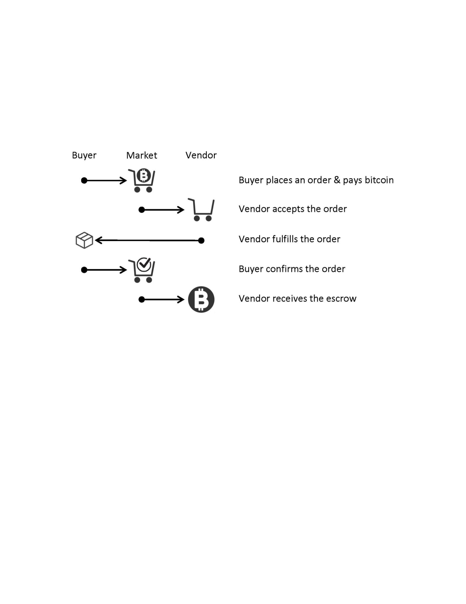
Figure 2.3 shows the typical process of one transaction [20]. The buyer places an order

and pays with Bitcoins after browsing the products within the Tor web browser. The market

holds the Bitcoins until the buyer confirms the order. The vendor accepts and fulfills the

order. The buyer confirms the order and gives feedback reviews. The market releases the

Bitcoins to the vendor and charges a commission fee. If the buyer is not satisfied with the

product or service, the buyer disputes the order. In this case, the market decides where the

escrow Bitcoins go. The escrow Bitcoins go either back to the buyer or to the vendor

depending on the dispute result.

2.4 Bitcoin Transactions

2.4.1 Parsing Bitcoin Transactions

To trace the Bitcoin flow, we parse the blocks in the public Bitcoin blockchain and obtain

the Bitcoin transactions. We install the Bitcoin core program [21] and run a Bitcoin full node

[22]. The Bitcoin full node automatically synchronizes with other nodes in the Bitcoin

network, and downloads all blocks in the blockchain. The blocks contain the public ledger

data and are the inputs of our parsing algorithm. A new block is generated around every 10

minutes.

Algorithm 1 Parsing Bitcoin Transactions

Input: Blocks in the Bitcoin blockchain

Output: Bitcoin transactions (a set of .json files whose names are formatted timestamps) for

each block do transaction time ⇐ block.timestamp; create a new file: formatted

transaction timestamp.json; for each transaction in the block.transactions do transaction

hash ⇐ transaction.this transaction hash; receiver list = [] ; for each receiver in the

transaction.receivers do receiver list.add(receiver.index, receiver.Bitcoin address,

receiver.Bitcoin value)

sender list = [] ; for each sender in the transaction.senders do sender

list.add(sender.index, sender.previous transaction hash,

sender.previous transaction index)

[transaction time, transaction hash, sender list, receiver list] ⇒ formatted

transaction timestamp.json

Algorithm 1 shows our parsing algorithm. We use the existing Python Bitcoin parser to

parse the blocks (raw Bitcoin data) and construct the Bitcoin transaction tree [23,24]. In

Algorithm 1, we parse the blocks one by one (lines 1-12) and save one timestamp for all

transactions in one block (line 2). For each transaction in one block, we parse the transaction

hash (line 5), the receiver list (lines 6-8), and the sender list (lines 9-11). Each transaction

contains four parts: timestamp, hash, sender list, and receiver list, and is written into a

Algorithm 2 Constructing Bitcoin Transaction Flow Tree

Input: Bitcoin transactions (a set of .json files whose names are formatted timestamps)

Output: Bitcoin transaction flow tree G(V,E) read the list of json files; for each json file (process them

in the chronological order) do

read all transactions in the json file;

json file (line 12). One receiver contains the Bitcoin address and the Bitcoin values. Each

sender in one transaction does not contain a Bitcoin address nor Bitcoin value. Instead, each

sender contains transaction hash and index pointing to an earlier transaction. We can use

that transaction hash to retrieve the earlier transaction and use the transaction index to find

the referred receiver from the receiver list. By linking the sender in the current transaction

with the receiver in the earlier transaction, we can generate a Bitcoin transaction flow tree.

Algorithm 2 shows the construction of the Bitcoin transaction flow tree. Algorithm 2

processes the json files in the chronological order. This guarantees that old transactions will

be processed earlier than new transactions. Since a receiver has a Bitcoin address, we can

directly add a node (transaction hash, Bitcoin address) to the flow tree. Since a sender does

not have a Bitcoin address, we need to look it up in an earlier transaction. Since earlier

transactions have been processed, the sender must exist in the node set V as a receiver.

Therefore, we search over all the nodes in V and compare the transaction hash and index

values (lines 8). Then we add an edge from this earlier receiver to the current receiver in the

flow tree. If there are multiple senders and receivers in a mixing transaction, these senders

and receivers will form a complete bipartite graph, i.e., there is an edge from any sender to

any receiver. We do not know who sends money to whom in a mixing transaction.

Algorithm 3 Local Search Algorithm for Extracting a Subtree

Input: Bitcoin transaction flow tree G(V,E), query q = (q hash,q btc address), k hops

for

eachtransactiontx

for

eachreceiverintx.receiver

list

addnode

tx.transaction

hash,receiver.index,receiver.Bitcoin

address,

receiver.Bitcoin

value]tothenodeset

;

for

eachsenderintx.sender

list

findnode

∈

with

.transaction

hash=sender.previous

transaction

hash

and

.index=sender.index;

addanedge(

s,r

)

totheedgeset

;

Output: Subtree G[T] ignore the edge direction, G.Adj[u]

represents the neighbors;

for each node v ∈ V do v.d = ∞ ;

Algorithm 3 shows a local search algorithm that retrieves a subtree containing all nodes

that are k-hop away from the query node. The query node is determined by the transaction

hash and Bitcoin address. In our experiment, we use Algorithm 3 to extract a subtree given a

query node containing our Bitcoin address. The subtree is nimble for us to analyze

interesting patterns.

Shadow Address: Bitcoin creates a new address for the sender in each transaction to

obtain better anonymity [25]. The newly generated address is called “shadow address” or

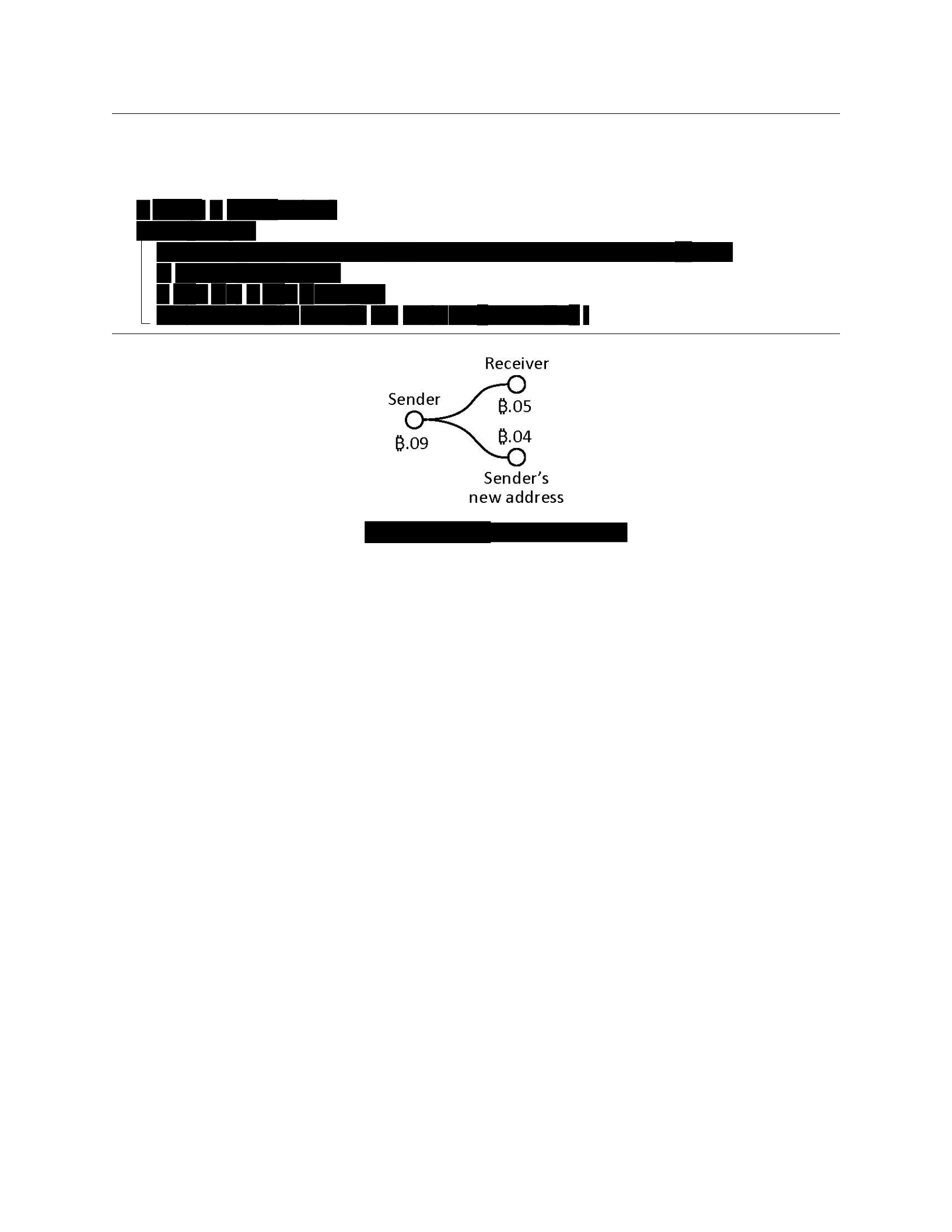
“change address” of the original address of the sender [14]. Figure 2.4 shows one Bitcoin

transaction. The sender’s original address has .09. After .05 is sent to the receiver, the sender

still has .04 in the change address.

Multiple inputs and single output: Considering the multiple addresses one user can own,

Bitcoin supports a user to send Bitcoins from multiple addresses in one transaction. Figure

2.5 shows one Bitcoin transaction containing multiple inputs and one output. The sender

sends money from four Bitcoin addresses to the receiver’s address. We assume that it is

⇐{

}

;

⇐{}

;

q.d

;

while

True

extractnode

withminimum

u.d

valueamongallnodesintheset

−

;

u.d>k

then

break;

⇐

∪

;

⇐

∪

G.Adj

[

]

;

for

eachnode

G.Adj

[

]

x.d

min

{

x.d,u.d

}

;

Figure(2.4)

ShadowAddress

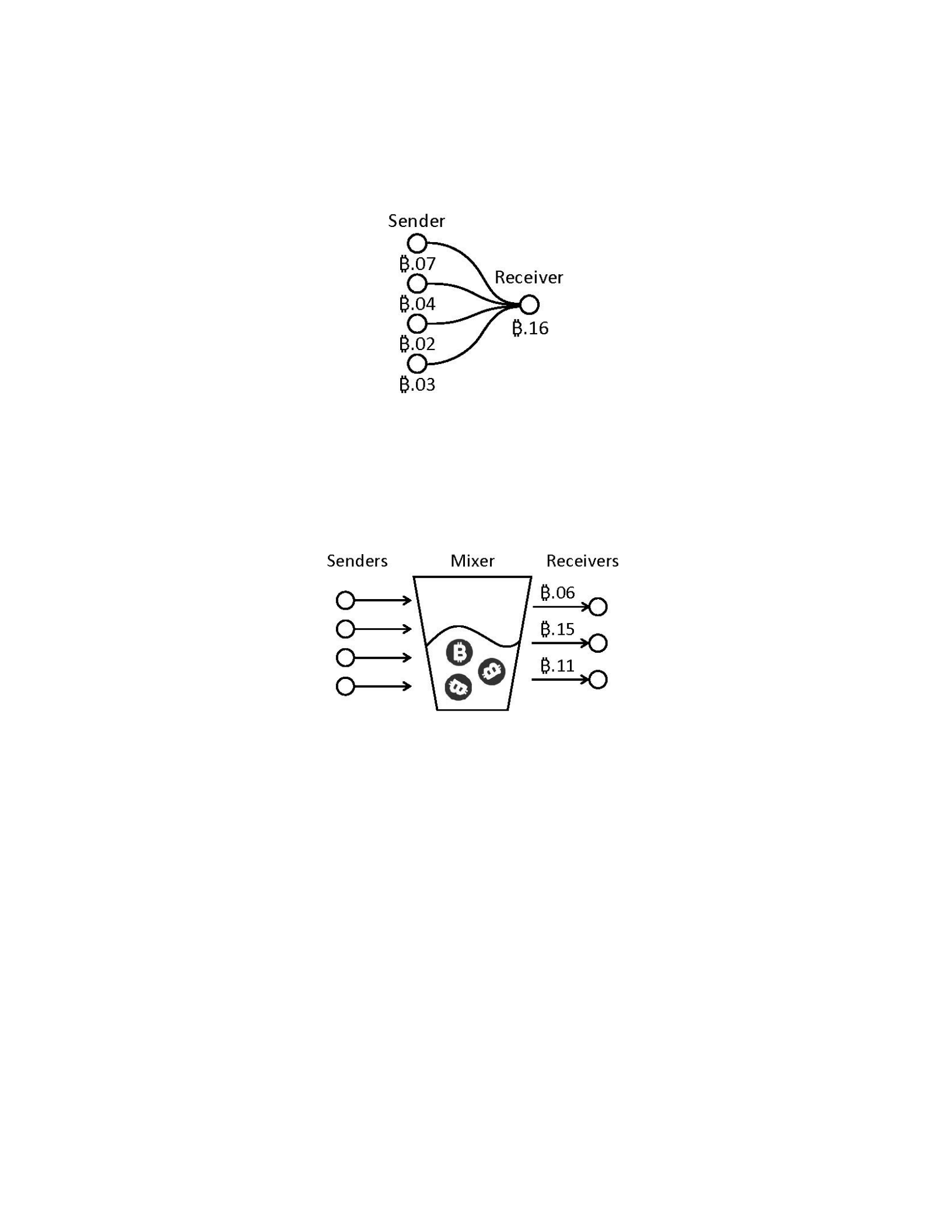
unlikely that two senders send money to the same address at the same time since the Bitcoin

addresses keep changing. If we observe a transaction with multiple inputs and single output,

we can assume all input addresses belong to the same sender.

Figure (2.5) Multi-Inputs

These two properties help track Bitcoin flows or cluster addresses into wallets [14,16,26].

Figure (2.6) A Mixing Transaction

Mixing services: are widely used as a privacy overlay on top of Bitcoin [27]. Mixing

services are also known as tumblers. The mixer will mix several transactions into one,

intending to confuse the trail linking back to the source. In a mixing transaction, the multiple

inputs are from different senders and the multiple outputs go to different receivers. Mixing

services reduce the traceability of Bitcoin flows which makes the analysis of Bitcoin graphs

more difficult. Figure 2.6 shows a mixing transaction with four senders and three receivers.

In this example, we do not know who sends money to whom because there are

multiple possible flows.

2.4.2 Actions and Observed Resulting Transactions

In this section, we describe our experiments in cryptomarkets. All cryptomarkets offer

escrow services to avoid scams. With the escrow service, the Bitcoin is saved in escrow

accounts after a buyer places an order and is sent to the vendor until the buyer confirms the

order. Since we know the start point (buyer address) of the transaction, we can trace Bitcoin

flows to uncover escrow and vendors’ addresses.

Table (2.2) Observed Bitcoin Flow from Operations in Different Cryptomarkets

Cryptomarkets

Deposit

Withdraw

Order

Confirm

Point Tochka

Dream

No observation

Empire

No observation

Silk Road 3.1

No observation

Wall Street

No such function

Berlusconi

No such function

No observation

In each market, four operations are performed: deposit, withdraw, order, and

confirmation. The resulting transactions may or may not be observed in the Bitcoin

transaction flow. Table 2.2 shows whether we can observe the Bitcoin transactions for the

four operations in cryptomarkets. From Table 2.2, we can see that the Dream, Empire, and

SilkRoad 3.1 Market operate in a similar way. These markets require buyers to deposit

Bitcoins first. When buyers withdraw Bitcoins from the market, the market will send Bitcoins

to buyers’ wallets from an address different from the deposit address. When we order or

confirm a purchase, we cannot observe any transactions in Bitcoin flow. The Point Tochka

Market also requires a deposit. When we order and confirm a purchase in the Point Tochka

Market, we can observe the transactions from buyer to escrow and then to vendor in the

Bitcoin flow. The Wall Street and Berlusconi Markets do not require deposit. In the Wall street

Market, when we order and confirm a purchase, we can also observe the corresponding

transactions in the Bitcoin flow. In the Berlusconi Market, we can observe the transactions in

Bitcoin flow when we order. The Bitcoins sent to escrow are transferred to other escrow

addresses through a mixing service before we confirm the purchase. Therefore, we cannot

observe the transaction when we confirm the purchase.

Table (2.3) Deposit and Withdrawal in the Point Tochka Market

Action

Observed Bitcoin transaction

Balance

Sender

Receiver

Deposit .0024

A1: .0030

B1: .0024, A2: .0006

.0024

Withdraw .0008

B1: .0024

A2: .0008, B1: .0016

.0016

Deposit .0010

A2: .0006, A2: .0008

B1: .0026, A3: .0004

.0026

Withdraw .0006

B1: .0026

A3: .0006, B1: .0020

.0020

In the next, we will study the Bitcoin transaction patterns when we interact with the

markets. We first study the deposit and withdrawal actions and then the order and

confirmation actions. In each market, four operations are performed: deposit .0024,

withdraw .0008, deposit .0010, and withdraw .0006. We monitor the Bitcoin transaction flow

to see whether we can observe any related transactions or not. To simplify the illustration,

we omit the fees charged during the deposit and withdrawal actions.

Deposit and Withdrawal in the Point Tochka Market: Table 2.3 shows the actions we

perform and the resulting Bitcoin transactions in the Point Tochka Market. In

Table 2.3, each row represents an action we perform and the resulting Bitcoin transaction.

We use letter “A” followed by an integer to represent our Bitcoin addresses and letter “B”

followed by an integer to represent the deposit Bitcoin addresses provided by the market.

For example, in the first row, we deposit .0024 and the resulting transaction is “A1: .0030

→ B1: .0024, A2: .0006”. In the sender part “A1: .0030”, A1 represents our Bitcoin address and

.0030 represents the money in that address. In the receiver part “B1: .0024, A2: .0006”, B1

represents the deposit Bitcoin address provided by the Point Tochka Market,

.0024 represents the money that B1 receives, A2 represents our new Bitcoin address, and

.0006 represents the change in the new address A2. The last column in Table 2.3 shows the

balance in the market wallet.

In the second row of Table 2.3, we withdraw .0008 and the resulting transaction is “B1:

.0024 → A2: .0008, B1: .0016”. B1 still represents the deposit Bitcoin address and A2 still

represents our Bitcoin address for receiving the money. We further deposit .0010 and

withdraw .0006, and the resulting transactions are shown in Table 2.3.

From Table 2.3, we can see that the deposit Bitcoin address in the market does not

change. Among all cryptomarkets in Table 2.1, the Point Tochka Market has the most

transparent Bitcoin transaction flows, which can be further confirmed when we study the

order and confirmation actions.

Table (2.4) Deposit and Withdrawal in the Dream Market

Action

Observed Bitcoin transaction

Balance

Sender

Receiver

Deposit .0024

A1: .0030

B1: .0024, A2: .0006

.0024

Withdraw .0008

B2: .0008

A2: .0008

.0016

Deposit .0010

A2: .0006, A2: .0008

B3: .0010, A3: .0004

.0026

Withdraw .0006

B4: .0006

A4: .0006

.0020

Deposit and Withdrawal in the Dream Market: We perform the same sequence of

actions in the Dream Market and Table 2.4 shows the resulting transactions. From Table 2.4,

we can see that the Bitcoin address B2 that sends us money during the first withdrawal is

different from the Bitcoin address B1 that receives our money during the first deposit. After

the second withdrawal, we find that there is still .0024 in B1. This means that the Dream

Market uses different Bitcoin addresses to receive deposits and send withdrawal. From the

subsequent deposit and withdrawal actions, the deposit is sent to B3 and the withdrawal is

received from B4. This further confirms the observation. This mechanism makes it harder to

track the Bitcoin flow, thus better protects the privacy of the market and prevents the

re-identification attack.

The Empire and Silk Road 3.1 Markets have similar transaction patterns as Dream

Market for the deposit and withdrawal actions. We omit the tables for them. The Wall Street

and Berlusconi Markets provide neither deposit nor withdrawal functions. They allow buyers

to directly pay from their own Bitcoin addresses.

In the next, we study patterns in the resulting Bitcoin transactions for the order and

confirmation actions.

Table (2.5) Order and Confirmation in the Point Tochka Market

Action

Observed Bitcoin transaction

Balance

Sender

Receiver

Order .0014

B1: .0040

C1: .0014, B1: .0026

.0026

Confirm

C1: .0014

D1: .0014

.0026

Order .0015

B1: .0026

C2: .0015, B1: .0011

.0011

Confirm

C2: .0015

D2: .0015

.0011

Order and Confirmation in the Point Tochka Market: We purchase two orders and

Table 2.5 shows the resulting Bitcoin transactions. After we place the first order, the money

is sent from the deposit Bitcoin address B1 to an escrow account C1. The balance is sent back

to B1. After the vendor fulfills the order, we confirm it. The money in the escrow C1 is then

immediately transferred to a new Bitcoin address D1, which is suspected of being the

vendor’s Bitcoin address. In the second order, we pay 0.0015 to a different vendor. Similar to

the transactions in the first order, the money moves to an escrow account C2 after the order

and then moves from C2 to the destination Bitcoin address after confirmation. The escrow

address C2 is different from the old escrow address C1. From this experiment, we can see

that the Bitcoin transaction flows are transparent. For each new order, the market will

generate a new escrow Bitcoin address. We also observe that our deposit Bitcoin address will

not change. By tracking the money flowing out of the escrow accounts, we can potentially

find the suspicious Bitcoin addresses of vendors.

Order and Confirmation in the Dream Market: We also purchase two products in the

Dream Market and Table 2.6 shows the resulting transactions. After we place the first order

of 0.0014, we find that no transaction associated with the deposit Bitcoin address Table (2.6)

Order and Confirmation in the Dream Market

Action

Observed Bitcoin transaction

Balance

Sender Receiver

Order .0014

B1: .0040 does not change

.0026

Confirm

B1: .0040 still no change. No transactions observed

.0026

Order .0015

B1: .0040 does not change

.0011

Confirm

B1: .0040 still no change. No transactions observed

.0011

B1 happens. After the vendor fulfills the order and we confirm it, still nothing happens. This

means Dream Market uses a different escrow Bitcoin address to pay the vendor and the

money in the original deposit address B1 does not move. Since we know neither the escrow

address used to pay the vendor nor the vendor Bitcoin address, there is no easy way for us to

observe the relevant transactions. We suspect that the Dream Market has its own private

ledger to record the balances of the deposit and escrow accounts for each user. After each

order, the Bitcoin in the deposit account will be transferred to the escrow account. After each

confirmation, the Bitcoin in the escrow account will be transferred out to the vendor’s

accounts. The ledger of Dream Market might be a private and centralized ledger. This strategy

makes the transactions within the Dream Market stealthy and cannot be seen from the public.

This strategy well protects the privacy of the market and vendors.

Table (2.7) Order and Confirmation in the Wall Street Market

Action

Observed Bitcoin transaction

Sender Receiver

Order .0014

A1: .0040 C1: .0014, A2: .0026

Confirm

C1: .0014 is transferred to another address through mixing

Order .0015

A2: .0026 C2: .0015, A3: .0011

Confirm

C2: .0015 is transferred to another address through mixing

Order and Confirmation in the Wall Street Market: The Wall Street Market does not

have a deposit function. It allows us to pay directly with our Bitcoin address. When we

purchase, we are required to send a specific amount of Bitcoin to a newly generated escrow

address and to provide a Bitcoin address for receiving the refund if the order fails. Following

this procedure, we purchase two products. Table 2.7 shows the resulting transactions. After

we place the first order, we can see the escrow address C1. After we confirm the order, we

can observe that the money in the escrow C1 is transferred to a new Bitcoin address through

a mixing service. Since there are multiple receivers, we do not know which one is the receiver

corresponding to the escrow C1.

Table (2.8) Order and Confirmation in the Berlusconi Market

Action

Observed Bitcoin transaction

Sender Receiver

Order .0014

A1: .0040 C1: .0014, A2: .0026

Confirm

C1: .0014 is transferred to another address through mixing

Order .0015

A2: .0026 C2: .0015, A3: .0011

Confirm

C2: .0015 is transferred to another address through mixing

Order and Confirmation in the Berlusconi Market: The Berlusconi Market does not

have a deposit function either. We directly pay with our Bitcoin address and Table 2.8 shows

the resulting transactions. After we place the first order, we can see the escrow address C1.

But before we confirm the order, the money in the escrow C1 is already transferred to a new

Bitcoin address through the mixing service. This makes it hard for us to track the Bitcoin

flows. Similar pattern is observed for the second order. The Berlusconi Market applies mixing

services on escrow addresses to further protect the privacy of the market and vendors.

Since the Wall Street and Point Tochka Markets provide more transparent Bitcoin

transaction patterns, the feedback reviews may help re-identify the Bitcoin addresses of

vendors. A feedback review is usually posted right after the buyer confirms the order. Each

review represents an approximate Bitcoin transaction including approximate date and

money.

We will see more details in the next sections.

2.5 Bitcoin Transaction Patterns

2.5.1 Dream Market

In this section, we track back the Bitcoin flows of the withdrawal operation in Dream

Market with Algorithm 3. We find a Bitcoin address containing more than 800 Bitcoins which

is worth over 3 million dollars at present, and it collects those Bitcoins from multiple

addresses in one transaction. Figure 2.7 shows part of the flow tree we observed. The red

node represents our Bitcoin address for receiving money in the withdrawal. We observe a

Bitcoin transaction pattern called “peeling chain” [26].

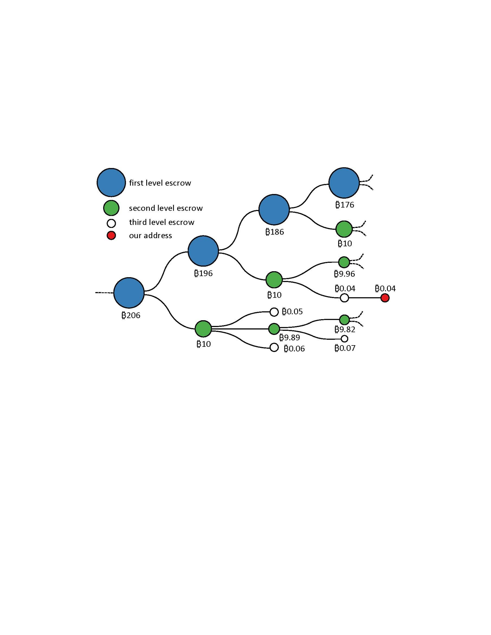
Peeling Chain: The head of a peeling chain is a Bitcoin address with a lot of Bitcoins. A

small amount of Bitcoin is peeled off from this address in a transaction and a ”Shadow

address” is generated to collect the remaining and still large amount of Bitcoin. By repeating

this process, the large amount of Bitcoin can be peeled down. Peeling chain is popular for

organizations dealing with a lot of clients. The Bitcoin addresses in a peeling chain are not

necessarily the addresses of Dream escrow accounts. They might be exchange addresses [28].

Figure (2.7) Bitcoin “peeling chain” Patterns in the Dream Market

The head of this peeling chain is a Bitcoin address which receives more than 800

Bitcoins. In each transaction, 10 Bitcoins are transferred to a new address and the remaining

amount is transferred to the shadow address. We call these blue addresses in the main chain

the first level escrow addresses. Each of the addresses containing 10 Bitcoins becomes a head

of a new smaller peeling chain. In this new chain, one transaction peels off an even smaller

amount of Bitcoin to pay different users. We call the green addresses in the smaller peeling

chains the second level escrow addresses. The Bitcoins peeled off from the second order

addresses are sent to third level escrow addresses, which are white nodes in Figure 2.7. The

white nodes directly send Bitcoins to users (red nodes) of the dream market. The amount of

Bitcoin received by the third order escrow address is exactly the number of Bitcoins required

by users. No shadow addresses are generated.

In addition to this pattern, we also notice that the mixing pattern from the third order

escrow addresses to users’ addresses. The Dream market allows users to use mixing services.

Users need to pay a certain percentage of fees to use mixing services when they withdraw

Bitcoins.

Clustering Bitcoin addresses: The peeling chain patterns can potentially help cluster

Bitcoin addresses of users in the Dream Market. Since we can track the peeling chain easily,

we may be able to identify other transactions happening in the Dream Market by comparing

the white-red transactions with the feedback reviews.

2.5.2 Wall Street Market

Table (2.9) The Bitcoin Transaction Relevant to the Order Action

Hash (txid)

25f33135c87b37205b49a9ade6faa1d6837a4fcb42340270753562b7e1802bee

Time (UTC)

2019-03-05 16:49 Input count: 1 ; Output count: 2

Input 0

15v3cQR4H9iz3nb1tXwNd33ETo7ZEX2wir

.03554909

$132.31

Output 0

33sYgQnBkBkm3mDbWJY6KMoT7no1eNd4j5

.00032256

$1.20

Output 1

14ZKcens6g6J58kBVGNk3Hs2a94NE3bnUT

.03517496

$130.92

Figure (2.8) Feedback Ratings in the Wall Street Market

Table (2.10) The Bitcoin Transaction Relevant to the Confirmation Action

Feedback

u***y - 03/08 01:36 am - 1.25 USD

Hash (txid)

27c4946ad1e5e648e987d66a882d98f08ebcb3bae8d11aea70b9dac7219aa036

Time (UTC)

2019-03-08 02:06 Input count: 24 ; Output count: 22

Input 16

33sYgQnBkBkm3mDbWJY6KMoT7no1eNd4j5

.00032256

$1.20

Output 8

39o2XAjmFTkSGFrkUPsJRNrDUvUCYiXyP5

.00061720

$2.39

Output 10

336djQeGFA4etdRv3xRESoKVV3zHr8YvMv

.00020500

$0.79

Output 18

3JppEPMTeUXWY96g5D19k6hhK1QLATdwJV

.00029320

$1.14

In this section, we explore the possibility of linking Wall Street feedback reviews with

Bitcoin transactions. We order a product “Spotify Premium Lifetime Warranty” and pay

$1.25 on about 4:40 pm, March 5, 2019, then we confirm the order and write a review by

01:36 am, March 8, 2019. Figure 2.8 shows some feedback reviews. In Figure 2.8, the fourth

review is written by us and “u***y” is our account ID. Since we know our Bitcoin address

“15v3...”, we track the money flow.

Table 2.9 shows the transaction relevant to the order action. The output address “33sY...”

is the escrow account, and the other output address “14ZK...” is the shadow address

containing our remaining money. Table 2.10 shows the transaction relevant to the

confirmation action. It is a mixing transaction containing 24 inputs and 22 outputs. The Table

(2.11) The Bitcoin Transactions Relevant to the Feedback Reviews in Fig. 2.8

Feedback

H***e - 03/08 10:49 pm - 1.25 USD

Hash (txid)

5542aaf1c045f951ba7623510237217d97009eb403778cec6ae101d4462583e1

Time (UTC)

2019-03-08 23:07 Input count: 47 ; Output count: 42

Output 40

3JppEPMTeUXWY96g5D19k6hhK1QLATdwJV

.00028800

$1.12

Feedback

h***5 - 03/08 06:33 am - 1.25 USD

Hash (txid)

bb6a4c9d5c747d941eeb6fc5031973351382cb0550be35bfbefda0c07380b63d

Time (UTC)

2019-03-08 08:26 Input count: 15 ; Output count: 20

Output 19

3JppEPMTeUXWY96g5D19k6hhK1QLATdwJV

.00029290

$1.13

Feedback

a***k - 03/07 06:33 pm - 10 USD

Hash (txid)

c022177c6bb26a2c3ad82b699bb9d3d950131a8b13dd54665e7f6e4f8d8263a3

Time (UTC)

2019-03-07 19:21 Input count: 35 ; Output count: 38

Output 26

3JppEPMTeUXWY96g5D19k6hhK1QLATdwJV

.00251950

$9.75

escrow address “33sY...” is in the sender list. Table 2.10 shows top three output addresses

whose receiving Bitcoins are most close to the money we send. By comparing the Bitcoins of

the three outputs with our money $1.25, we can see that output address “3Jpp...” is most likely

to be the vendor’s address. We can also see that the transaction happens at 2019-03-08

02:06, which is 30 minutes later than our review time 01:36 am.

We further explore the transactions related to “3Jpp...”. Table 2.11 shows the list of

transactions relevant to the reviews in Figure 2.8. For example, the first transaction happens

at 2019-03-08 23:07 and the amount of money is $1.12, which matches with the feedback

review “H***e - 03/08 10:49 pm - 1.25 USD”. The time of the transaction is 18-minute later

than the time of review. Comparing the reviews in Figure 2.8 with the transactions in Table

2.10 and 2.11, we can see we successfully find the transactions of four reviews. For the first

and sixth reviews in Figure 2.8, we do not find them manually. This is because the vendor

may have multiple Bitcoin address for receiving money and “3Jpp...” might be just one of

them.

We purchase the product again and find the same Bitcoin address “3Jpp...” receiving the

money. This further confirms that “3Jpp...” belongs to the vendor.

2.6 Conclusion

In this chapter, We find interesting Bitcoin transaction patterns associated with

cryptomarkets. The results demonstrate that the privacy protection mechanism in Bitcoin is

still vulnerable in terms of simple analysis. An adversary can easily gain valuable information

for analyzing the activities happening in the markets.

PART 3

IDENTIFYING DARKNET VENDOR WALLETS BY MATCHING

FEEDBACK REVIEWS WITH BITCOIN TRANSACTIONS

In this chapter, we extend our work to present a method to identify vendors’ Bitcoin

addresses by matching vendors’ feedback reviews with Bitcoin transactions in the public

ledger.

3.1 Motivation

In part 2, we describe our experiments of purchases in Wall Street market, the most

popular darknet markets before it was taken down. Since we know the start point (buyer

address) of the transaction, we can track Bitcoin flows from the start point during our

purchase.

In darknet markets, buyers do not send Bitcoin to vendors directly. All darknet markets

provide escrow services to avoid scams and protect both buyers and vendors. In each market,

two operations are performed by the buyer: order and confirm the order. Like normal online

shopping, buyers need to order products first and they can confirm this order once they

receive the product. In part 2, we show whether we can observe related Bitcoin transactions

in public ledger for these two operations in some biggest darknet markets [29]. In the Wall

Street Market, when we order a product or confirm this order, a related Bitcoin transaction

occurs .

Figure 3.1 shows the resulting Bitcoin flow during these two operations by a buyer. A

consumer needs to send Bitcoin to a newly generated escrow address after he places an order.

Bitcoin will stay in this escrow address until the buyer confirms the order when they received

the product. The confirmation will trigger the Bitcoin transfer from the escrow address to

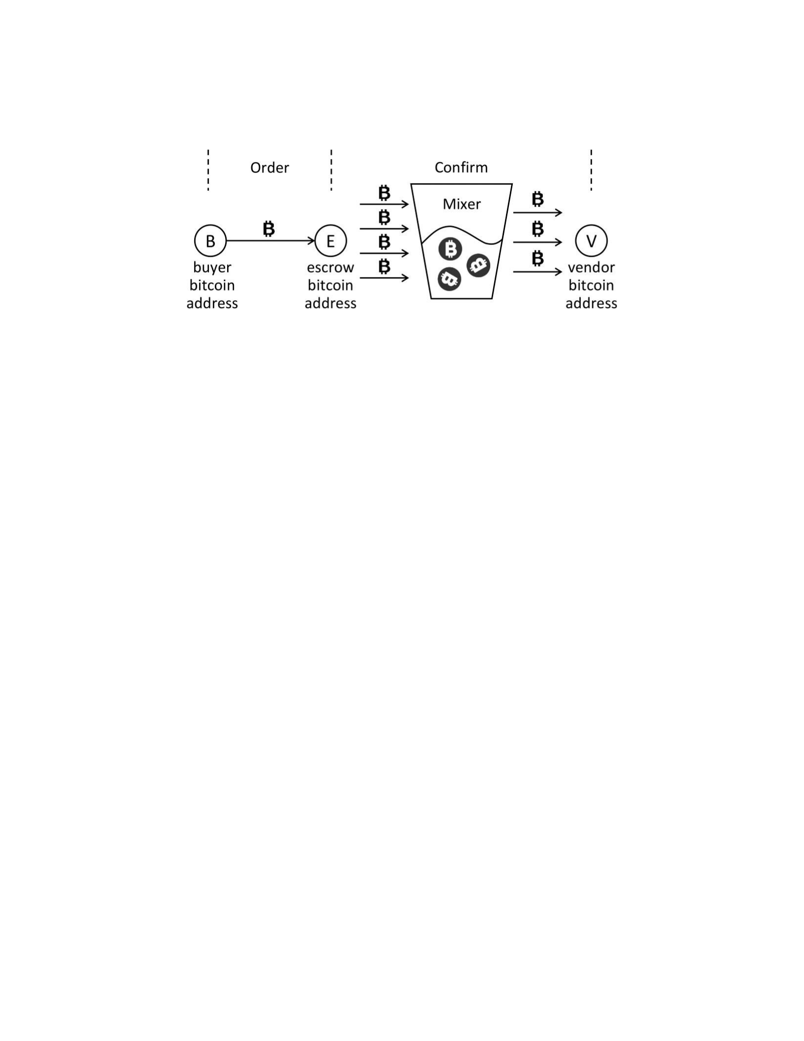
the vendor’s address through a mixed transaction. Mixed transactions are utilized to break

the

Figure (3.1) Bitcoin Flow of One Purchase in Wall Street Market

direct connection between the sender and receiver address by combining several

transactions into one transaction with multiple senders and multiple receivers [30,31].

However, we still can get the amount of Bitcoin received by each receiver address in mixed

transaction.

In Wall Street Market, 94.5% of Bitcoin in escrow address is sent to the vendor’s address,

and the remaining 5.5% is transferred to the Wall Street market address as a commission fee

during a mixed transaction. When the buyer confirms that they have received the illicit

product, they need to write feedback that appears in the review list of products with time

and amount of dollars spent during this transaction. Experiments we have in Wall Street

Market show the time when the review posted is close to the time when a mixed transaction

happened and the price of a product should be close to the Bitcoin value received by the

vendor’s address. Each feedback review is matched to a Bitcoin transaction based on

timestamp and value transferred in this transaction. If we could find the related Bitcoin

transaction in the public ledger, the receiver of this transaction is the Bitcoin address from

the vendor.

3.2 Related Work

3.2.1 Bitcoin De-anonymization

The rise of Bitcoin has increased researchers’ interest in privacy provided in

cryptocurrency [32–36], also the usage of Bitcoin in darknet [37]. To attack the privacy of

Bitcoin, the most common way is to study the Bitcoin transaction graph after clustering the

Bitcoin address from one wallet. A wallet represents an entity. A user stores all addresses in

a wallet. Researchers have widely clustered Bitcoin addresses heuristically. Androulaki

tested the effectiveness of the Bitcoin address clustering methods with simulation [34].

Spagnuolo links the clustered addresses to the Silk Road escrow address exposed by the FBI

and analyzes the Bitcoin flow related to this escrow address [32]. Fleder not only linked the

clustered addresses to Silk Road escrow but also linked Bitcoin addresses to some public

entities [33]. PageRank is then applied on the transaction graph to find addresses that are

close to the Silk Road escrow address. In the transaction graph, each node represents an

entity that contains all addresses owned by this entity. However, current clustering methods

don’t work for mixed transactions that combine several transactions into one transaction

with multiple senders and multiple receivers. Mix is quite common in Bitcoin transactions,

especially illegal transactions in recent years. In this chapter, our method is the first one to

explore relationships between feedback of vendors and receiver parts of Bitcoin transactions

which won’t be affected by mixed transactions.

3.2.2 Matching

If we treat each review as one type of node and Bitcoin transaction as another type of

node, reviews of a vendor and transactions from an address can form a bipartite graph after

we link the review to the matched transaction. Portnoff matches specific ads to publicly

available Bitcoin transactions based on the cost of ads and timestamp at which the ad was

placed [38]. Hungarian algorithm and Hopcroft-Karp algorithm are two greedy algorithms

that can successfully find the maximum matching in bipartite graph [39–41]. We can use

these algorithms to find the maximum matching between a vendor and a Bitcoin address.

However, this method is not effective enough to match multiple addresses. A vendor in the

darknet normally owns a lot of Bitcoin addresses.

3.2.3 Submodular Function

Submodular optimization algorithm has been exploited in other areas before [42–45].

Kempe using a greedy algorithm based on submodular function to maximize the influence in

Table (3.1) Main Symbols

symbols

definitions

b(t,u,r)

a Bitcoin transaction with timestamp t, money value u, and

receiving address r

a set of Bitcoin transactions, B = {bi(ti,ui,ri)}

R = {ri}

f(τ,v)

t v

F = {fj(τj,vj)}

S(R)

a set function, input R: a set of receiving Bitcoin addresses, output:

the set of feedback reviews matched with R

s(R)

a set function, input R: a set of receiving Bitcoin addresses, output:

the number of feedback reviews matched with R, i.e., s(R) = |S(R)|,

where | · | represents the cardinality of a set

social networks [46]. Leskovec exploits the submodularity of outbreak detection to develop

an efficient approximation algorithm for water distribution and the blogosphere monitoring

problem [47].

3.3 Problem Formulation

In this section, we formulate the problem of matching Bitcoin transactions with feedback

reviews. Table 3.1 shows the main symbols used in this chapter and their definitions.

Let B = (b1(t1,u1,r1),b2(t2,u2,r2),···,bn(tn,un,rn)) represents the set of all Bitcoin

transactions, where bi(ti,ui,ri) represents a Bitcoin transaction with three attributes:

timestamp ti, money value ui, and receiving address ri. Here we only need receiver part of

these

Bitcoin transactions. Let R represent a set of all unique receiving addresses in B. Let F =

(f1(τ1,v1),f2(τ2,v2),···,fm(τm,vm)) represents a list of feedback reviews received by one vendor,

where fj(τj,vj) is a feedback review with two attributes: timestamp τj and money value vj.

Vendor Receiving Address Set Problem:Finding a set of receiving addresses Rk ⊂ R

which are likely the Bitcoin addresses in the vendor’s wallet, according to the matching

between the vendor’s feedback reviews in set F and Bitcoin transactions in set B.

Based on practical observations, the timestamp τj and money value vj in fj(τj,vj) Table (3.2)

An Example to Illustrate the Vendor Receiving Address Set Problem

Input

After matching

all Bitcoin

feedback

Bitcoin

receiving

transactions B

reviews F

transactions

addresses

b1(t1,u1,r2)

f1(τ1,v1)

b1(t1,u1,r2)

r2 r3

r4 r5

b2(t2,u2,r3)

f2(τ2,v2)

b2(t2,u2,r3)

b3(t3,u3,r4)

f3(τ3,v3)

b3(t3,u3,r4)

b4(t4,u4,r5)

f4(τ4,v4)

b4(t4,u4,r5)

b5(t5,u5,r6)

f5(τ5,v5)

b5(t5,u5,r6)

b6(t6,u6,r1)

f6(τ6,v6)

f2(τ2,v2)

b6(t6,u6,r1)

r1 r7

b7(t7,u7,r7)

f7(τ7,v7)

b7(t7,u7,r7)

b8(t8,u8,r1)

f3(τ3,v3)

b8(t8,u8,r1)

r1 r8

b9(t9,u9,r8)

b10(t10,u10,r1)

f4(τ4,v4)

b10(t10,u10,r1)

r1 r2

r3 r4

b11(t11,u11,r2)

b12(t12,u12,r3)

b13(t13,u13,r4)

b14(t14,u14,r9)

b15(t15,u15,r1)

f5(τ5,v5)

b15(t15,u15,r1)

r1 r3

b16(t16,u16,r3)

b17(t17,u17,r5)

b18(t18,u18,r1)

f6(τ6,v6)

b18(t18,u18,r1)

r1 r3

b19(t19,u19,r3)

b20(t20,u20,r2)

f7(τ7,v7)

b20(t20,u20,r2)

r10

b21(t21,u21,r10)

···

are approximately equal to the timestamp ti and money value ui in a Bitcoin transaction

bi(ti,ui,ri) respectively, i.e., τj ≈ ti and uj ≈ vi, if bi(ti,ui,ri) is the corresponding Bitcoin transaction

of the feedback review fj(τj,vj). By comparing the timestamp and money value attributes, we

can match feedback reviews to Bitcoin transactions thus finding the receiving addresses. In

case the vendor does not change the receiving addresses frequently, many of their feedback

reviews will be matched with Bitcoin transactions with the same receiving addresses.

Problem 3.3 aims at finding a set of receiving addresses Rk ⊂ R whose involved Bitcoin

transactions match the maximum number of feedback reviews in F.

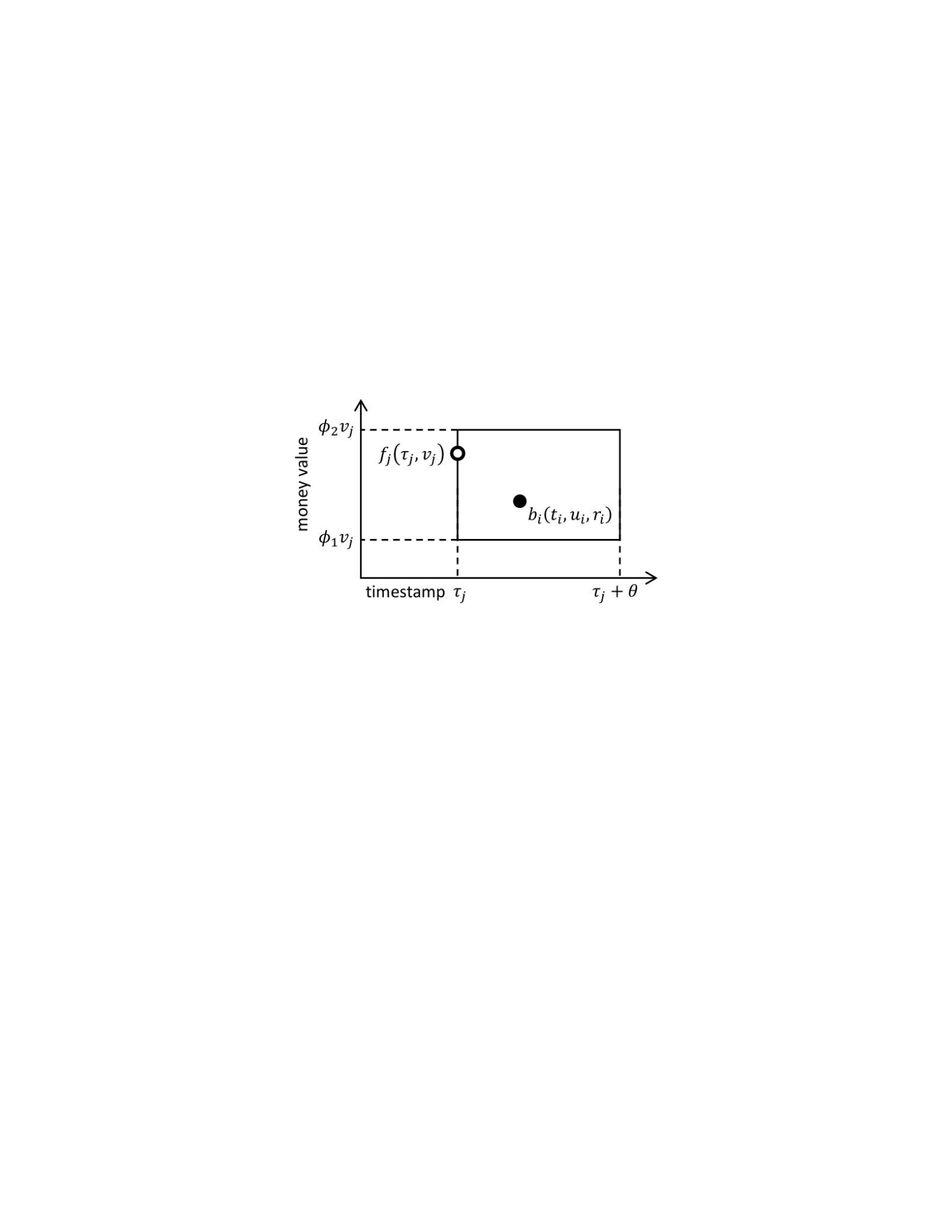
We use a bounding box to find candidate Bitcoin transactions for a feedback review. For

each review, we search the Bitcoin transactions B with a bounding box. We set thresholds θ

and φ to constrict the ranges of timestamp and money value respectively. Currently, there

Figure (3.2) Bounding Boxes of Timestamp and Money Value for Matching a Feedback Review

with a Bitcoin Transaction

are thousands of Bitcoin transactions every second. We compare a feedback review with a

Bitcoin transaction and we are able to match a review to thousands of candidate transactions

in real data with the range we provided. According to research [29], a Bitcoin transaction

happens within an hour after a buyer posts the review with a high possibility. Therefore, we

use τj ≤ ti ≤ τj + θ as the bounding box for timestamp and set θ = 1 hour. The market takes

5.5% commission fee and the exchange rate also fluctuates in a day. Therefore, we use φ1vj ≤

ui ≤ φ2vj as the bounding box for money value. If the fluctuation range is 10%, the setting will

be φ1 = (1 − 5.5%)(1 − 10%) = 0.8505 and φ2 = (1 − 5.5%)(1 + 10%) = 1.0395. Figure 3.2

illustrates the bounding boxes. If a Bitcoin transaction bi(ti,ui,ri) falls in the bounding boxes

of a feedback review fj(τj,vj), we say bi and fj are a match, which is formally defined in

Definition 3.3.

fj is matched with bi : A feedback review fj(τj,vj) is matched with a Bitcoin transaction

bi(ti,ui,ri) if τj ≤ ti ≤ τj + θ and φ1vj ≤ ui ≤ φ2vj.

Table 5.2 shows an example. The left part of Table 5.2 shows the input set B of Bitcoin

transactions and the input set F of feedback reviews received by a vendor. Because of the

limited space, only 21 Bitcoin transactions are shown here but B should contain hundreds of

millions of transactions. In the example, the vendor has 7 feedback reviews. The right part of

Table 5.2 shows the matches between the 7 feedback reviews and the 21 Bitcoin Table (3.3)

Vertical and Binary Format

receiving Bitcoin

feedback reviews

support

binary format

address ri

S({ri}) matched with ri

s({ri})

representation

f2,f3,f4,f5,f6

0, 1, 1, 1, 1, 1, 0

f1,f4,f7

1, 0, 0, 1, 0, 0, 1

f1,f4,f5,f6

1, 0, 0, 1, 1, 1, 0

f1,f4

1, 0, 0, 1, 0, 0, 0

f1,f5

1, 0, 0, 0, 1, 0, 0

1, 0, 0, 0, 0, 0, 0

0, 1, 0, 0, 0, 0, 0

0, 0, 1, 0, 0, 0, 0

0, 0, 0, 1, 0, 0, 0

r10

0, 0, 0, 0, 0, 0, 1

transactions. To save space, we ignore the concrete values of timestamps and money values

in B and F in the left part. Whenever there is a match, it means that the feedback review and

Bitcoin transaction satisfy Definition 3.3. From the right part of 5.2, we can see that there

could be multiple Bitcoin transactions that are matches of one feedback review. In real cases,

a feedback review could match hundreds of Bitcoin transactions. And the receiving addresses

in those matched Bitcoin transactions are the candidate addresses of the vendor.

In order to accelerate the computation in the later stages, we transfer the matching

results to the vertical and binary formats in Table 3.3. To solve Problem 3.3, we aim at finding

a minimum set of Bitcoin addresses covering all feedback reviews. The intuition is that a

Bitcoin address that can cover many feedback reviews is very likely to belong to the vendor

wallet. This is especially true when the careless vendor infrequently or barely changes their

Bitcoin address.

Let S(R) represents a set function which returns the set of feedback reviews that are

matched with the input set R of Bitcoin addresses. Let s(R) represent a set function which

returns the number of feedback reviews matched with the input set R, i.e., s(R) = |S(R)|.

Theorem 3.3 shows that s(R) is a submodular set function [46].

Given three Bitcoin address sets A, B, C with A ⊆ B ⊆ C and a Bitcoin address

r ∈ C \ B, we have

s(A ∪ {r}) − s(A) ≥ s(B ∪ {r}) − s(B) (3.1)

The left equation s(A∪{r})−s(A) represents the number of feedback reviews that are newly

matched after adding the Bitcoin address r to the set A. Thus, we have s(A∪{r})−s(A) = s({r})

− |S(A) ∩ S({r})|. Similarly, s(B ∪ {r}) − s(B) = s({r}) − |S(B) ∩ S({r})|. Since A ⊆ B, A are

matched with less or equal feedback reviews than B, i.e., S(A) ⊆ S(B), we have S(A) ∩ S({r}) ⊆

S(B) ∩ S({r}) thus |S(A) ∩ S({r})| ≤ |S(B) ∩ S({r})|. Therefore, s({r}) − |S(A) ∩ S({r})| ≥ s({r}) −

|S(B) ∩ S({r})|. This completes the proof.

Theorem 3.3 exhibits the diminishing returns property, which is the equivalent

condition of a submodular set function. The property can be explained as that the marginal

gain from adding a Bitcoin address to the set R is at least as high as the marginal gain from

adding the Bitcoin address to a superset of R. We aim at finding a receiving address set R with

size k, i.e., |R| = k, which can maximize s(R).

We decompose Problem 3.3 into two steps, which are formulated as Problem 3.3 and

Problem 3.3. Problem 3.3 aims at matching Bitcoin transactions with feedback reviews.

Problem 3.3 aims at searching the optimal set of Bitcoin addresses for a vendor. The output

of Problem 3.3 is the input of Problem 3.3.

Bounding Box Matching Problem: Given the set of Bitcoin transactions B, the set of

feedback reviews F, and the bounding box parameters θ for timestamp, φ1 and φ2 for money

values, the problem aims at finding a family of sets {Si}, where Si represents the set of feedback

reviews covered by candidate receiving address ri.

Maximum Review Coverage Problem: Given a family of sets {Si} with Si representing

the set of feedback reviews matched with each ri in bi(ti,ui,ri) ∈ B and a positive integer k as

the budget for the number of receiving addresses, the problem is finding an address set R

with size k, i.e., |R| = k, that are matched with the maximum number of feedback reviews.

That is, finding the optimal solution R of the following optimization problem:

max s(R)

s.t. |R| = k

Problem 3.3 can be solved in polynomial time.

Problem 3.3 is NP-hard. Problem 3.3 can be reduced from the famous Set Cover problem

[48]. Let X = {X1,··· ,Xq} be a family of sets with being the

elements. The NP-complete Set Cover problem aims at finding whether there exist k of the

subsets in {Xi} whose union is equal to Y . Given an arbitrary instance of the Set Cover

problem, we define a corresponding instance of Problem 3.3. For each subset Xi ∈ X, we create

a Bitcoin address ri and a set Si. Therefore, we get a family of sets {Si} and Rall = {r1,··· ,rq},

where all ri’s are unique. For each element yj, we create a feedback review fj. Therefore, we

get F = {f1,··· ,fp}. We add fj to Si, i.e., ri is matched with fj, if and only if Xi contains yj. The Set

Cover problem is equivalent to deciding if there is a set R ⊆ Rall of k Bitcoin addresses with

s(R) = p.

3.4 Computing Algorithms

In this section, we discuss how to efficiently compute the problems. We first study the

bounding box and KD tree techniques for matching the Bitcoin transactions with feedback

reviews. We then exploit a greedy algorithm that can obtain an address set that is provably

cover (1 − 1/e) ratio reviews of optimal. Here e is Euler’s number. Finally, we propose our fast

method which can accelerate the whole process by effectively reducing the times of matching.

3.4.1 Bounding Box and K-D tree

For each pair of feedback review f ∈ F and Bitcoin transaction b ∈ B, we need to check

the inequalities of timestamp and Bitcoin value. Let n = |B| be the number of Bitcoin

transactions in B and m = |F| be the number of feedback reviews in F. It runs in O(mn) to

compare reviews with all Bitcoin transactions.

Algorithm 4: Build KD Tree(B, η, d) [49]

Input: Bitcoin transaction set B, max depth η, current depth d Output: a

KD-tree T

if d < η then // d < η, a non-leaf node of the KD-tree create a KD-tree T with a root node π;

if d is odd then // d is odd, split by the timestamp

π.t ← the median value of all timestamps in B; split B

into B1(t < π.t) and B2(t ≥ π.t) by time;

else // d is even, split by the money value

π.u ← the median value of all money values in B; split B

into B1(u < π.u) and B2(u ≥ π.u) by value;

Tleft ← BuildKDTree(B1,η,d + 1); // build the left KD-tree Tright ←

BuildKDTree(B2,η,d + 1); // build the right KD-tree add a left child

sub-tree Tleft and a right child sub-tree Tright to π;

else // d = η, a leaf node of the KD-tree create a KD-tree T with a single node π containing set

To speed up the search process, we build a 2-D tree for the Bitcoin transaction set B

where the 2 dimensions are timestamp and money value. The reason that we build a KD-tree

for B, not for F is that the number n of Bitcoin transactions is generally much larger than the

number m of feedback reviews of a vendor. Algorithm 4 shows a recursive method for

building a KD-tree with a fixed height η from set B. In the even depth nodes of the KD-tree,

timestamp is used for partitioning the Bitcoin transactions. In the odd depth nodes of the KD-

tree, money value is used. To build the entire KD-tree, we call “BuildKDTree(B, η, d = 1)” in

algorithm 4 and pass the entire set B, the maximum depth η of the KD-tree, and the initial

depth d = 1 to the function. Figure 3.3(a) shows an example of building a KD-tree and Figure

3.3(b) shows the resulting KD-tree. In each depth d, Algorithm 4 needs a linear time O(n) to

find the median and split the set into left and right subsets. Algorithm 4 runs in O(ηn).

Algorithm 5 shows the improved bounding box search algorithm using the KD-tree. For

each feedback review f, Algorithm 5 will find the leaf nodes in the KD-tree that may contain

Bitcoin transactions matched with f. Searching a KD tree runs in O(2η) in the worst case. W

represents all leaf nodes of the KD-tree that are returned. In general, the number of returned

leaf nodes is small. Suppose on average, the number of returned leaf nodes is

(a) coordinate system representation (b) tree representation

Figure (3.3) K-D Tree and Range Searching

Algorithm 5: Bounding Box Search with KD Tree(B, T, F, η, θ, φ1, φ2)

Input: Bitcoin transaction set B, KD-tree T built from B, feedback review set F, max depth η,

bounding box parameter θ for timestamp, φ1 and φ2 for money value

Output: a family of sets {Si}, where Si represents the set of feedback reviews matched with ri in

bi(ti,ui,ri) ∈ B

for each unique ri in bi(ti,ui,ri) ∈ B do Si ← ∅; // initialization fj(τj,vj) ∈ F : W =

KDTreeSearch(root node of KD-tree T, f(τ,v), η, θ, φ1, φ2); bi(ti,ui,ri) ∈ W : if τj ≤ ti ≤ τj

+ θ and φ1vj ≤ ui ≤ φ2vj then

γ. Since there are 2η leaf nodes, there are O(n/2η) Bitcoin transactions in each leaf node.

Therefore, Algorithm 5 runs in O((γ +η)mn/2η) on average. It is much faster than O(mn).

γ is small in our experiments on real data.

←

∪{

}

;

3.4.2 Greedy Set Cover Algorithm

Algorithm 6 shows a greedy algorithm with a ratio (1 − 1/e) of optimal for solving

Problem 3.3. In Algorithm 6, we start with an empty address set R0 = ∅, and add a Bitcoin

address ri in each iteration which maximally increases the review coverage s(Ri).

Algorithm 6 has an approximation ratio of (1 − 1/e). That is, s(Rk) ≥ (1 − 1/e)s(A∗) where

A∗ represents the k-size address set which matches maximum reviews and k is the size of

returned address set.

The proof can be found in [50]. The key observation is that s(R) is non-decreasing

submodular set function according to Theorem 3.3.

Algorithm 6: Greedy Set Cover Algorithm({Si}, λ)

Input: a family of sets {Si}, where Si represents the set of feedback reviews matched with ri in

bi(ti,ui,ri) ∈ B, a threshold λ ∈ (0,1) Output: optimal number k

r1 ← argmaxr∈R s(r); R1 ← {r1};i ← 1; // extract the best matching

(s(Ri) − s(Ri−1))/(s(Ri−1) − s(Ri−2)) < λ ri+1 ← argmaxr∈R\Ri(s(Ri ∪ {r}) − s(Ri)); Ri+1 ← Ri ∪ {ri+1},

i + +; return Ri−1;

Algorithm 7: Cost-Effective Addresses Searching(B, F, θ, φ1, φ2, λ)

Input: Bitcoin transaction set B, feedback review set F, bounding box parameter θ for

timestamp, φ1 and φ2 for money value, a threshold λ ∈ (0,1) Output: a set Rk of Bitcoin

addresses belonging to a vendor

R0 ← ∅; F0 ← ∅; α0 ← None; // Stage 1: an address with max coverage s(α0) < |F \

F0| Fα0 ← all feedback reviews matched with Bitcoin address α0; f ← select a

feedback review from F \ (F0 ∪ Fα0) at random; R0 ← R0 ∪ { Bitcoin addresses

matched with f}; F0 ← F0 ∪ {f}; α0 ← argmaxr∈R0 s(r); // extract the best

matching address

R1 ← {α0}; i ← 1; // Stage 2: searching for a set of addresses

(s(Ri) − s(Ri−1))/(s(Ri−1) − s(Ri−2)) > λ Fα0 ← all feedback reviews matched with Bitcoin address α0;

F ← F \ Fα0;F0 ← F0 \ (F0 ∩ Fα0);

α0 ← argmaxr∈R0 s(r); // best matching address based on new F Ri+1

← Ri ∪ {α0}; i + +; return Ri−1;

Algorithm 6 can decide the number of addresses to return with a threshold λ. Intuitively

a vendor’s Bitcoin addresses should match many more of their feedback reviews compared

with noise Bitcoin addresses that do not belong to them. This phenomenon is also proved in

our experiments on real-life data. We calculate the ratio of increments in review coverage in

two consecutive iterations. If the ratio is less than a threshold λ ∈ (0,1), the greedy algorithm

will terminate and output address set.

3.4.3 Cost-Effective Addresses Searching

Algorithm 5 will find matched Bitcoin transactions for all feedback reviews in F. And the

following greedy algorithm 6 will find an optimal address which cover most reviews

iteratively. The whole process is time consuming. In this section, we propose a CostEffective

Addresses Searching(CEAS) algorithm which will find the optimal address with much less

matching calculations between reviews and Bitcoin transactions. The steps are shown in

algorithm 7. In CEAS, we only needs to apply range searching for (|F|−s(rmax)+1) reviews,

where rmax is the address that covers maximum reviews. Therefore s(rmax) is the maximum

number of reviews matched by a single address. Experiments show that CEAS can prunes

about 60% comparisons between reviews and Bitcoin transactions.

Let F represents full feedback reviews and F 0 represents feedback reviews set which we

have already applied range searching for. R is the address set containing all addresses and R0

represents address set containing addresses matched by any reviews in F 0. We have

following theorem.

Let α = argmaxr∈R s(r) and α0 = argmaxr∈R0 s(r). If s(α0) ≥ |F \ F 0|, we have α0 = α. α is the

address in R that matches the maximum number of reviews and α0 is the address in R0 that

matches the maximum number of reviews. For any Bitcoin address r ∈ R \ R0, it doesn’t match

any reviews in F 0. Therefore, the maximum number of reviews that r can match is |F \ F 0|. If

s(α0)|F \ F 0|, address α0 matches more reviews than any address r ∈R \R0, which makes α0

the address that matches largest number of reviews in set R. This completes the proof.

According to Theorem 3.4.3, we can find the optimal address in R0 which is also the

optimal address we could find in R when the condition s(α0) ≥ |F \ F 0| is satisfied. Therefore

we don’t need to apply range searching in KD-tree for all reviews in R to get this optimal

address.

In all addresses R, to find the optimal address which matches maximum number of

reviews in F, The number of feedback reviews |F 0| we need to apply range searching for is

bounded as |F| − s(rmax) ≤ |F 0| ≤ |F| − s(rmax) + 1.

rmax represents the address in R that matches maximum reviews. s(rmax) represents the

number of feedback reviews that are matched with the address rmax. To satisfy the condition

s(α0)|F \ F 0| in theorem 3.4.3, we have |F 0| ≥ |F|−s(α0) ≥ |F|−s(α) = |F|−s(rmax). At the same

time, α need to match at least one review in F 0, which requires at most (|F|−s(rmax)+1) times

of range searching.

Now we know we need at most (|F| − s(rmax) + 1) times of range searching to get the

optimal address. In greedy algorithm, we need to repeat this step for k times to obtain the

optimal k-size address set. We can prove that finding the optimal address set still need at

most (|F| − s(rmax) + 1) times range searching.

To find optimal address set in greedy Algorithm 7, the total number of feedback reviews

|F 0| we need to apply range searching is still bounded as |F|−s(rmax) ≤ |F 0| ≤ |F|−s(rmax)+ 1.

After we apply |F| − s(rmax) or |F| − s(rmax) + 1 times of range searching to get the first address.

The next address should be the one which matches maximum reviews in the remaining

reviews based on greedy algorithm. We can remove reviews covered by the first address and

use the same method to find the second address which matches maximum reviews in the

remaining reviews. When we select feedback review to apply range searching in step 4 of

algorithm 7, we avoid the reviews which are matched with address α0. As a result, in all |F| −

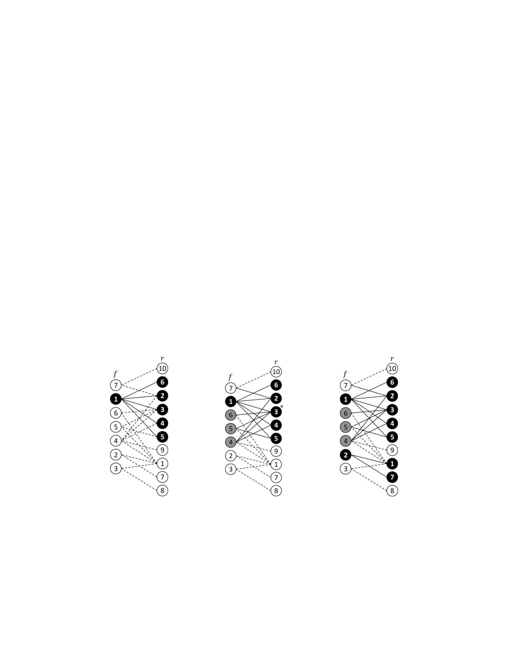
s(rmax) feedback reviews where we apply range searching on, only one feedback review match

with the address rmax. After we remove reviews covered by the address rmax. In the remaining

F − s(rmax) reviews, there should be |F| − s(rmax) − 1 reviews that have already gone through

range searching. Now we can update F = (F − s(rmax)) and update F 0 = (|F|−s(rmax)−1). Then

the new |F \ F 0| = ((F −s(rmax))−(|F|−s(rmax)−1) = 1, which means s(α0) ≥ |F \ F 0| in theorem

3.4.3 is always satisfied. Therefore we don’t need to apply range searching to any more

reviews to find remaining addresses of vendor.

Figure 3.4 explains CEAS Algorithm using the example in Table 5.2. In Figure 3.4, we use

a bipartite graph to represent the matches between feedback reviews and receiver addresses.

Each node on the left represents a feedback review and each node on the right represents a

receiver address. An edge represents that a feedback review is covered by this address. A

dotted edge represents a non-computed match and a solid edge represents a computed

match. We re-order the nodes on both sides to reduce the visual clutter.

In Stage 1, Algorithm 7 randomly selects f1 in line 4 and finds its matched Bitcoin

addresses {r2,r3,r4,r5,r6} in line 5. Now F 0 = {f1} and R0 = {r2,r3,r4,r5,r6}. We use black

(a) after line 4, 5 (b) after line 6, 3 (c) after line 4, 5

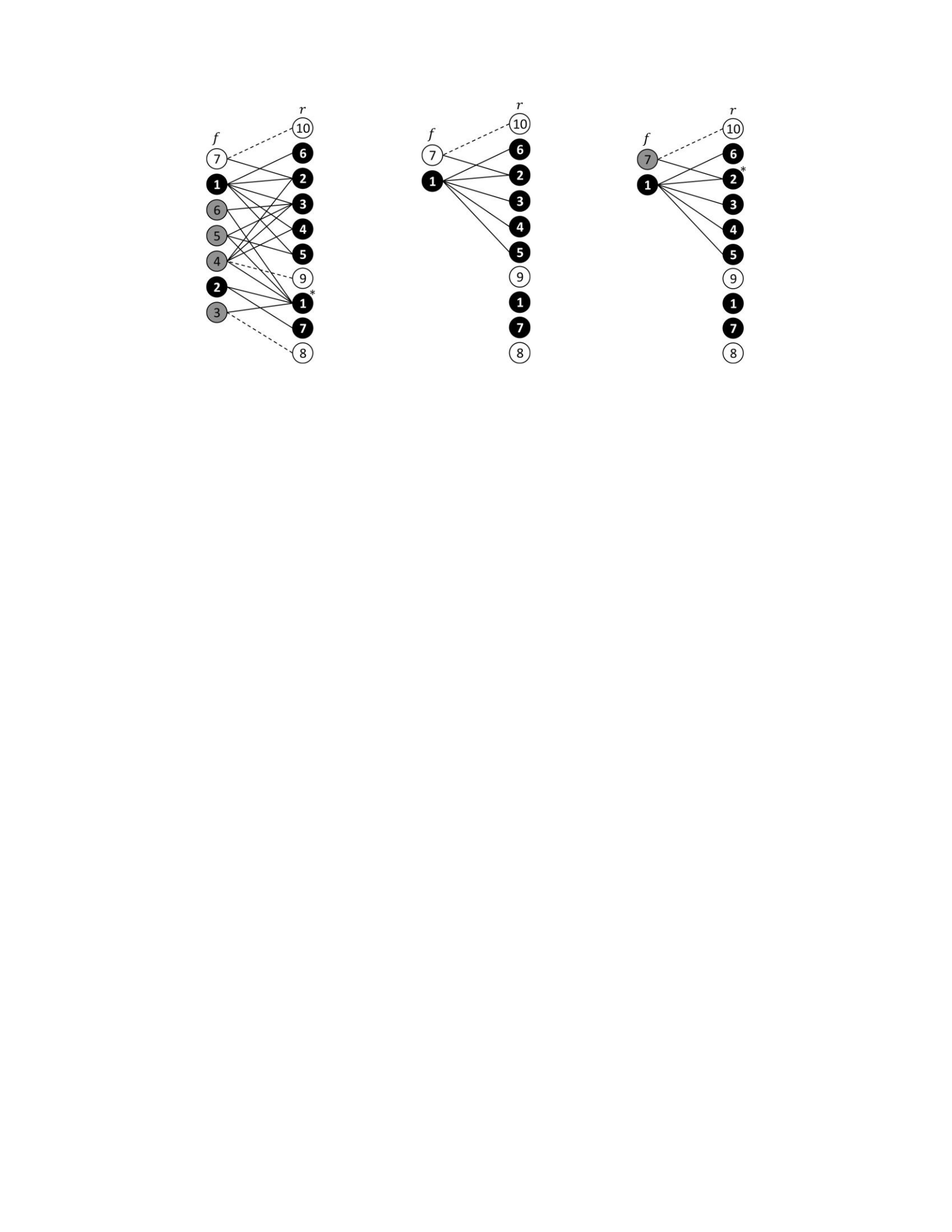
(d) after line 6 (e) after line 10 (f) after line 11

Figure (3.4) An Example for the Heuristic Search in Algorithm 7 (F: nodes on the left; F 0:

black nodes on the left; R0: black nodes on the right; the “line” refers to the lines in Algorithm

nodes to represent them in Figure 3.4(a). Algorithm 7 extracts the Bitcoin address r3 from R0

since it has the largest number of matched feedback reviews. In Figure 3.4(b), we use “∗” to

represent the Bitcoin address in R0 with the maximum coverage. Now Fα0 = {f1,f4,f5,f6}.

Algorithm 7 then randomly selects f2 from the review set F \(F 0 ∪Fα0) = {f2,f3,f7} in line 4 and

finds its matched Bitcoin addresses {r1,r7} in line 5. Now R0= {r1,r2,r3,r4,r5,r6,r7} and F 0 = {f1,f2}.

Figure 3.4(c) shows the status. Algorithm 7 extracts the Bitcoin address r1 from R0 since it has

the largest number of matched feedback reviews, which is shown in

Figure 3.4(d). Since s(rmax) = s({r1}) = 5 ≥ |F \ F 0| = 5, Stage 1 is done.

In Stage 2, Algorithm 7 first adds the best Bitcoin address r1 into the resulting set thus

rmax = r1. Since r1 is matched with Fr1 = {f2,f3,f4,f5,f6}, Algorithm 7 deletes the reviews covered

by r1 from the left part and the associated edges. Figure 3.4(e) shows the remaining graph.

Now F = {f1,f7} and F 0 = {f1}. Algorithm 7 then selects the best matching address from R0 based

on the new F = {f1,f7}. Since r2 has the largest number of matches thus is optimal. Algorithm 7

will terminate in the next iteration since all feedback reviews have been covered and the drop

is larger than λ.

Here we only need to search matched Bitcoin transactions for f1 and f2. This is one

possible solution for this example. In algorithm 7, we randomly select review to apply range

searching. No matter how we select reviews, it always needs to apply range searching for 2

or 3 reviews in this example, which is the range of |F 0|. In this example,2 ≤ |F 0| ≤ 3 because

s(rmax) = 5 and |F| = 7. In contrast, Algorithm 5 need apply range searching for all 7 feedback

reviews. According to Theorem 3.4.3, Algorithm 7 always finds the same best Bitcoin address

that Algorithm 6 finds.

Time Complexity: Line 5 in Algorithm 7 performs the bounding box search and is the

most time consuming step and dominates the time complexity. This is because the number

of Bitcoin transactions n is much larger than other parameters like m. Based on Theorem

3.4.3, the times of running line 5 is upper bounded by |F 0| ≤ m−s(rmax)+1. Thus Algorithm 7

runs in O((γ + η)(m − s(rmax) + 1)n/2η). Please refer to last paragraph in Section 3.4.1 for more

details.

3.5 Experimental Results

In this section, we conduct extensive experiments to evaluate the efficiency and

effectiveness of our method by using both real and synthetic datasets. All algorithms are

implemented in Python and all the experiments are conducted on a Linux Server with Intel

Xeon 3.2GHz CPU and 32 GB main memory.

Datasets. For the real dataset, we crawled feedback from Wall Street Market. Wall

Street Market sells a variety of content, including drugs, stolen data, and counterfeit

consumer goods, all using cryptocurrency. In the Wall Street market, each vendor has a list

of reviews. Each feedback contains the time when the buyer leaves this feedback as well as

the amount of Bitcoin used in this transaction. Here we crawled the feedback of different

vendors and sum the transactions to a file, one transaction was represented by a 2-

dimensional data (τ,v), where τ is the timestamp when this review was posted and v is money

cost in this purchase. Here, we collect transactions of different vendors in Dec 2018. There

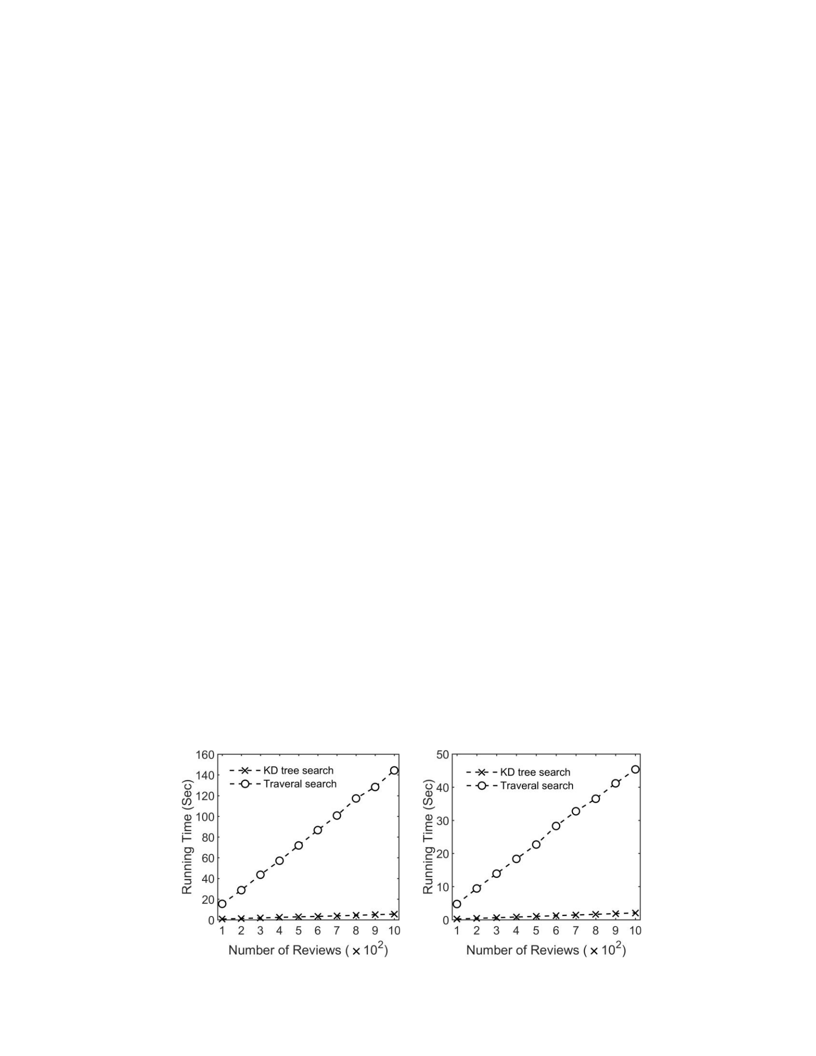
are in total 17,155,754 Bitcoin transactions during this time. The synthetic dataset is

produced by the Bitcoin transaction data.

Next, we first evaluate the efficiency of K-D tree and greedy algorithm by real dataset

and then the accuracy by synthetic dataset.

3.5.1 Efficiency Evaluation in Range Searching

Each review we have can generate a 2-dimensional range based on the Bitcoin value and

timestamp. With this range, we search the Bitcoin public ledger to find a lot of candidate

transactions matched to this review. Figure 3.5 demonstrates that the K-D tree we build can

effectively save time during range searching. We build a K-D tree with the real dataset,

separating transactions into 16,384 buckets with a 14-depth binary tree. Each bucket

contains more than one thousand transactions. We sample reviews from Wall Street Market.

Bitcoin transactions are divided through Bitcoin value and timestamp alternately. Figure

3.5(a) shows the comparison of time-consuming in K-D tree and traversal in full ledger. It

only takes less than 5.5 seconds to find the matched transactions for 1000 reviews in the K-

D tree, nearly 5.5 milliseconds for one review. We also built another K-D Tree with a smaller

data size, including only mixed transactions in Bitcoin public ledger. Users in cryptomarkets

prefer mixed transactions to protect their privacy in Bitcoin transactions. We conduct the

same experiment in this filter ledger which contains 1,395,694 Bitcoin transactions. Figure

3.5(b) shows the result with K-D tree structure; it only takes around 2 milliseconds to find

the matched transactions for a review.

(a) range searching in full ledger (b) range searching in filtered ledger

Figure (3.5) Compare Running Time of K-D Tree Searching and Traversal Searching in Full

Ledger and Filter

3.5.2 Effectiveness Evaluation of Greedy Algorithm

Our greedy algorithm guarantees that we can achieve at least (1 − 1/e) of maximum

coverage theoretically. Here we speed up our greedy algorithm by removing low degree

addresses found in range searching and evaluate the performance of the greedy algorithm on

the real dataset.

We select feedback from 100 vendors with 3721 reviews. Matched Bitcoin transactions

of reviews from a vendor can be found through the K-D tree, which helps us get matched

addresses of each review. By changing this data format to vertical format like Table 3.3, we

get the reviews covered by each matched address for a vendor. Now we are looking for a

receiver address set whose transactions can match the maximum reviews. Based on the range

we set, a review can normally be matched to thousands of transactions in the Bitcoin ledger.

Only one of these matched addresses can be the vendor’s address, which means the

remaining addresses are noises in our algorithm. In the experiments, 94.23% of the

addresses we found only match one review. 5.26% of addresses match 2 reviews and only

0.51% addresses match more than 2 reviews on average. Heuristically we are looking for

addresses that can match the maximum reviews. Therefore, removing addresses with a low

degree will not affect the accuracy of our algorithm. We conduct the simple greedy

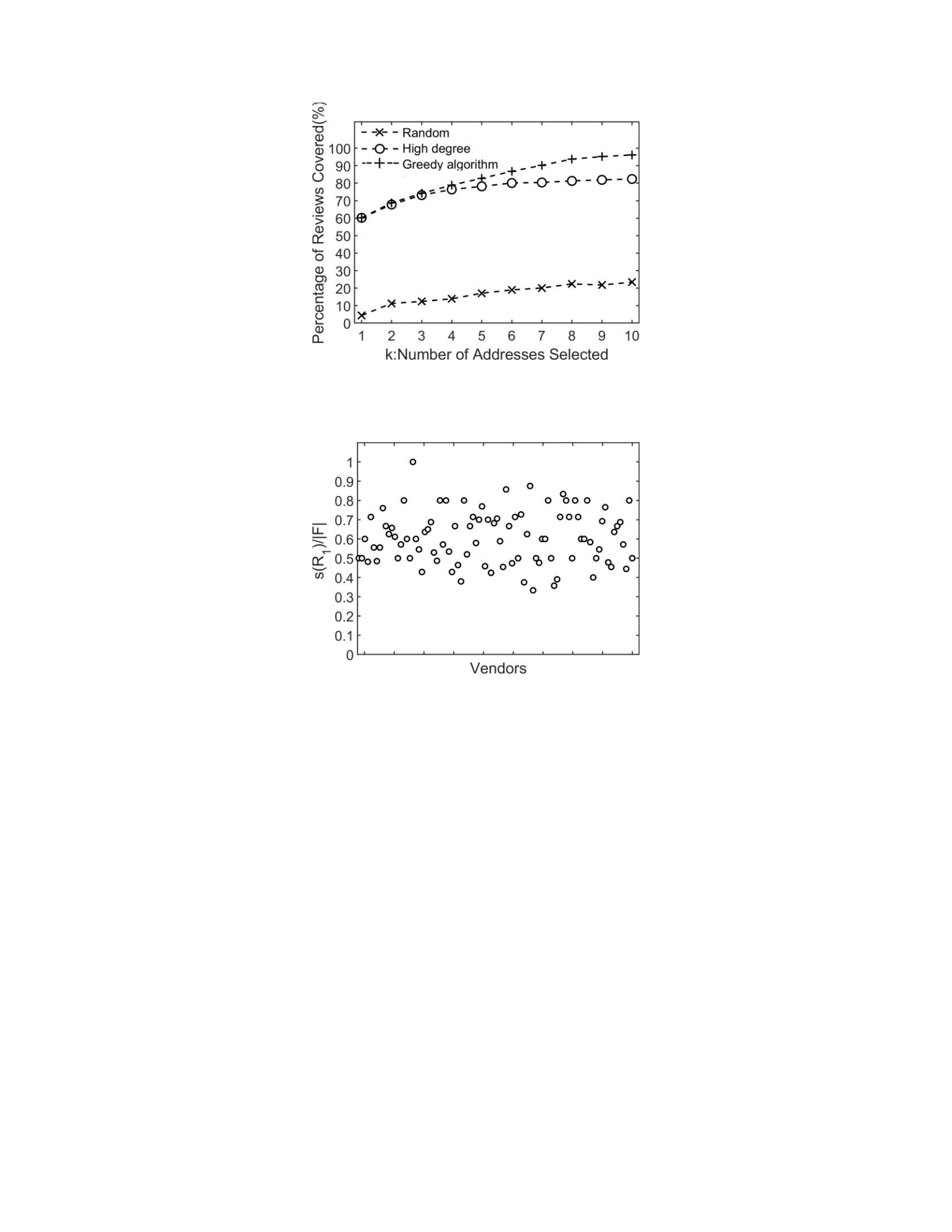
Figure (3.6) Greedy Agorithm Outperform High Degree and Random Method

Figure (3.7) Maximum Reviews Covered by One Address in Ratio for Different Vendors

algorithm without setting a threshold λ. We set k from 1 to 10 as the number of output

addresses. The greedy algorithm needs to output an address set that covers as many reviews

as possible. Result demonstrates that we can save 93% time if we ignore address matching

with only 1 review during the greedy algorithm and 99% time if we remove addresses with

a degree less than 3.

To evaluate the performance in the maximum coverage of the greedy algorithm. We

compare the greedy algorithm with a heuristic high degree method and the random selection

method. The high degree method will select addresses with the maximum review coverage.

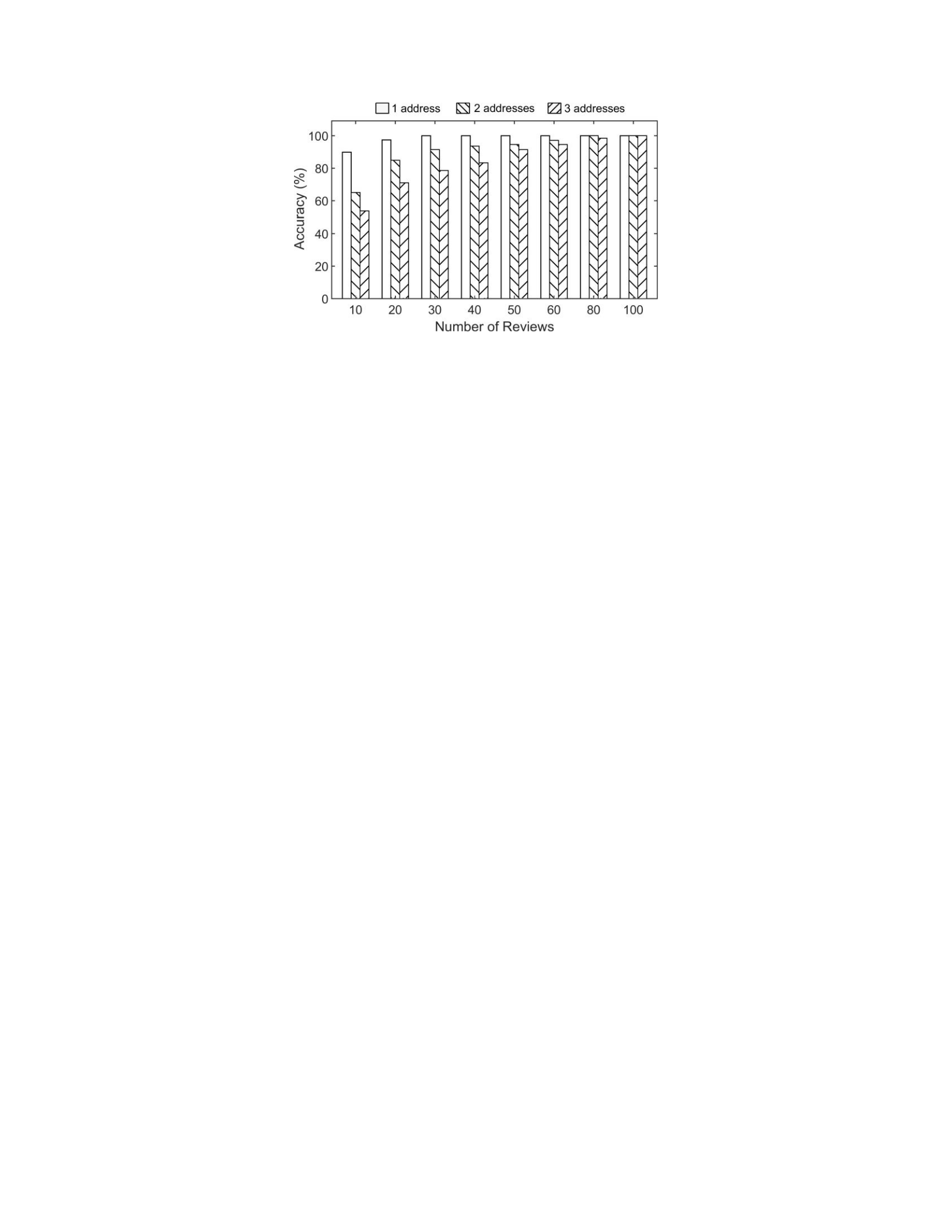
Figure (3.8) Accuracy Comparison Between Vendors with Different Number of Addresses

We average the percentages of reviews covered. From Figure 3.6, we can notice that the

performance of the high degree method is similar to the greedy algorithm when k is small. As

k increases, the gap between these two methods increases.

The number of times in range searching is at most |F| − s(R1) + 1 in our proposed

algorithm. We can reduce at least s(R1) − 1 times. s(R1) is the number of reviews covered by

the first address we get in the greedy algorithm, which also is the address rmax that covers

maximum reviews in F. The more reviews covered by this address, the fewer times of range

searching are required. Figure 3.7 shows the ratio s(R1)/F of 100 vendors we find in Wall

Street Market. Each node in Figure 3.7 represents a vendor. We can see that the address which

covers the maximum reviews can cover between 35% to 90% of all reviews from a vendor

and 60.217% on average, which means we can reduce times of range searching by 60.217%.

We find 66% of these vendors whose reviews can be matched to an address that covers more

than half of the reviews. The result shows the effectiveness of our algorithm in the real

dataset and unveils that the vendors in Wall Street Market do not change their receiving

addresses frequently.

3.5.3 Accuracy Evaluation on Synthetic Data

In this section, we conduct experiments to evaluate the accuracy of our algorithm on

synthetic reviews. We select 2000 Bitcoin addresses and collect their history transactions.

Each transaction contains timestamp and Bitcoin value received, which can be treated as a

review after a slight change. We apply normal distribution on the amount of change in both

Bitcoin value and timestamp. The number of hours we advance on timestamp follows the

normal distribution with 0.5 mean and 0.6 std. In probability, the newly generated review’s

bounding box in timestamp will cover the transaction at 59% feasibility. The same strategy

is applied to the Bitcoin value. After combining the restrict of timestamp and Bitcoin value,

the newly generated review can match to the original transaction with a 35.4% possibility.

Every address we randomly select from the Bitcoin ledger can generate a synthetic review

list. Considering vendors may use multiple Bitcoin addresses, we also combine some

synthetic reviews generated by different addresses.

Figure 3.8 shows the accuracy of the greedy algorithm with reviews generated by 1

address, 2 addresses, and 3 addresses. Accuracy is the number of correct addresses over the

number of addresses that generate these synthetic reviews. From Figure 3.8, we can see that

longer review lists contribute to better accuracy, while more receiver addresses can reduce

accuracy, which matches the real situation. It is hard to find the vendor’s address set if the

vendor updates their receiver address in the darknet market very frequently. For vendors

who do not change their receiver address frequently, our algorithm can achieve great

performance even with very few reviews.

We set a threshold λ for the ratio of new reviews covered in the current step to new

reviews covered in the last step. We use synthetic data generated by different numbers of

addresses to evaluate the effect of different λ. For reviews generated from one address, Figure

3.9 shows larger λ has better performance because we do not want to select another address

besides the one with the highest degree. Reviews derived from 2 or more addresses share a

similar pattern. Large λ can decrease the accuracy because a high threshold will stop the

greedy algorithm too early and output fewer addresses than the vendor have. The more

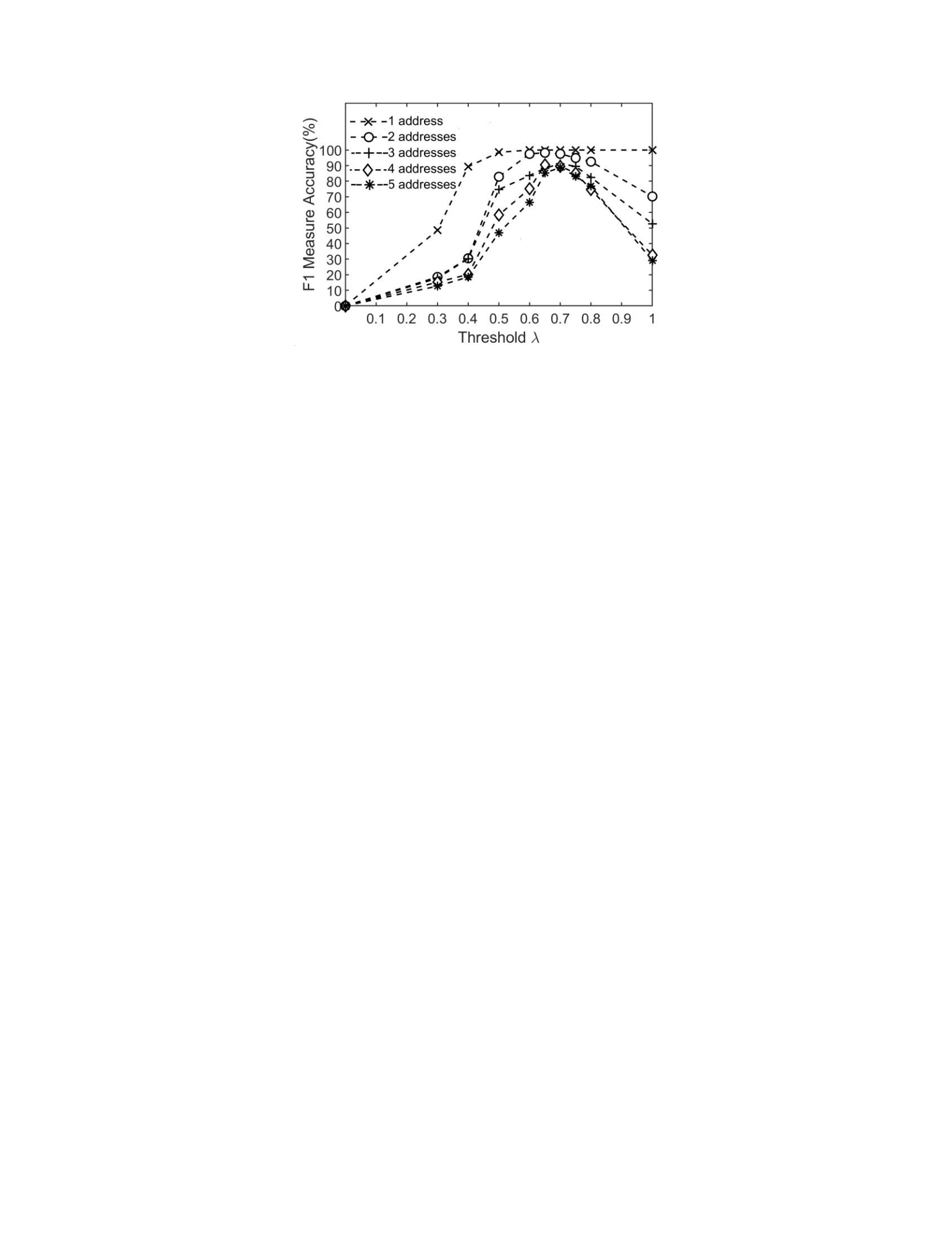
Figure (3.9) F1 Measure Accuracy of Synthetic Data Generated from Different Number of

Addresses

addresses a feedback related, the fast the drop of accuracy after λ pass 0.7. Through the

experiments, we can see λ around 0.7 is the best option for all these data.

3.6 Conclusion

In this chapter, we study the problem of identifying the Bitcoin addresses of a vendor by

matching their feedback reviews with Bitcoin transactions. We firstly construct a KD tree to

efficiently match Bitcoin transactions to feedback reviews. After we obtain the matching

relationship between Bitcoin transactions and feedback reviews, we get the address set by

applying a greedy algorithm that can achieve a near-optimal theoretical guarantee. We

further develop a Cost-Effective Address Searching(CEAS) algorithm that can speed up the

process by pruning the search space effectively. Comprehensive experiments on both real and

synthetic datasets demonstrate the effectiveness and efficiency of our methods.

PART 4

LEARNING INFECTIVITY GRAPH IN CHAT GROUP VIA

TEMPORAL-TEXTUAL MULTI-DIMENSIONAL HAWKES PROCESS

In this chapter, we propose an effective model to discover hidden infectivity networks

between members in a group chat.

4.1 Motivation

Telegram, as one of the most popular instant message applications, becomes the base for

criminal activities. For example, the ”Nth Room” case. The ”Nth Room” case is a criminal case

involving blackmail, cybersex trafficking, and the spread of sexually exploitative videos via

the Telegram app between 2018 and 2020 in South Korea. The channel ”Nth Room” in

Telegram is where criminals communicate and commit activities. Telegram also has many

public chat channels with illegal content. We can search the name of darknet market in

Telegram. All these darknet markets manage a public chat channel in Telegram and we can

easily find these chat channels and join them. Learning Granger causality for members in a

chat group is meaningful for law enforcement. The Granger causality among members helps

us to construct an influence network, which is beneficial to discover organizations behind

these criminal activities and the related key person.

Unfortunately, identifying influence between members in a public group chat is not a

simple task when there are thousands of members. Analyzing from a large amount of chat

conversations could be challenging and time-consuming. Existing works about group chat

mainly focus on community detection or topic detection. Farkhund applies data mining and

natural language processing techniques on chat log[51,52]. They proposed a framework

which extracts the social network from chat logs and summarizes conversation into topics.

Anwar presents a unified social graph based text mining framework to identify digital

evidences from chat logs data[53], which considers both users’ conversation and interaction

data in group chats to discover overlapping users’ interests and their social ties. However,

these researches didn’t investigate directional impact between members.

4.2 Related Work

We perform a literature review focusing on following two aspects: 1) Problems about

multiparticipant chat analysis and how these have been addressed. 2) Hawkes processes for

their dominant usages in self- exciting or mutual-exciting event sequence learning

subsectionMultiparticipant Chat Communications through instant message applications

have remained under a substantial study over the last few years. Due to increasing popularity,

both structural and textual content of chat data are being investigated in various

perspectives. Researchers have mainly focused on problems including preprocessing of text

data[54–56], conversations disentanglement [57–60], topic detection[51,52,61] and

community detection in chat logs[51–53,62,63].

There is a lot of overlap between chat preprocessing techniques and those used in other

forms of microtext— normalizing the unusual, informal text characteristics. Each has

described an expanded taxonomy of semiotic classes for text[54]. Sproat and Jaitly present a

recurrent neural net (RNN) model of text normalization[56], where they model text

normalization as a sequence-to-sequence problem. Chua et al. describes an automated

multilanguage text normalization infrastructure that prepares textual data to train language

models used in Google’s keyboards and speech recognition systems, across hundreds of

language

varieties[55].

A common phenomenon in group chats is that multiple conversations are mixed

together. In group chat, a newly sent message may not be the response of the latest message

when multiple conversations occur simultaneously. Therefore thread disentanglement is one

of the major task in group chat analysis. In [57], Elsner proposes a graph-theoretic model for

disentanglement, using discourse-based features which have not been previously applied to

thread disentanglement. Focusing on NLP techniques on real dataset, Kauttonen analyzed

two conversational corpora: A public library question-answering (QA) data and a private

medical chat data they developed response retrieval (ranking) models using TF-IDF,

StarSpace, ESIM and BERT methods [60]. For researchers who want to learn their thread

disentanglement models with annotated datasets, Kummerfeld et al. released a new dataset

of 77,563 messages manually annotated with reply-structure graphs that both disentangle

conversations and define internal conversation structure[58].

Topic detection and community detection is high level analysis in group chat analysis.

Many efforts have been made to extract key topics and network from large chat logs. In

[51,52], Iqbal first discovers the communities based on the co-occurrence frequencies of the

entities in chat sessions, further they mine corresponding concepts by identifying important

terms based on their frequency in the text. Anwar presents a unified social graph based text

mining framework to identify digital evidence from chat logs data[53]. To study the

characteristics of chat messages, Dong et al. analyzes a collection of 33,121 sample messages

gathered from 1,700 sessions of conversations and concludes indicative term-based

approach is superior to the traditional document frequency based approach, for feature

selection in chat topic categorization[61]. In this chapter, we work with Hawkes process

model to extract mutual influence factors, instead of detecting communities directly.

4.2.1 Hawkes Process

Hawkes processes [64] have been widely used to model time-series events where the

occurrences of previous events could trigger the occurrences of future events. Those models

successfully discover the influence network among events and predict future time-

dependent event sequences. Researchers link triggering kernels of Hawkes process to

granger causality of different event types successfully[65–70]. It has been utilized in areas

including earthquake shocks prediction[71,72], financial markets analysis [73,74], health

analysis[69,75] and criminal activities[70,74].

Several teams have achieved remarkable results in Hawkes process for mutual-exciting

event sequence learning. Zhou et al. focuses on the nonparametric learning of the triggering

kernels in Hawkes process[67], proposing an approach to discover the hidden network of

social influence in sparse low-rank networks[66]. Linderman develops a probabilistic model

that combines Hawkes processes with random graph models and discovers the latent

network of stock trading, gangs activities and calcium imaging[74,76]. Through an infinite

order autoregression, Eichler designs a new nonparameteric estimator of the impact

functions of the Hawkes process[65]. They apply this model to neural spike train data and

study the mutual-exciting networks of spinal dorsal horn neurons under different conditions.

Xu et al. represents the kernel functions with a series of basis functions and extract the

influence graph through group sparsity of the kernel functions’ coefficients.[68].

Howkes process can also be modeled to predict time series data. Xu et al. develops a

novel framework based on Hawkes process to predict patient flow[69]. His team further

model incomplete sequence data with Hawkes process by leveraging the idea of data

synthesis[77]. They also discuss an effective model-based clustering method based on a novel

Dirichlet mixture model of Hawkes process[78].

Most of the kernel functions of Hawkes process in existing works are decaying functions

like power-law functions or exponential functions based on time. In this chapter we embed

the text information from group chat into the kernel function of Hawkes process to describe

a more precise influence network.

4.3 Proposed Model

As time series data, the chat history of a group can be considered as event sequence set

C = {S1,S2,...}, where sequence Sk represents a segment of chat in a chat group. Every Sk =

(m1k,m2k,...) is a sequence of message mik = (tik,dik,xik) where tik is time when the message was

sent, dik is the member identity who sent this message and xik is the text

content.

To uncover the latent infectivity network in group chat, our method contains two steps.

dialogue Classifier: For a message mj in group chat, to find which message it replied to, we

embed each pair of messages (mi,mj) to a number eij ∈ {0,1} based on semantics in text from

mi and mj. Here eij classify whether that message mj replies to mi semantically. Text biased

Marked Multi-dimensional Hawkes Process: We model the chat history with a multi-

dimensional hawkes process. In this model, message sequences in chat history are event

sequences and the sender of the message is marked as the type of this event. We train this

model based on observed chat history with learned dialogue classifiers.

4.3.1 Dialogue Classifier

In group chat, we want to get the relationship between the current message and previous

messages semantically. They could be irrelevant or the current message is the response to

one or several previous messages.

In this chapter, we pretrain text pairs with a BERT model, followed by a classifier. BERT

is designed to pretrain deep bidirectional representations from text by jointly conditioning

on both left and right context in all layers[79]. It’s empirically powerful and has obtained

state-of-art results on several natural language processing tasks. We input two texts to Bert

pretained model which converts text pairs to a vector. This vector is further input to a

downstream task classifier to fine-tune the pretrained Bert model. The classifier will classify

whether the second text is a reply to the first text or not semantically. The output of the last

layer should be a number e ∈ {0,1}. Here e = 0 means it is not a reply and e = 1 represents it

is. We can use this output number as the measure of the second text replying to the first text.

For message mi, the message it replies to should be close with message mi in time. In

group chat, members normally wouldn’t reply to a message a long time ago. Therefore, it’s

not necessary to calculate reply embedding of each pair of messages and only consider

message pairs Within a limited time frame.

4.3.2 Temporal-Textual Multi-dimensional Hawkes Process

Although hawkes process can model time series sequence, there are two limitations of

the one-dimensional hawkes process for our problem. One is that it can only model a single

type of event. If we want to capture the interacting processes between members in a chat

group, message sequences from different members should be treated as different types of

events. Another limitation is that triggering the kernel only decays with time difference.

Reply embedding of message pairs can also help us quantify the influence of a past event on

the new event. If two messages are not classified as a conversation, we are supposed to know

the previous message will not trigger the later message. Therefore we need a multi-

dimensional hawkes process including reply embedding.

In our problems, message sequences in chat history are event sequences that we try to

model. Sender d of the message could be marked as the type of this message.

Multidimensional hawkes process can capture the mutual excitations among different types

of events. Instead of using α to represent influence strength from previous events, we have

matrix A = [αij] capturing the mutual influence in a group. Given event sequences

((t1,d1),(t2,d2),...), the intensity function of type d at time t is

λd(t) = µd + X αdjd · g(t − tj) (4.1)

j:tj<t

where µd is exogenous base intensity of event type d. Here it means base activity level

of user d in this group chat. The second term on the right side are influence from previous

messages. αdjd is the strength of influence from person dj on person d in this group.

If the new message is not a reply to a previous message, this new message is not

triggered by this previous message. To leverage text information between current message

mi(ti,di,xi) and a previous message mj(tj,dj,xj), we update trigger kernel from g(ti − tj) to g(ti −

tj) · h(xj,xi), where h(xj,xi) ∈ {0,1} is the reply embedding. Give chat history

((t1,d1,x1),(t2,d2,x2),...), the intensity function of member d at time t with text x is

λd(t,x) = µd + X αdjd · g(t − tj) · h(xj,x) (4.2)

j:tj<t

Here we utilize the reply embedding h(xj,x) to filter the influence from previous messages.

Only messages responded by a new message have influence on the occurrence of this new

message.

4.3.3 Learning Task

To find the infectivity matrix A = [αij], we need to derive the likelihood function of this

hawkes model. Suppose we have a chat history H = ((t1,d1,x1),(t2,d2,x2),...(tn,dn,xn)), Let F(t|H)

be the conditional probability that next message (tn+1,dn+1,xn+1) appears before time t, where

t > tn. We have F(t|H) = P(tn+1 < t). And let p(t|H) be the corresponding conditional probability

density function. Then we have expected instantaneous happening rate of message λ(t) =

p(t|H)/(1−F(t|H)), from where we can get the conditional probability density function for a

specific member d with text x as

(4.3)

Here is the probability that the next message appears after time t based on

given history H. λd(t,x) is the intensity function of user d at time t sending text x.

Let event sequence represents chat history we observed in t ∈ [0,T],

we can derive the likelihood function of observed sequence as:

Y −RtTN λ(τ)dτ

pdi(ti,xi|Hi)e (4.4)

i=1

where Hi is the history events before time ti.

Put intensity function into equation(4), the log-likelihood can be expressed as:

(4.5)

The learning problem is to find the matrix A = [αji] that maximizes log-likelihood

function L(A).

4.3.4 EM Algorithm

We need to find Matrix A = [aij] that maximizes log-likelihood function L(A). From

research [80], L(A) is concave. We can apply EM algorithm to solve this optimization problem

iteratively. In particular, we construct a tight lower-bound likelihood function for current

parameter estimation by Jensen’s inequality:

(4.6)

Here pii represents the probability that ith event occurred due to base intensity µdi. And

pji can be interpreted as the probability that the ith event is triggered by the jth event. We have

We can maximize our log likelihood by maximizing this lower bound. The EM algorithm

for the estimation of the parameters is as follows. Starting with a guess A = [αji] for the

parameters, iterate the following until convergence is reached:

Expectation-step:

(4.7)

(4.8)

Maximization-step:

(4.9)

(4.10)

Here u,v can represent any uses in group chat. It’s guaranteed that EM algorithm is able

to converge to the global maximum. We won’t show details here.

4.4 Experiments

In this section, we first compare the performance of bert-based language model with

XLNet-based language model in classification. we then conduct experiments using synthetic

group chat generated from different sources of dialogue and real world group chat from

telegram to fully evaluate the performance of our developed temporal-textual multi-

dimensional Hawkes model in infectivity Graph learning.

4.4.1 Dialogue Classifier Comparisons

Bert, as the state of art language representation model, is designed to pre-train deep

bidirectional representations from text by jointly conditioning on both left and right context

in all layers[79]. Before the emergence of Bert, existing approaches like ELMo and OpenAI

GPT use unidirectional language models to learn general language representations. Bert

alleviates the unidirectionality constraint by using a “masked language model” (MLM)

pretraining objective. Besides Bert, another state of art language representation model XLNet

also has the capability of modeling bidirectional contexts [81].

Here we compare the performance of the Bert-based model with the XLNet-based model

with the same size parameters. We train and test accuracy of the dialogue classifier based on

data we crawled from telegram group channels. In telegram, users are able to click the reply

button to reply to a specific utterance in group chat. Therefore a small part of utterance in

group chat explicitly shows which utterance it replies to and we are able to parse these

dialogue pairs of sentences. We can also select two random texts from group chat to create a

non-dialogue sentence pair.

Dialogue Datasets Besides chat logs from telegram, we train and test the performance

of dialogue classifiers with some public chitchat data as well. Here are the dialogue dataset

we used to train and evaluate our models.

• BSTalk BlendedSkillTalk is a dataset of 7k conversations explicitly designed to exhibit

multiple conversation modes: displaying personality, having empathy, and

demonstrating knowledge [82].

• ConvAI A dataset of Human-bot dialogues containing free discussions of randomly

chosen paragraphs from SQuAD.

• CMUDoG CMU Document Grounded Conversations is a document grounded dataset for

text conversations, where the documents are Wikipedia articles about popular movies.

Consists of 4112 conversations with an average of 21.43 turns per conversa-

tion[83].

• DSTC7 DSTC7 provides a dataset of dialogs that are derived from collections of

twoparty conversations. The conversations are randomly split part way through to

create a partial conversation and the true follow-up response.[84].

• PersonaChat(PC) A chit-chat dataset where paired Turkers are given assigned

personas and chat to try to get to know each other response.[85].

Table4.1 shows the data size of training data, which is the number of sentences pairs.

Table5.1 shows the classifier accuracy in different datasets. We can see the bert-based

language model outperform the XLNet-based model in all of these datasets.

Table (4.1) Data Size

Training Data

BSTalk

ConvAI

CMUDoG

DSTC7

Size

33368

104898

5602

38082

27882

48547

Table (4.2) Accuracy of Dialogue Classifiers

Model

BSTalk

ConvAI

CMUDoG

DSTC7

Bert-based

0.8044

0.9343

0.7068

0.7732

0.7881

0.8452

XLNet-based

0.7154

0.8692

0.5524

0.5031

0.6994

0.7525

4.4.2 Synthetic Data

The hard part of evaluation is that we can’t access the ground truth of the influence

network from public group chat logs. To illustrate that the proposed methods can precisely

extract the underlying influence network from observed chat sequences, we first conduct a

set of experiments in synthetic group chat generated from well-known dialogues data. We

applied Ogata’s thinning algorithm to simulate a multi-dimensional Hawkes process and get

the trigger of each event from previous events[86]. After we have timestamp and user for

each event in simulated Hawkes process, we further embed dialogues texts from some well-

known open source chitchat data to create synthetic group chat. In the simulated Hawkes

process, if a user d1 reply to user d2, the text embedded for d1 should be a replied text for d2’s

text in dialogue chitchat.

Here, we consider a n-dimensional Hawkes process. We random select n from 4 to 1000

for 100 times. We have n users in a group, d1,d2,d3 .... dn. In particular, we consider two

different types of influence matrix A in our experiments.

• Random Relationship For a random relationship case, we generate a matrix A where

αij is sampled randomly from [0,1] for i! = j. The exogenous base intensity of each user

is set to 0.01.

• Sub Group Relationship For sub group relationship case, we will assume there are

2 sub groups during n users. Users d1 to dn/2 are closely connected. User dn/2+1 to dn are

close friends as another sub group. We assign high value to influence inside each sub

group. We also assign low value to influence between users in different sub groups.

Here we will simulate 2 Hawkes Process at the same time with an influence matrix

A. These two Hawkes Process start with users from different groups. As a result, we

generate group chats where two conversations are mixed together.

Dialogue Datasets In generated data, we utilize some public dialogue datasets to create

conversations inside synthetic group chat. The datasets we applied in our experiments are

the same datasets we used to train the dialogue classifier, including BSTalk, ConvAI,

CMUDoG, DSTC7 and PersonaChat(PC).

Evaluation Metric We use two evaluation metrics to measure the performance:

• AveErr AveErr is defined as average error between real influence weight and the

extracted influence matrix.

• PearsonCor PearsonCor is defined as averaged Pearson correlation coefficient

between real influence matrix A and extracted influence matrix A0 , which meansures

the linear correlation between αij and α0ij

Models We extracted an influence matrix with four different models and compared the

results. Here are the methods we applied to

• TimeWindow(TW) We set a fixed length time window. An influence weight αij is

calculated based on the number of times user j speaks after user i within the fixed time

length.

• NR NR is the number of replies. Based on the reply embedding. A influence weight αij is

calculated based on the total reply embedding between user j and user i

• MHP MHP represents the Multi-dimensional Hawkes Process. This method will model

message sequences in a group chat to a multi-dimensional Hawkes process and learn

the Granger causality between different individuals by expectation-maximization

algorithm

• TTMHP TTMHP represents the Temporal-Textual Multi-dimensional Hawkes Process.

This is our proposed method in this paper which embed the text information of group

chat into the multi-dimensional Hawkes process

Table (4.3) Experiments Result

Matrix

Type

Method

BSTalk

ConvAI

CMUDog

DSTC7

AveErr

Random

MHP

TTMHP

0.942

0.988

0.407

0.399

0.964

0.959

0.369

0.368

0.977

0.956

0.511

0.486

0.947

0.936

0.443

0.352

0.965

0.932

0.492

0.422

Subgroup

MHP

0.866

0.890

0.625

0.859

0.919

0.610

0.857

0.930

0.576

0.842

0.922

0.631

0.845

0.899

0.625

TTMHP

0.289

0.425

0.295

0.326

0.384

PearsonCor

Random

MHP

TTMHP

0.697

0.769

0.734

0.867

0.546

0.704

0.761

0.947

0.488

0.583

0.616

0.940

0.665

0.787

0.745

0.861

0.558

0.692

0.713

0.938

Subgroup

MHP

0.584

0.980

0.366

0.577

0.851

0.147

0.522

0.891

0.430

0.549

0.955

0.291

0.529

0.841

0.216

TTMHP

0.996

0.947

0.966

0.952

0.943

Table 4.3 shows the average error and average Pearson correlation coefficient from our

experiments. From the result, we can see our proposed model, Temporal-Textual

Multidimensional Hawkes Process, achieves lowest error and highest correlation coefficient

with these five group chat logs generated by different types of dialogues.

For random relationship group chat, we can see Hawkes process model including MHP

and TTMHP get better results compared to Time window model and NR model. The time

window model can capture the influence based on timestamp. NR model is calculated based

on reply embedding. The performance of Hawkes process model implies that the Hawkes

Process can successfully extract the trigger pattern between utterances in group chat.

For the sub group relationship case, our proposed TTMHP model still achieves the best

result. Model NR is better than MHP in Pearson correlation coefficient. The reason is that

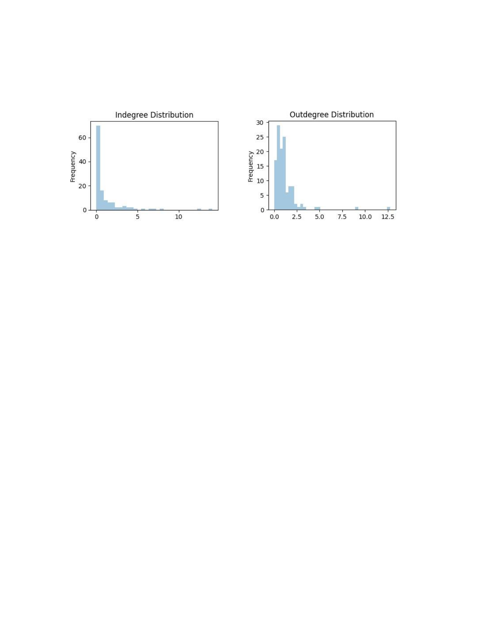
model NR can capture the text information in group chat. When the group chat data is a

combination of several sub groups, some close posts in a group chat could belong to different

topics. Models like NR and TTMHP that utilize text information can extract

(a) node in-degree distribution (b) node out-degree distribution

Figure (4.1) In-degree Distribution and Out-degree Distribution of an Telegram Group Chat

Channel

subgroup relationships better than models like Time window and MHP that only utilize time

difference.

4.4.3 Telegram Data and Case Study

To better understand the performance of the Temporal-Textual Multi-dimensional

Hawkes Process model on real data, we apply our proposed model to chat logs from telegram

group channels.

For the influence network we extracted, most members only interact with a few

members or don’t interact with others in the group. Figure 4.1 shows the influence’s in-

degree distribution and out-degree distribution of an example channel in telegram. We can

tell most people have low influence on others, which matches the reality that most people

don’t know each other in an online chat group.

Figure 4.2 shows an infectivity network of a 30 members group channel. In this graph,

each node represents a user in this group and a directed weighted edge represents the

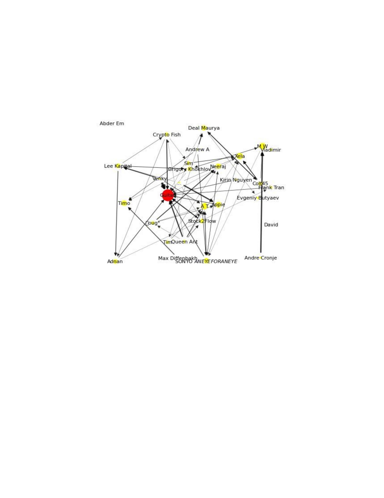
influence between users. To provide a more straightforward insight of the influence network,

we let the width of the edge proportional to influence coefficient and size of node

proportional to in-degree of influence. Here yellow nodes represent the normal members in

this group and the red node ”Guitar” represents the administrator of this group. From this

graph, node

Figure (4.2) Influence Network of an 80 Members Telegram Channel

”Guitar” has the maximum in-degree influence. By checking the chat history of this group, we

found that the user ”Guitar” answered a lot of questions and helped other members in this

group. This indicates the influence graph can reflect the trigger pattern of this group chat.

Such kind of information can provide investigative insight for law enforcement to analyze the

organization structure of members in these online groups.

4.5 Conclusion

In this paper, we study the problem of learning infecivity graph from group chat logs. We

firstly implement a dialogue classifier which can classify whether the second text is a reply

for the first text semantically when we input two sentences. We convert the group chat log to

an event sequence where every utterance is an event and the member who post this message

is the event type. We model the event sequence with multi-dimensional Hawkes process and

embed the text information we extracted through the dialogue classifier to kernal function of

the Hawkes process model. By applying an EM algorithm, we successfully extract the trigger

pattern between members inside a group channel. Comprehensive experimental results

show the effectiveness and efficiency of the proposed methods.

PART 5

CLUSTERING OF ACCOUNTS IN ONLINE MESSAGING SOFTWARE

THROUGH ATTRIBUTED HETEROGENEOUS INFORMATION

NETWORKS

In this part, we propose an effective model to learn the embedding of each account in

group chat. We further train a classifier to identify accounts that belong to the same user.

5.1 Motivation

The privacy of participants in illicit online transactions is protected through two parts.

One is the platform where vendors sell their products and the other is the emergence of

cryptocurrency.

Instant Message software like Telegram, providing public channels for users to discuss

and conduct illegal activities[9,53], become one of biggest platforms for illicit sales.

Telegram offers users a completely free open-source platform without any ads, a clean

interface, and (the biggest selling point) security[87]. One important feature of Telegram is

being able to search the channels posts, group messages, individual messages or any kind of

communications or posts. This feature is available for both cell phone applications and the

Web-based Telegram interface making it possible to reach any content by simply

searching[88,89]. This essentially makes Telegram one of the largest free databases available

to the public, especially considering the fact that many other media outlets, including Google,

Instagram, Twitter, and Facebook, are constantly removing illegal posts. Even though there

are illegal activities in these chat channels, administrators of these group channels still keep

these channels public to let new buyers and vendors join the channel easily. Users of

Telegram can search product names in Telegram and they are able to find related chat

channels easily without any effort. Figure 5.1 shows the result of searching the keyword

”silkroad” in

Figure (5.1) Searching SilkRoad in Telegram

Telegram. SilkRoad is one of the most famous darknets that sell drugs[90]. After joining these

channels, buyers can see the vendors posts about their products in the chat channel and

vendors can advertise their products periodically. If the buyer is interested in the product

posted by the vendor, he or she can discuss details with the vendor in the group channel or

create a private chat channel with the vendor.

To combat these illegal sales, it’s critical for law enforcement to know the organizations

of users in these group chat channels and analyze influence networks. However, no matter

vendors or buyers, they normally maintain multiple accounts in the Telegram platforms. To

track the ecosystem of users and build a network of the users, it’s critical that we are able to

link different accounts belonging to the same user.

Given the large number of users and millions of chat logs, it’s impossible to manually

label accounts of the same user and cluster them. Therefore, there is an urgent need to

develop a model which can automatically identify accounts belonging to one user or different

users.

The remainder of this paper is organized as follows. Section 2 review related work,

followed by the proposed methods in Section 3. Section 4 details our experiments. Section 5

shows case study and section 6 concludes the paper.

5.2 Related Work

We perform a literature review focusing on the following two aspects: 1) Study on

Telegram data 2) Time series data representation learning. 3) Graph Node representation

learning

5.2.1 Telegram

Telegram is an instant message application that can be accessed by a wide range of users.

To protect user’s privacy, Telegram provides encryption services for their customers, which

can prevent potential eavesdroppers – including software developers and internet providers.

However, these privacy-protecting and convenient software has been utilized by criminals

for illegal activities like drug smuggling, online fraudulence or even anti-social activities[9].

In recent years, a lot of works analyze the criminal activities data from Telegram[89,91–93].

Anglano presents a methodology for the forensic analysis of the artifacts generated on

Android smartphones by Telegram Messenger[91]. Their methodology is based on the design

of a set of experiments suitable to elicit the generation of artifacts and their retention on the

device storage. Satrya also presents a thorough description of all the artifacts that are

generated by the messenger application Telegram on Android OS[92]. Gregorio did similar

work for Windows phone, focusing particularly on how the information is structured and the

user, chat and conversation data generated by the application are organized, with the goal of

extracting related data from the information[93]. However, none of these works are trying to

identify different accounts that are managed by the same user.

5.2.2 Time Series Representation Learning

The aim of time series representation learning is to learn the embedding of time series

data that can be used to measure the similarity of two time series data. Learning universal

representations for time series is a fundamental but challenging problem.

Yue presents TS2Vec, a universal framework for learning representations of time series

in an arbitrary semantic level. Unlike existing methods, TS2Vec performs contrastive learning

in a hierarchical way over augmented context views, which enables a robust contextual

representation for each timestamp.[94]. Lei proposing an efficient representation learning

framework that is able to convert a set of time series with various lengths to an

instancefeature matrix. In particular, they guarantee that the pairwise similarities between

time series are well preserved after the transformation, thus the learned feature

representation is particularly suitable for the time series clustering task.[95] Eldele proposes

an unsupervised Time-Series representation learning framework via Temporal and

Contextual Contrasting (TS-TCC), to learn time-series representation from unlabeled

data[96]. These work measure similarity of two time series data with classic methods such

as Mikowski distance, crosscorrelation, Kullback-Leibler divergence, dynamic time

warping(DTW) similarity, movesplit-merge(MSM) distance, and short time series(STS)

distance. These researches focus on the time series data instead of timestamp. In our

problem, we want to know the similarity of two timestamp lists, which can’t be accurately

measured by methods like dynamic time warping. We develop a machine learning model that

can learn the representation of a time stamp list and measure the similarity between two

timestamp lists through learned embedding.

5.2.3 Graph Node Representation Learning

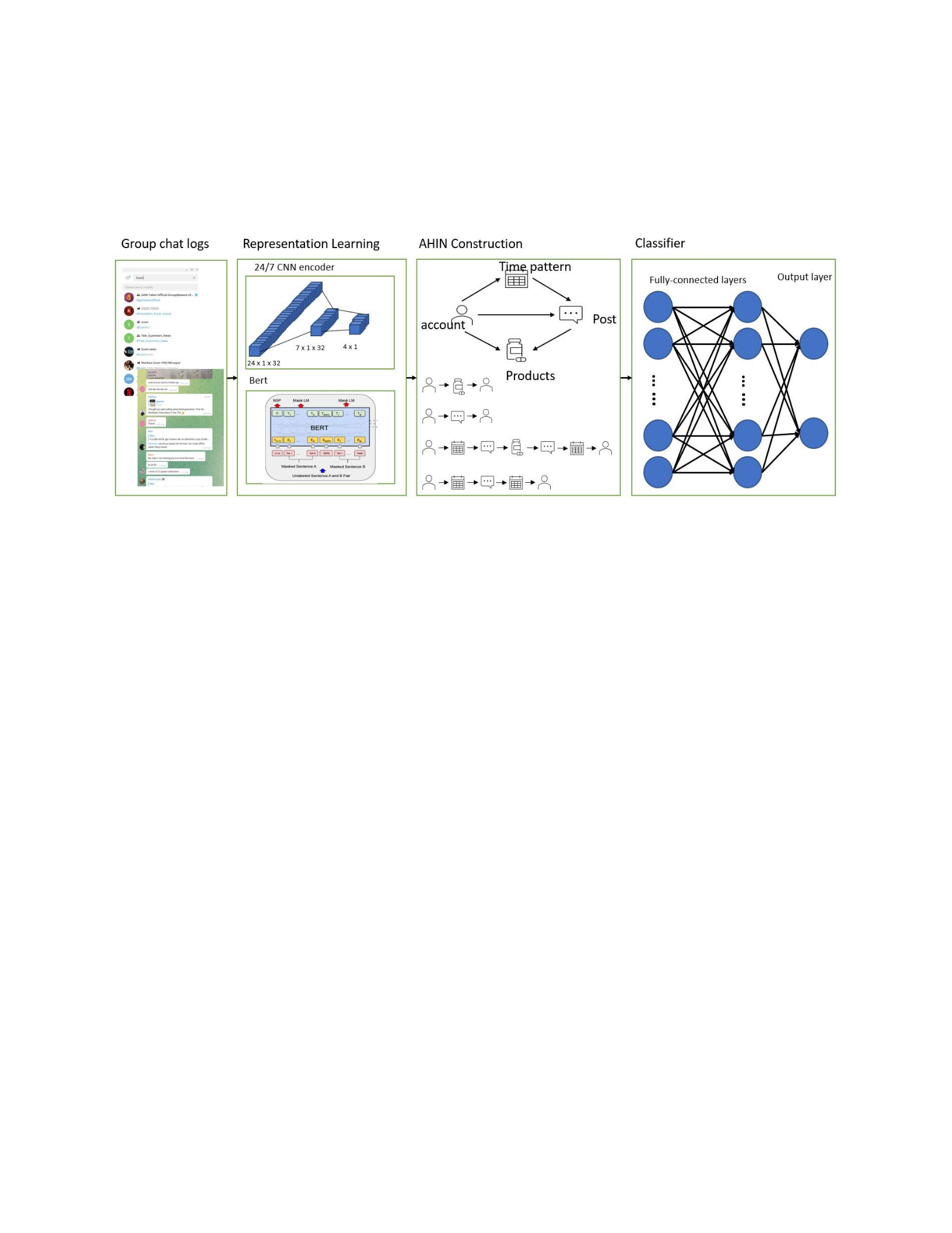
Since most real-world data can be conveniently represented by graphs, research on

graph representation learning has received increasing attention in recent years[97].

Classical graph embedding methods can be divided into linear and nonlinear categories.

Linear methods include: Principal component analysis (PCA)[98], Linear discriminant anal-

Figure (5.2) System Architecture

ysis (LDA)[99] and Multidimensional scaling (MDS)[100]. Non-linear dimensionality

reduction methods include: Isometric feature mapping (Isomap)[101], Locally linear

embedding (LLE)[102] and Kernel methods[103].

Random-walk-based methods sample a graph with a large number of paths by starting

walks from random initial nodes. DeepWalk learns these latent representations to encode

social relations in a continuous vector space. DeepWalk summarizes recent advances in

language modeling and unsupervised feature learning from word sequences to graphs[104].

node2vec is a modified version of DeepWalk, which defines a flexible notion of a node’s

network neighborhood and design a biased random walk procedure[105]. Our node

representation learning method utilizes the time pattern and text. We sample meta paths

from the AHIN we built and construct biased random walks.

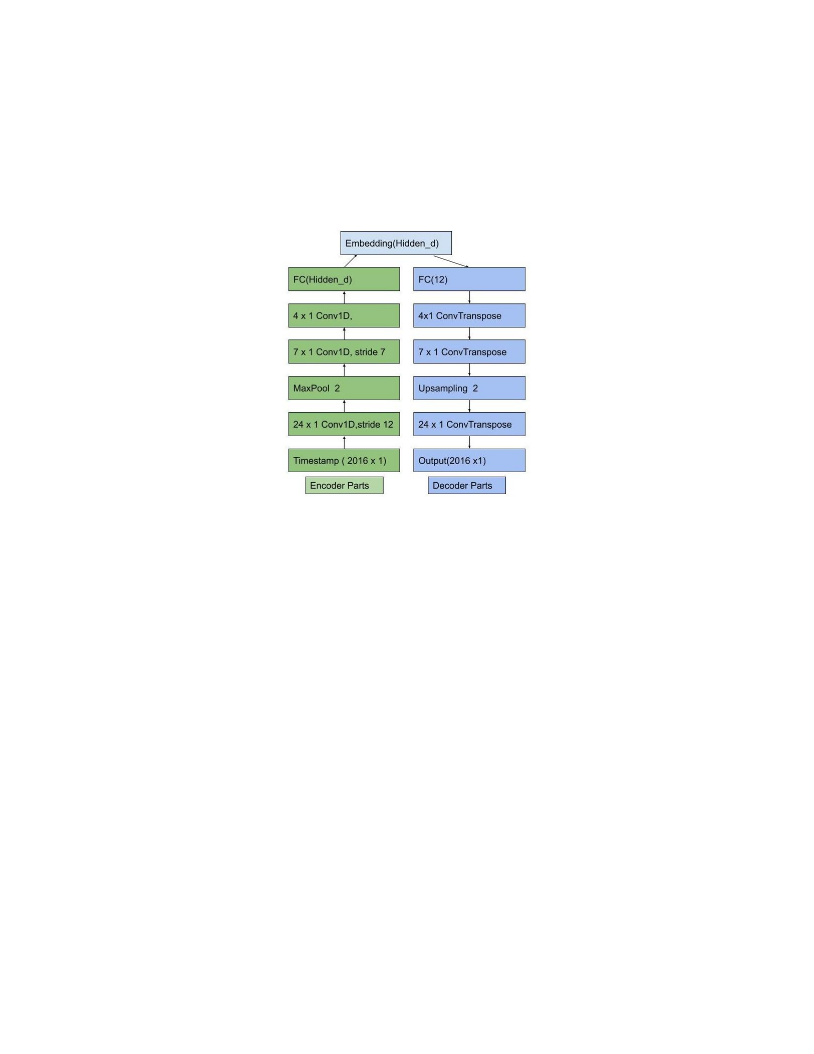
5.3 Proposed Method

An overview of our developed system for accounts clustering in Telegram is shown in

Figure 5.2. In this section, we introduce the detailed methods integrated in the model to

identify accounts belonging to the same user.

Figure (5.3) Auto-encoder Structure

5.3.1 Time Pattern Representation Learning

To construct an attributed network, the first step is to learn the attribution for each node.

For node type ”time pattern”, we need to learn the hidden properties of each timestamp list.

From telegram chat logs, we are able to extract posts of each account as well as

timestamp of each post. Accounts belonging to one user should display similarities in time

pattern for post. The similarity is not just measured by the Euclidean distance of two

timestamp lists. User’s time zone, location, work routine may affect the timestamp list. For

example, some users prefer to post in the morning, some may prefer night and some may

only work on weekdays. There also might exist some relationships between timestamps of

user’s different posts. To gather all of this information into a relational vector whose distance

can represent the similarity level is not an easy task.

In this paper, we propose to build an auto-encoder to learn the hidden properties of

these timestamp lists because we don’t have enough labeled data. Different from other

dimensionality reduction methods, auto-encoder not only reduces dimensionality, but can

also detect repetitive structures[106]. We believe this is a good property for our situation.

Users post the advertisements of their products repeatedly in group chat channels.

In the encoder part, we tried different types of neural networks and experiments in part

4 shows convolutional neural network encoders perform best among all these types of

encoders.

CNNs were well known in the computer vision and machine learning communities[107].

AlexNet shows, for the first time, that the features obtained by learning can transcend

manually-designed features, breaking the previous paradigm in computer vision. [108].Our

CNN encoder shows similar design philosophies with AlexNet.

Figure 5.3 shows the details of each layer in encoder and decoder. First of all, We

preprocess each timestamp list to a vector. Here we only record the timestamp list of each

account from the last 3 month. In total there are 12 weeks which are 2016 hours long. We

use a 2016 × 1 vector to represent the timestamp list, each value in this vector is the number

of posts in that hour. Hour is the smallest time unit we would consider. In our encoder, we

have convolutional layers, max pooling layer and fully connected layer. In the first

convolutional layer, we set the filter’s size as 24 which can convolute timestamps in

consecutive 24 hours. After the max pooling layer, each data is the learned embedding of one

day long. The second convolutional layer’s filter size is 7, which will convolute timestamps in

a week. Followed by the last convolutional layer which will convolute timestamps in 4 weeks.

Decoder’s designs are opposite layers of related encoder layers.

By training the auto-encoder, we get the hidden features we want to measure the

similarity of the timestamp list. The encoder is the model we want to utilize to learn the

representations of timestamp lists. We can get the low dimensional embedding of each

timestamp list by process timestamp list through the learned encoder.

5.3.2 Text Features Extractions

Except for the time pattern, our model leverages the text post by the account as well.

Therefore we also need to learn the representations of post text in group chat channels.

In this paper, we learn the representation of text by a pre-trained language model, BERT.

BERT is designed to pre-train deep bidirectional representations from text by jointly

conditioning on both left and right context in all layers[79]. It’s empirically powerful and

has obtained state-of-art results on several natural language processing tasks. We input one

text to a pre-trained BERT model which converts text to a vector.

5.3.3 AHIN Construction

To describe vendors, time patterns, texts, product-related attributes, and the rich

relationships between them, we propose to use the attributed Attributed Heterogeneous

Information Network (AHIN) for representation.

Attributed Heterogeneous Information Network (AHIN)[109]: Let T = {T1,...,Tm} be a

set of m object types. For each type Ti, let Xi be the set of objects of type Ti and Ai be the set of

attributes defined for objects of type Ti. An object xj of

type Ti is associated with an attribute vector fj = (fj1,fj2,...,fj|Ai|). An AHIN is a graph

G = (V,E,A), where is a set of nodes, E is a set of edge, each represents a binary

relation between two objects in V , and .

To better understand the schema level of the AHIN we built, we provide a meta-level

description.

Network Schema[109,110]: A network schema is the meta template of an AHIN G =

(V,E,A). Let (1) ψ : V → T be an object-type mapping that maps an object in V into its type, and

(2) ψ : E → R be a link-relation mapping that maps a link in E into a relation in a set of relations

R. The network schema of an AHIN G, denoted by TG = (T ,R), shows how objects of different

types are related by the relations in R. TG can be represented by a schematic graph with T and

R being the node set and the edge set, respectively. Specifically, there is an edge (Ti,Tj) in the

schematic graph iff there is a relation in R that relates objects of type Ti to objects of type Tj .

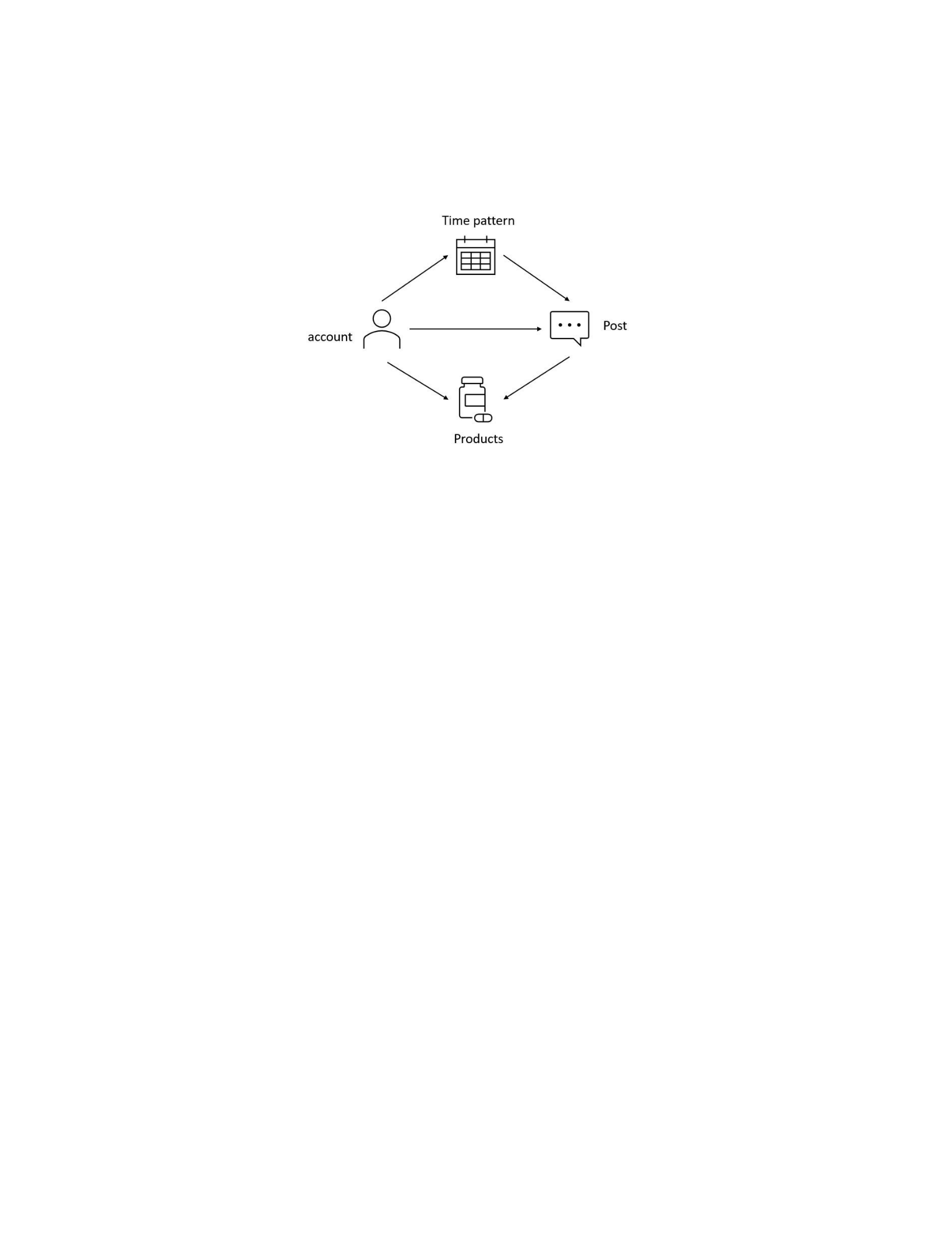
Figure 5.4 shows the network schema of our application. In our network, we have four

node types and five binary relations. Two accounts can be connected via different paths

through our heterogeneous network.

Figure (5.4) Network Schema

Meta path P is a path defined on the graph of network schema TG [111], which include

types, nodes and relations. A meta path is symmetric if the relation defined by it is symmetric.

In our application, we are able to find the same text post by different accounts or same

products by different accounts. Therefore, we can create symmetric meta paths with product

nodes or post nodes as bridges. Figure 5.5 shows the four most meaningful symmetric meta

paths we applied to present relationships between two accounts in Telegram from different

views. MP1 means two accounts are connected by posting the same product in the Telegram

group chat channel. MP2 means two accounts are connected by posting the same text. MP3

denote that two accounts can be linked if they posted the text describing the same product

with similar time pattern. MP4 represents that two accounts can be linked if they post the

same text with similar timestamps.

5.3.4 The User2Vec Model

We present a framework, User2Vec, which is capable of learning account

representations in the attributed heterogeneous network we built. The desirable node

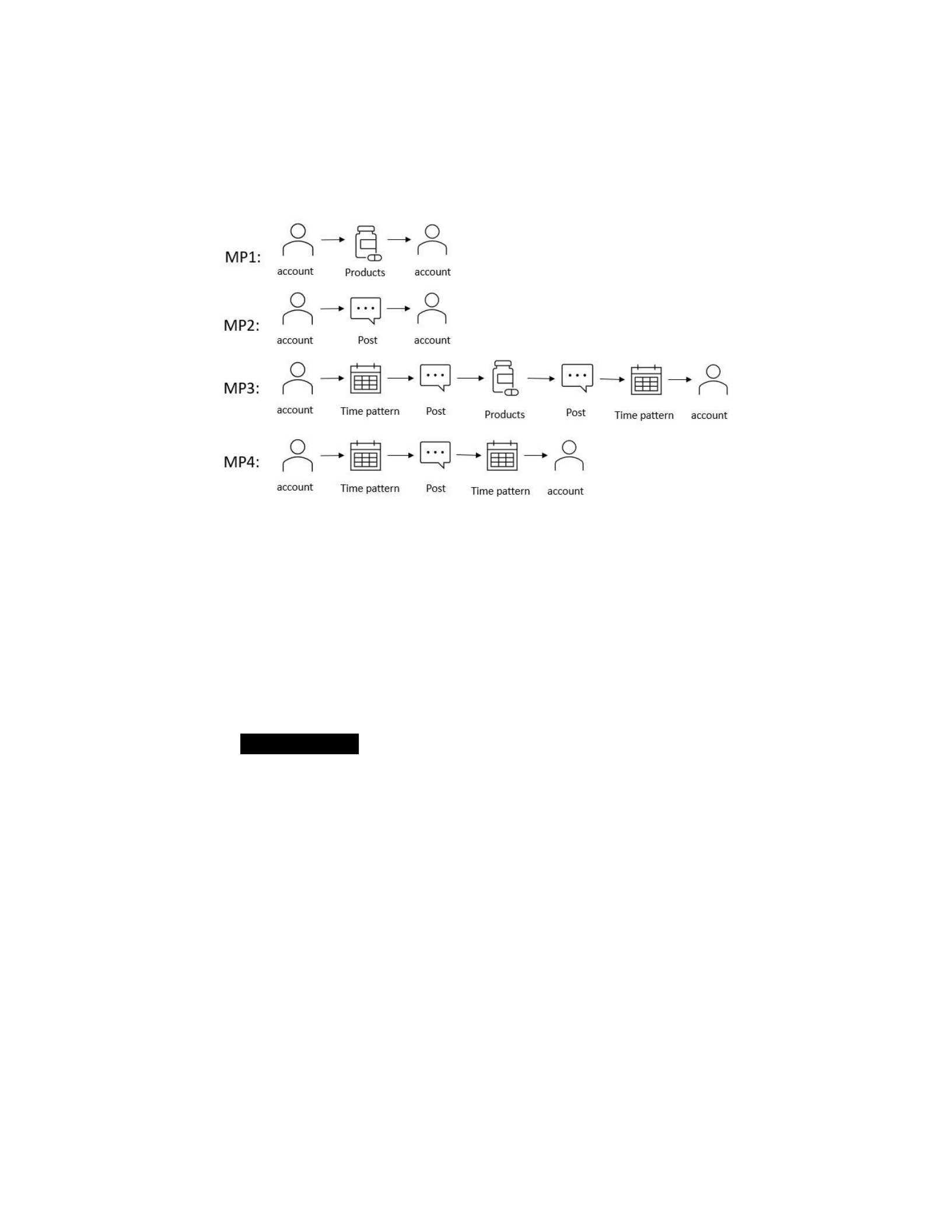
representations should be low dimensional and preserve the context of each node in the

heterogeneous network.

Given a heterogeneous network as input, we formalize the problem of heterogeneous

Figure (5.5) Meta path

network representation learning as follows.

Attributed Heterogeneous Network Representation Learning[112]: Given a

heterogeneous network G = (V,E,A), the task is to learn the d-dimensional latent

representations that are capable of capture the structural and semantic

relations among them.

We first introduce the embedding method for homogeneous networks and

heterogeneous networks. Mikolov et al. proposed Word2Vec which can learn the embedding

of each word from the context in a given text corpus[113]. By applying the same idea,

DeepWalk and Node2vec learn the node embedding from the context of each node in network

[104]. Both methods sample paths from the network through random walks and transfer the

network structure into a skip-gram model and embed the nodes to the low dimensional

vectors. To learning the embedding of heterogeneous network with similar solution,

metapath2Vec extracts the path from meta path of heterogeneous network[112]

In our application, we want to leverage the attribute vector of time pattern and text

nodes. We apply a biased meta path method to guide attributed heterogeneous random

walks. Given a attributed heterogeneous network G = (V,E,A) and a meta-path scheme P : T1

→ T2 → ···Tt → Tt+1 ··· → Tl, the transition probability at step i is defined as:

exists

not exists

0, (vi+1,vti) ∈ E/

where vi represents the the node visited in ith step and ) represents the Tt+1 type

neighbor nodes of vi. In our application, we sample paths from symmetric meta path. If vi in

the first half of meta path, the probability of transition to node in type Tt+1 is inversely

proportional to number of neighbors in type Tt+1. If vi in the second half of meta path, then a

symmetric node of vi+1 exists, which is v0 in our equation. Here we need to calculate the

similarity of vi+1 and v0. sim(fv0,fvi+1 is the similarity calculated by attribute vector of node v0

and node vi+1 A node with higher similarity with v0 will be sampled with higher possibility in

random walk. With this guide, we can generate node sequences which can be the input of

skip-gram model.

5.3.5 Classification Model

In the end of our model, we feed a pair of account vectors to a binary classifier.

We apply a Deep neural network into account embedding, which contains fully

connected layers. The last layer includes two neurons to decide whether the pair of accounts

are from the same user.

5.4 Experiments and Results

In this section, we first compare the performance of representation learning of

autoencoders. Followed by the evaluation of User2Vector in Attributed Heterogeneous

Information Network.

Figure (5.6) Filters Learned by the First Layer of 24-7CNN

Figure (5.7) Filters Learned by the Second Layer of 24-7CNN

5.4.1 Time Pattern Embedding Comparisons

In this set of experiments, we first evaluate the effectiveness of CNN encoder as a

representation learning model.

To fully evaluate the representation learning method, we have downloaded the data from

popular Telegram public channels. We develop a related parser to parse the timestamp list of

each account from Jan-3-2022 to Mar-27-2022. Here we parsed 161797 posts from 7569

accounts. If the timestamp list is too short, we are not able to learn the features of a time

pattern. Therefore, we remove accounts that post less than 10 times.

Due to the anonymity of Telegram, we don’t know which ones are owned by the same

user. After we train the encoders with a parsed timestamp list, we randomly separate the

timestamp list of each account into two sublists equally. By comparing the similarities

between those sublists, we are able to evaluate the effectiveness of the learned encoder.

Here we compare four types of encoder and manually-designed features.

Models Here we compare four types of encoder and manually-designed features

• CNN auto-encoder Details of encoder and decoder design are displayed in Figure 5.3.

In our encoder, we have convolutional layers, max pooling layer and fully connected

layer. Decoder’s designs are opposite layers of related encoder layers.

• RNN auto-encoder RNN auto-encoder’s design is similar to the CNN auto-encoder,

where we replace convolutional layers with simple RNN layers.

• LSTM auto-encoder LSTM auto-encoder’s design is similar to the RNN autoencoder,

where we replace simple RNN layers with LSTM layers.

• FC auto-encoder FC represents a fully connected layer. In FC encoder, we have three

layers of fully connected neural networks.

• Manually-designed Features We also test the manually selected features. In our

design, each timestamp list is converted to a 24+7 = 31 dimensional vector. It includes

the number of posts in 24 separate hours and number of posts from Monday to Sunday.

DataSets Here we use 2 types of data

• Telegram Data We parse the timestamp list of each account from Jan-3-2022 to Mar-

27-2022 and randomly separate the timestamp list into two sublists.

• Synthetic For each timestamp list we parse from Telegram, we create a synthetic

timestamp list. We manually replace each timestamp with a random hour in the same

day or same hour on a random day of this week.

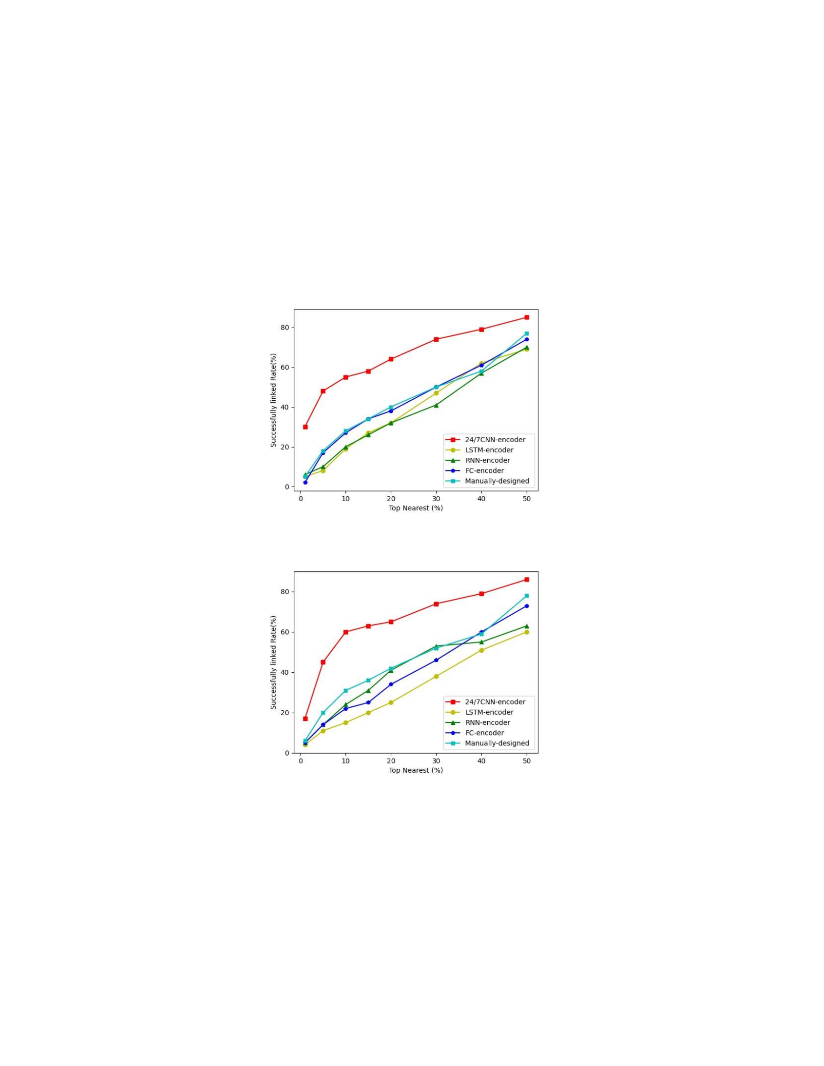
Evaluation Metric The aim of our experiments are trying to see whether the learned

embedding can be used to measure the similarities of timestamp lists. Consider the learned

embedding of these models in different scales. Here we use the percentage value as an

evaluation metric instead of Euclidean distance of vectors. We first set a threshold λ%. Here

we calculate the Euclidean distance between learned vectors and link each account with the

top nearest λ% accounts. We use the percentage of successful linkage as Evaluation Metric.

(a) on real data

(b) on synthetic data

Figure (5.8) Comparisons of Embedding

Figure 5.3 shows the experiment’s result. We start from λ%, which means we link each

account with λ% nearest 1% accounts. We can see embedding learned by CNN encoder can

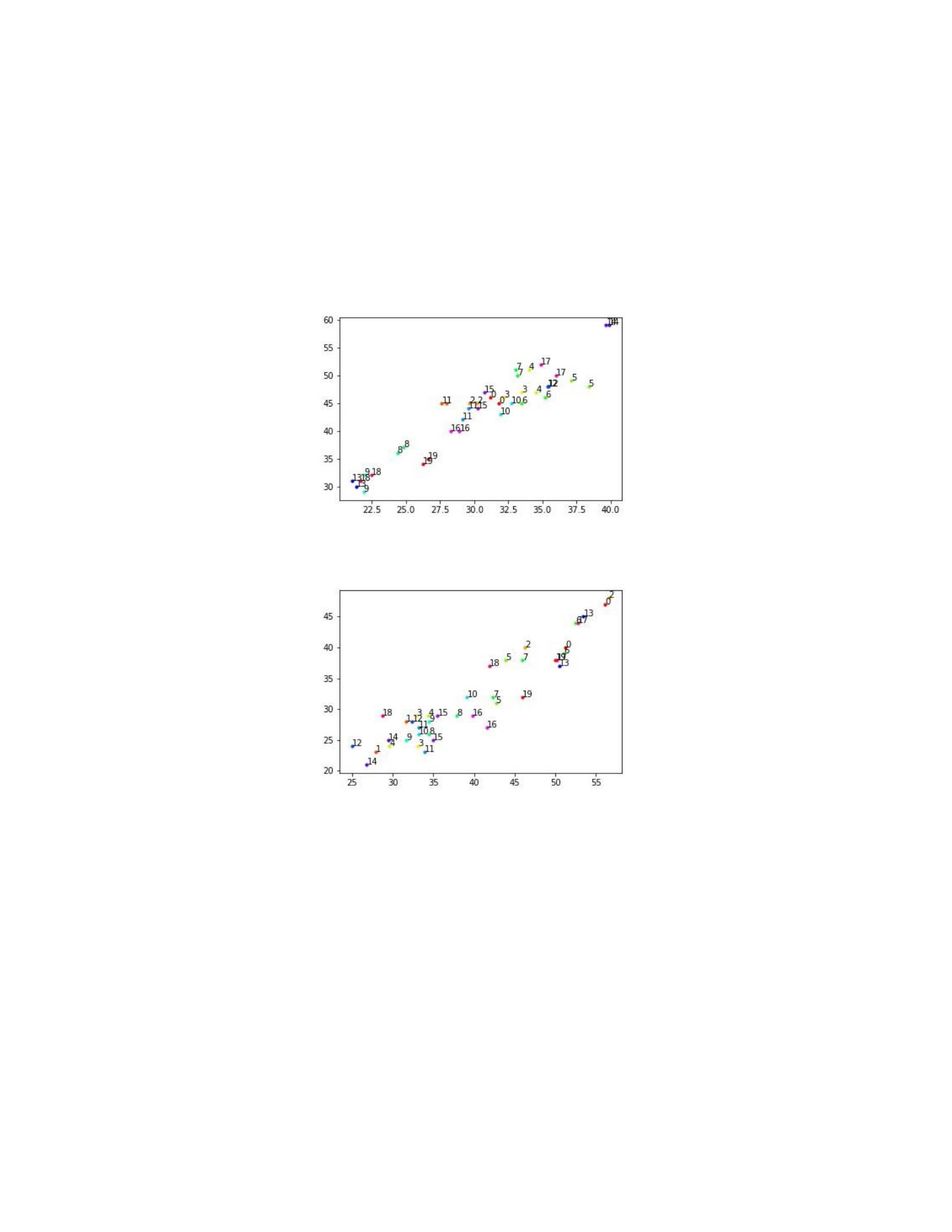
successfully link 28% of all account pairs, which is much higher than the result from RNN

encoder, LSTM encoder, Fully-Connected encoder and manually designed features.

To get the intuitive sense of embedding of CNN encoder. We convert a vector of 20 pairs

accounts into a 2 dimensional vector. Figure 5.9 shows the result and we can see accounts

from the same user are close to each other.

(a) on real data

(b) on synthetic data

Figure (5.9) Learned Representation of 24/7 CNN Encoder

5.4.2 User2Vec Performance

To evaluate the performance of our System, we compare three different networks. Not

only the attributed heterogeneous network, we also build heterogeneous network and

homogeneous network with the same data.

For the heterogeneous network, we didn’t attach attributes for timestamp nodes or post

type nodes. We use metapath2Vec to sample the path from the network, which will sample

meta paths we extracted from the network schema, however, the possibility of the next node

will not be affected by the attributed vector [112].

For the homogeneous network, we treat all the nodes as the same type and we sample

the paths with DeepWalk which utilizes random walkers without following any meta

paths[104].

We compare the performance of these three models with two community data from

telegram. One is scam related channels and another one is drug related channels.

Table (5.1) Comparisons of Different Models

Channels

AHIN+ User2Vec

HIN+ metepath2Vec

Homo network+ DeepWalk

Scam

0.785

0.696

0.6875

Drug

0.8025

0.713

0.694

Table 5.1 shows the accuracy of trained classifiers of three different models. We can see

that our model which leverages most information from the network can achieve the best

accuracy.

5.4.3 Case Study

Table (5.2) Post Frequency of Account1 and Account2

Account1

Account2

date and time

Frequency

date and time

Frequency

04/16, 9pm

04/14, 8pm

04/16, 10pm

04/14, 9pm

04/16, 11pm

04/14, 10pm

04/17, 12am

04/14, 11pm

04/17, 1am

04/15, 12am

04/17, 2am

04/15, 1am

04/15, 2am

04/15, 10pm

04/15, 11pm

04/16, 12am

04/16, 1am

04/16, 9pm

04/16, 10pm

04/17, 12am

We also tried unlabeled data from telegram to gain deeper insights of our proposed

model. For the pairs of accounts that are defined as one user, we are with high confidence

(a) Post of Account1 (b) Post of Account2

Figure (5.10) Post Text of Detected Account Pair Account1 and Account2

that they are the same individual by manually checking. For example, Figure 5.10 shows the

post by these two accounts, we can see the text is extremely similar. Both accounts post a lot

of times. To better show the timestamp list, we count the frequency of posts in each hour and

display the result in Table 5.2. We can tell these two accounts are very active from 10pm to

3am.

5.5 Conclusion

In this paper, we study the problem of how to identify the accounts from the same user

in Messaging Software. After we parse the chat logs from public channels, we first extract the

features of the timestamp list and text post of each account. We learn the embedding of

timestamp list through a novel 24/7 CNN encoder and the embedding of post through pre-

trained self attention transformer Bert. We further proposed the User2Vec model, where we

sample the meta path from AHIN we build and feed the paths that capture the structure and

semantic relations to the skip-gram model. In the end, we train a binary classifier to classify

each pair of accounts to decide whether they are the same user or not. Comprehensive

experimental results have demonstrated the effectiveness and efficiency of the proposed

model.

PART 6

CONCLUSION

In this dissertation, we present our research on how to combat cyber crime by attacking

privacy provided by darknet and IM softwares.

For darknet, we firstly analyze Bitcoin transaction patterns behind cryptomarkets and

discover interesting transaction patterns and management mechanisms from different

cryptomarkets. The results demonstrate that the privacy protection mechanism in Bitcoin is

still vulnerable in terms of simple analysis. For markets like the Wall Street market, feedback

reviews released on web pages are highly related with public Bitcoin transactions in terms

of timestamp and money value. An adversary can extract valuable information for analyzing

the activities. Based on the transactions pattern we discovered from darknet markets, we

further proposed a method to uncover the Bitcoin addresses of a vendor in darknet by

matching their feedback reviews with public bitcoin transactions. We first proposed the

metric which is maximum coverage of reviews by a Bitcoin address. A Bitcoin address’s

transaction history can match maximum reviews owned by the vendor with the highest

possibility. In our model, we construct a K-D tree to efficiently match Bitcoin transactions to

feedback reviews based on timestamp and money value. The problem is proved to be NP

hard. By utilizing the sub modular property of our objective function, we get the address set

with a greedy algorithm that can achieve near-optimal with theoretical guarantee. We further

develop a Cost-Effective Address Searching(CEAS) algorithm that can speed up the process

by pruning the search space effectively. Comprehensive experiments on both real and

synthetic datasets demonstrate the effectiveness and efficiency of our methods.

For IM software like telegram, vendors broadcast their products through related group

chat. A group in such IM softares normally contains thousands of members including both

vendors and customers. Learning infectivity graphs from these group chats can help us

analyze organizations and supply chains behind these illegal products. We propose an

effective model to discover hidden networks of influence between members in a group chat.

We model message sequences to a multi-dimensional Hawkes process by treating the whole

chat history as sequential events. The triggering pattern between members inside a group

can help us extract influence between different individuals. In our model, we apply NLP

techniques to embed the text information of messages to get a more precise relationship

between members in group chat. We learn the influence graph by applying an expectation–

maximization(EM) algorithm on our text biased multi-dimensional Hawkes Process. And we

conduct experiments with designed metrics on synthetic data and real data with different

models.

We further study the problem of how to cluster the accounts from the same user in

Messaging Software. We learn the embedding of timestamp list through a novel 24/7 CNN

encoder and the embedding of post through pre-trained self attention transformer Bert. We

further proposed the User2Vec model, where we sample the meta path from AHIN we build

and feed the paths that capture the structure and semantic relations to the skip-gram model.

In the end, we train a binary classifier to classify each pair of accounts to decide whether they

are the same user or not.

Students also viewed