Introduction Summaries Foundation Section One Eliminating Extreme Poverty Has Been A World Priority

Introduction Summaries Foundation Section One Eliminating Extreme Poverty Has Been

A World Priority

Foundation section one eiminating extreme poverty has been a world priority for some

time, highlighted by its prominence in the Millennium Development Goals. Significant

progress has been made on this front, but we still have a long way to go. Combating

poverty efficiently requires an understanding of the root causes of poverty in the socio-

economic context it occurs in order to tailor poverty alleviation programs to the needs of

poor. In this dissertation, we (referring to myself and the significant and essential

collaboration with my committee) contribute to this substantial task by analyzing

poverty reduction programs in empirical and theoretic contexts.

Poverty reduction programs come in many forms, which can and should be

tailored to address the context where poverty is being combatted. There is no overarching

solution, as the context of the socio-economic system directly impact how effective

various strategies will be. While there are far too many potential aid strategies to detail

here, we provide a brief overview of some of the methods available in order to discuss

their applicability to combat poverty for the case studies in Tanzania and Ethiopia, which

we look at in this dissertation.

Microfinance, providing small-scale financial services to low-inomce populations,

has been a popular method of reducing poverty since the 1970s (Marr, 2012). While

originally used to provide mostly small scale loans in an attempt to provide the capital

needed as well as a means of protecting against negative shocks, more recently these

institutions have been moving towards offering micro-savings programs as well (Rooyen,

2012). These programs have been popular as they provide access to capital with which to

start up small businesses or invest in productive capital such as fertilizer and farming

equipment. This is especially relevant to the poverty trap discussion, which we go into in

sections 3 and 4 as one theoretic cause of persistent poverty is the inability to afford

productive assets, which would enhance long term outcomes. In fact, much of the

theoretic poverty trap literature requires assuming no access to credit markets for this

reason. In a review of microfinance in sub-Saharan Africa, Rooyen (2012) finds overall

positive results, but also there are cases where it provides significant harm to those

receiving micro-loans. Rooyen finds micro-saving to have a more consistent benefit to

recipients than the micro-loans, which is a trend that microfinance institutions have been

moving towards recently. In addition to income impacts, there also appears to be

significant benefits to other areas such as child education and empowerment of women,

the latter largely attributed to many microfinance institutions primarily providing services

to women in the household (Marr, 2012).

Another popular form of aid has been direct payments to households so long as

the households follow some requirements, known as Conditional Cash Transfers (CCT).

These programs provide aid while incentivizing behaviors which can lead to a reduction

in long-term poverty such as increased education and better health practices. These

programs have been especially prevalent in Latin America and, more recently, have been

used in Asia and Africa (Evans et al., 2016). In a review of 13 CCTs in Latin America,

Ranganathan and Mylene (2102) show overall these programs have been effective at

increasing health behaviors as well as providing short-term aid in the form of payments.

By requiring healthy behavior, these programs enhance the productivity of the recipients,

which provides a long-term benefit. This is especially true when trying to combat

intergenerational poverty. By incentivizing households to send children to school and

attend health facilities at young ages, such as in the CCT we look at in chapter 2, it is

hoped that the children of aid recipients will be better able to provide for themselves in

the future, thus reducing the need for poverty reduction programs in the future. While

CCTs appear effective at reducing poverty and enhancing health and education outcomes,

there is some concern of unintended spillovers in terms of how individuals interact with

the local environment.

In section 2, we analyze the unintended spillovers of poverty reduction program

on local fisheries in rural Tanzania. If unaccounted for, spillovers may have adverse

effects on the long term well being of population reducing the effectiveness of aid. This is

especially true in rural settings where impoverished populations live on fragile land and

have livelihoods that depend heavily on local environment (Barrett et al., 2011; Barbier,

2010). Poverty alleviation should take into account the complex feedbacks between the

environment and socio-economic system to avoid negative unintended consequences. In

extreme cases, poverty reduction policies with severe negative impacts on local

environmental amenities may result in short lived gains to wellbeing if they result in the

exasperation or the beginning of a ‘poverty-environment trap’, where poverty and

environmental degradation become self-reinforcing (Barbier (2010).

There is mixed evidence for whether poverty reduction leads to negative impacts

on local environmental amenities (e.g. Foster and Rosenzweig, 2003; Zwane, 2007; Alix-

Garcia et al., 2011; Hannah and Olivia, 2015) depending on the context being studied and

the environmental amenity being studied. While there have been large strides in

understanding how poverty reduction policies spillover into some resources, most notably

forests and timber products (Koop and Tole, 1999; Martinez et al., 2002; Culas, 2007;

Zhou, et al. 2011), little has focused on how poverty reduction programs impact

dependence on local fisheries. We fill this gap in the literature by looking at a CCT

program in Tanzania and analyze the impact of program participation on demand for

marine and freshwater seafood as well as household income from fishing. Our data come

from a World Bank pilot study which implemented a conditional cash transfer (CCT) to

households in eighty villages within three districts from 2009-2012 (Evans et al., 2014).

In line with much of the world’s fisheries, Tanzania’s fisheries are experiencing

increased pressure and are at risk of overexploitation both inland (Ogutu-Ohwayo, 1990)

and in coastal regions (Berachi, 2003; Silva, 2006). Especially in the coastal regions,

fisheries management programs have been utilized to try to enhance the sustainability of

local fisheries through a combination of marine protected areas in conjunction with ways

of promoting alternative livelihoods to reduce pressure on the fisheries (Berachi, 2003).

Since there is currently activity to push households away from fishing in many areas, it

may be counter productive if poverty reduction strategies have spillovers which increase

demand for seafood and/or increase the number of households who earn income from

fishing.

The CCT targeted poor and vulnerable households and was designed to provide

aid to these vulnerable populations as well as promote health and education in three rural

districts of Tanzania: Bagamoyo (~70 km from Dar es Salaam), Chamwino (~50 km from

Dodoma), and Kibaha (~35 km from Dar es Salaam). The populations of these districts

depend largely on farming, both subsistence and cash crops, with over 32% of

households reporting sale of crops as their primary source of income (Evans et al., 2014).

Only a small percentage of households report fishing income as either their primary or

secondary source of income for this sample, so we are not looking at fishing villages in

this study, but rather farming communities which may have access to fishing to

supplement income. Rural poverty in Tanzania is a long-standing problem with an

estimated 39% of its rural population being poor as of 2000, compared to 24% of its

urban citizens (Ellis, 2003). Thus, many of the poverty reduction programs in Tanzania

have a focus on the rural areas.

The CCT program we look at in chapter 2 targeted the poorest individuals within

the communities to be eligible for program participation based on income/expenditure

surveys and a final selection process conducted by community leaders. Of the sample,

over 90% of households had unimproved floors and under 40% had access to piped water

or had an improved roof (Evans et al., 2014). The program required young children (0-5)

to visit health care facilities 6 times a year and elderly to visit at least once a year while

children between the ages of 7-15 had to maintain an 80% school attendance to be

eligible for payments. The main livelihood for those in the study was farming with 90%

of adults performing some agriculture (Evans et al., 2014). The authors report most crops

were grown for food, a large portion of households (42%) report the main source of

income was from selling food or cash crops. As the study targeted the most vulnerable in

the villages, few households own livestock other than chickens or other durable assets

and less than 2% reported savings of any kind.

The study conducted a randomized control trial designed to analyze the

effectiveness of implementing CCTs in Africa, while much of the previous usage of

CCTs had been conducted in Latin America and Asia. We exploit the randomized control

trial that was implemented for the first stage of the CCT to assess the impact of the CCT

on pressures of local fisheries. We look both at whether increased incomes lead to a

higher demand for seafood products as well as if additional income causes a shift away

from farming towards fishing. Typically demand for seafood products tend to rise with

wealth, which could increase pressures on local fisheries. We find a positive treatment

effect on both demand for seafood products and number of households earning income

from fishing activities. Additionally, we find heterogeneous wealth effects as poverty

reduction policies likely have a systematically different impact on households, which is

correlated with household wealth. Lastly, we find a significant lag between program

participation and observable spillovers suggesting the need for assessment over longer

time frames to ensure spillovers are identified when they exist.

The next two sections look at poverty traps, in essence how households appear

stuck in poverty over time. We use data from the Borana Plateau of southern Ethipoia to

study this phenomenon. In section 3 we present a general poverty trap model loosely

based on this system and section 4 atempts to empirically identify poverty traps using

data of herd sizes from Boran pastoralists. We have 17 years of data across four villages

in the Borana Plateau of southern Ethiopia, an important rangeland for Ethiopia with

livestock from this region supplying various domestic and export markets (Coppock et

al., 2014). The arid climate of the region makes crop production relatively unproductive,

which is why the dominant livelihood has been pastoralism, especially cattle, which has

been prominent in the region for many generations. However, increased pressures due to

rising populations in the region and a drier climate have led to increased degradation of

rangelands and decreased livestock productivity (Lybbert et al., 2004; Soloman, 2006;

Coppock et al., 2014). More recently, there has been growing adoption of non-pastoral

livelihoods increasing the diversification of income streams, especially amongst younger

households (Berhanu et al., 2007). As the lands are becoming less productive, it is also

having to support larger populations, which increases the pressure on the fragile

rangelands (Coppock, 2016). The rangeland has been typically unmanaged and has

recently experienced bush encroachment and gullying due to the additional pressures and

changing environmental conditions, which has led some to propose a more active

management of these rangelands to promote sustainable pastoralism (Coppock, 2016).

Along with the changes associated with decreased rainfall and reduced herd sizes

amongst pastoralists that has been observed over time for this region, between 1983-85

there was a severe famine largely brought about by civil turmoil in Ethiopia combined

with severe drought resulting in substantial livestock loss (Desta and Coppock, 2004).

This famine had widespread effects across the country, but the Boran pastoralists were hit

particularly hard with nearly 10% of the population moving to relief shelters during this

period (Lindtjørn, 1990). This period certainly represents a major shock to the productive

capacity of the Boran pastoralists, which we can clearly see in terms of a reduction in

household herd sizes after this period. This process of shocks and rebuilding is not

uncommon for pastoralists, there is a tendency for drought and other die offs to reduce

herd sizes followed by a rebuilding of herds during good years (Lybbert, 2004).

The pastoralism of the Borana Plateau has been a focal point of the poverty trap

literature (e.g. McPeak and Barrett, 2001; Lybbert et al., 2004; Barrett 2006; Toth, 2014),

along with similar setting in other arid and semi-arid dry lands of east and southern

Africa where semi-mobile pastoralism is the primary livelihood. This system is an ideal

study location due to its reliance on one productive asset (the herd) and lack of access to

alternative livlihoods, which we disucss in more detail in section 3. Most importantly

there is a more productive livelihood (mobile pastoralism), which is only accessable with

a large enough herd size. Thus, there is a clear and visable mechanism, which could

explain a poverty trap in this system.

Semi-mobile or transhumant pastoralism occurs when households’ move herds

between pastures, especially during the dry seasons, while maintaining a permanent

home. Typically the herd is broken down into two sub-herds: the warra herd consisting

of milk cows and calves under two years old, which remains near the home, and fora

herd, which migrates between pastures and water sources consisting of older immature

cattle, dry cows and bulls (Lybbert et al., 2004; Soloman, 2006). Accessing pastures

away from the immediate village requires a large enough fora herd to support the herders

who rely heavily on meat and blood from their animals during the long migrations

(Lybbert et al., 2004). Thus, mobile pastoralism requires a minimum herd size. When

herds drop below this level, the household must resort to sedentary pastoralism, which is

far less productive and associated with significantly higher rates of poverty (Little et al.,

2008; Toth 2014).

This represents multiple production technologies (mobile and sedentary

pastoralism), where the more productive technology requires a minimum wealth level to

access. This is one of the theoretic mechanisms that can cause a multiple equilibrium

poverty trap, which we discuss in section 3. Another desirable feature of this system, in

the context of identifying poverty traps, is wealth is almost exclusively maintained in the

form of the herd with little to no access to financial markets.

In chapter 3, we expand upon our theoretic understanding of how to provide

optimal aid to populations experiencing a poverty trap. A poverty trap is characterized by

self-reinforcing mechanisms causing poverty to persist (Azariadis and Stachurski, 2005).

In this chapter we focus on a specific case of poverty trap where wealth dynamics result

in multiple dynamic equilibria each with its own basin of attraction (in essence pulling

wealth towards it over time) separated by a critical wealth threshold known as the

Micawber Threshold. In this context, once people fall into poverty they are highly likely

to remain impoverished in the future due to a lack of productive assets and means to

accumulate them. In such cases, individuals are very unlikely to surmount the Micawber

Threshold on their own and require external aid in order to escape poverty.

We expand upon this literature by analyzing how the level of aid affects the cost

and effectiveness of poverty reduction. Specifically we seek to answer the question of

whether aid should target the Micawber Threshold. Barrett (2005) suggests for aid to be

effective it must ensure wealth surmounts the Micawber Threshold, however, Barrett

only shows this for the deterministic case. On the other side, Plucinski, Ngaonghala, and

Bonds (2011) have shown aid set below critical thresholds can lead to escaping poverty

trap, but do not attempt to determine if this is optimal.

We present a poverty trap model and use numeric simulation to show optimal aid

typically must be set above the Micawber Threshold when combating the multiple

equilibrium poverty trap. When aid is set below the Micawber Threshold, typically

results in a higher cost of poverty reduction coupled with higher rates of poverty, clearly

an undesirable outcome. This arises due to an aid trap forming when aid is set at a level,

which households can not maintain over time, as they are still in the basin of attraction of

a low wealth equilibria, while not being set high enough to significantly escape poverty

in the future. Additionally we show the optimal aid level is largely determined by the cost

of providing aid and the level of poverty as well as the weight a society places on

poverty, which together can be thought of as the social cost of poverty, plays only a

secondary role. This arises due to the coupled relationship between cost and level of

poverty, which arises due to the aid trap. This chapter highlights the importance of

understanding the dynamic process leading to chronic poverty based on numeric

simulation and provides a theoretic starting point with which to make policy decisions

when a multiple equilibrium poverty trap exists.

However, the identification of multiple equilibrium poverty traps has numerous

challenges (Barrett and Carter, 2013; Nashold, 2013), which limits the applicability of the

theoretic results. Identifying the root cause of poverty is a necessary step to provide

optimal policy. In section 4, we introduce two novel tests to surmount some of the issues

associated with empirically identifying multiple equilibrium poverty traps by testing for

implications of poverty traps rather than directly identifying the poverty trap itself. The

first issues we circumvent are a lack of observations around the Micawber Threshold,

which is a necessary feature of the multiple equilibrium poverty trap as it is an unstable

dynamic equilibria with stable equilibria on either side pulling wealth away from the

Micawber Threshold over time. The second issue is many empirical test for multiple

equilibrium poverty traps do not allow for heterogeneity amongst a population and

assume a single underlying asset dynamic (Jalan and Ravallion, 2004; Nashold, 2013),

which is unrealistic as individual ability (Ikegami et al., 2016).

We first test for mean reversion at the individual level using a variance ratio test,

which has been widely used in the finance literature to test whether financial assets

follow a random walk (e.g. Lo and MacKinlay, 1988). By testing at the individual level

opposed to the aggregate level, we can allow for heterogeinity across individuals.

Additionally we perform a mixture model designed to pick up clustering of data

consistent with a multiple equilibrium poverty trap. However, this test does require

assuming equilibria are homogeneous across the population. The clustering of data is a

necessary feature of equilibria at the aggregate and village levels. The downside to our

tests, is we cannot distinguish between whether a multiple equilibrium poverty trap exists

or an alternative hypothesis of club convergence where both mean reversion and the

equilibria are caused by each individual having access to one of the equilibria. Thus our

test is designed as a falsification test to determine when a poverty trap cannot be present.

When we apply our empirical tests to our data on the Boran pastoralists, we find

no evidence of a poverty trap. This contradicts previous findings of Lybbert et al., (2004).

In their paper, the authors use a direct test designed to fit a curve to the data to locate the

Micawber Threshold and non-convex1 wealth dynamics associate with a multiple

equilibrium poverty trap. We find this results is spurious likely caused by overfitting due

to some clustering in the data around the Micawber Threshold they identify. Their

analysis does not take into account the likelihood of data being present. If a Micawber

Threshold exists, there should be few observations nearby that level of wealth, which

they fail to account for. This chapter highlights the importance of multiple and rigorous

tests in order to identify the underlying poverty dynamics of a socioeconomic system, as

applying poverty alleviation strategies assuming a poverty trap exists when it does not

may lead to inefficient policy decisions.

The remainder of this dissertation is organized as follows. Chapter two evaluates

the spillovers of a cash transfer program on the dependence of local fisheries. Chapter

three introduces a poverty trap model and shows a “guaranteed wealth” aid policy should

be set at the Micawber Threshold. Chapter four and five expand on this model by

breaking down the cost of providing a guaranteed wealth at the Micawber Threshold into

the cost of providing a “cargo net” and the cost of providing a “safety net” and introduce

a method for estimating these costs with chapter four focusing on cargo nets and chapter

five focused on the safety net. Chapter six concludes this dissertation.

1. Impact of Poverty Reduction Programs on Dependence of Local Fisheries

1.1 Introduction

The relationship between poverty and environmental quality has been a long-standing

question. Especially in rural settings, impoverished populations tend to live on fragile

land and have livelihoods that depend heavily on local environment (Barrett et al., 2011;

Barbier, 2010). There is a complex relationship between the environment and the

livelihoods of the people living in these areas. A central question at this environment-

poverty nexus is whether poverty reduction programs impact environmental quality in the

surrounding area. It is unclear whether reducing poverty will put additional strain on local

environmental amenities due to increased demand for resource intense products or

potentially lead to households investing in environmental quality and reducing

environmental damages (Alix-Garcia et al., 2011). The current literature is ambiguous

about whether poverty reduction programs have spillovers into the realm of

environmental quality as well as the direction of the impact if one exists (e.g. Hannah and

Olivia, 2015; Zwane, 2007; Foster and Rosenzweig, 2003).

Understanding how poverty reduction programs impact local environmental

quality can have major implications especially when livelihoods depend on the local

environment. Reductions in poverty from these programs may be short lived if they

degrade the ecosystems which the impoverished populations depend upon and may result

in the exasperation or the beginning of an ‘poverty-environment trap’ as described by

Barbier (2010), where poverty and environmental degradation become self-reinforcing.

The environmental and economic conditions are likely to greatly impact how poverty

reduction programs may impact local ecosystems. The livelihoods of the impoverished

population and how they change in response to poverty reduction programs will greatly

influence whether poverty reduction leads to environmental degradation or improvement.

The livelihoods of the target population will also impact which environmental amenities

are likely to be affected.

While there have been large strides in understanding the relationship of how

poverty reduction policies spillover into some resources, most notably forests and timber

products, little has focused on how poverty reduction programs impact dependence on

local fisheries. We fill this gap in the literature by looking at a Conditional Cash Transfer

(CCT) program in Tanzania and analyze the impact of program participation on demand

for seafood2 and earning income from fishing. We exploit a randomized control trial that

was implemented for the first stage of the CCT and find a positive treatment effect on

both demand for seafood products and number of households earning income from

fishing activities. Additionally, we highlight the importance of looking at heterogeneous

wealth effects as poverty reduction policies likely have a systematically different impact

on households depending on their wealth. Lastly, we find a significant lag between

program participation and observable spillovers indicating the importance of longer

period data sets to be sure any effects are picked up on.

1.2 Background

Understanding the complex relationship between income and environmental degradation

has been a long-standing question with important implications for both poverty reduction

and environmental management. The topic largely began with Grossman and Kruger’s

2 The definition of seafood we use includes all marine and freshwater species.

(1991) adaptation of Kuznets (1955) theory, now known as the Environmental Kuznets

Curve (EKC), which predicts an inverted u-shaped relationship between wealth and

environmental quality, implying as a poor country gains wealth it will degrade its local

resources in the process of development up to a point where it is wealthy enough to

afford to invest in environmental quality.

There is mixed evidence of the existence of the EKC and depends largely on the

type of pollution being considered. Grossman and Krueger (1995) use data from a panel

of many cities in different countries and find evidence in favor of the EKC for air

pollution and river water quality. Local air pollution has been one of the more widely

studied indicators used to identify the EKC with a large body of supporting evidence (e.g.

Seldon and Song, 1992; Cole et al., 1997), however, pollutants with a longer term or

dispersed damages appear to monotonically increase with per capita income (Arrow et

al., 1995; Cole et al., 1997). There has even been some contention over previous findings;

Stern (2004) suggest much of the evidence in favor of the EKC hypothesis may have

issues with serial dependence in time series data and/or omitted variable bias and find,

once these are correctly accounted for, most pollutants and waste flows are increasing

with per capita income. Deforestation is another localized environmental quality indicator

with mixed evidence in favor of the EKC hypothesis (e.g. Koop and Tole, 1999; Martinez

et al., 2002; Culas, 2007; Zhou, et al. 2011).

While highly debated, both in theory and with contradicting empirical evidence

(e.g. Stern, 2004; Li et al.; 2007; Choumert et al., 2013), this idea is still prominent in the

poverty-environmental quality discussion where there is a concern that increasing wealth

amongst poor populations will lead to increased pressure on local natural resources. Thus,

there may be unintended negative consequences to providing aid to impoverished

populations, which are largely not considered when governments are implementing

poverty-reduction policies (Alix-Garcia et al., 2013). Understanding the complex

relationship between poverty and natural resource usage may shed light on whether

reducing poverty will necessarily reduce environmental quality or if win-win solutions

exist in terms of poverty reduction and environmental quality.

A large portion of this literature has focused on deforestation and forest

degradation as it is an issue in much of the developing world and, especially in the case

of deforestation, highly visible issue. There is mixed evidence concerning the actual

effect of poverty reduction on deforestation rates, which may be largely due to differing

socio-environmental conditions of the study area. Foster and Rosenzweig (2003) find no

evidence increasing income leads to afforestation in open economies where there is a

weak link between demand for forest products and forest cover, but in a closed economy,

they find a positive relationship between income and forest cover. In contrast, Zwane

(2007) find evidence of a positive, but decreasing, relationship between income and

deforestation rates in Peru, consistent with the EKC. Similarly, Alix-Garcia et al. (2013)

find poverty reduction has negative spillover effects in terms of increasing deforestation

in Mexico. Poor households tend to switch to more land-intensive farming activities in

response to the increased income.

The economic and environmental contexts are important to consider as they

pertain to potential livelihoods. Zwane (2007) and Alix-Garcia et al (2013) focus on

deforestation driven largely by households clearing land for agriculture in Peru and

Mexico respectively. This is a prominent concern in places where populations live near

established forests, which are suitable for farming or pasture lands with access to markets

to sell farm products. In other contexts, the demand for forest products come in the form

of extractive behaviors such as fuel wood harvesting, which has been a principle concern

in places such as India (e.g. Foster and Rosenzweig, 2003), China (e.g. Demurger and

Fournier, 2011) and Africa (e.g. Adeoti et al., 2001).

The choice of fuel has numerous health and environmental consequences. Low

quality cooking fuels such as dung, wood, and charcoal can have serious negative health

effects resulting in lower productivity workers, especially when burned indoors as is

typical in many developing countries (Bruce et al., 2000). In addition to health effects,

fuel choice impacts demand for local ecosystem services in the form of harvesting wood

and charcoal from local forests (Demurger and Fournier, 2011). Thus there may be both

an environmental and health benefit associated with households switching away from

these fuel sources. The “Energy-Ladder” hypothesis is as a household’s wealth increases

it shifts towards consuming higher quality fuels (Hanna and Olivia, 2015; Demurger and

Fournier, 2011). If fuel wood is an inferior good, that is to say the use decreases as

income rises, as the Energy-Hypothesis states, we would expect to see poverty reduction

programs result in a lower usage of fuel wood as other, more desirable, fuels become

affordable.

There is mixed empirical evidence about how poverty reduction affects demand

for fuel wood. Hanna and Olivia (2015) show a wealth effect increases aggregate fuel

usage with little substitution towards cleaner fuels in India suggesting an increase in

income will likely put increased pressure on local forests. The authors found a relative

increase in the use of dirty-burning cow dung, which was likely due to the income

increase for households (as part of an aid program) was in the form of cattle. In contrast,

Demurger and Fournier (2011) show firewood is an inferior good in rural China. As

wealth increases, they find significant switching behavior towards cleaner fuels

indicating a reduction in poverty would result in lower harvesting pressure on local

forests. The discrepancy may depend on other factors such as relative price and

availability of substitutes, which is highly influenced by access to markets.

These studies highlight the importance of understanding the economic and

environmental conditions when trying to determine how poverty reduction policies will

impact environmental quality. The linkages between poverty and demand for local

ecosystem services can come from both livelihoods (e.g. clearing forests for additional

farmland) and consumption needs (e.g. increased pressure on forests due to increased

demand for forest products). While much of the literature has focused on forest

degradation, this is just one potential spillover of poverty reduction programs into the

realm of environmental quality. There is still a significant lack of understanding how the

spillovers will impact demand for other local ecosystem services, which in turn impacts

the overall environmental degradation.

Much of the insights from assessing poverty reduction programs on forest

degradation are directly applicable to the impact of poverty reduction on local fisheries as

both are, typically, common pool resources poor populations depend upon for livelihoods

(e.g. Beck and Nesmith, 2001). These resources can be used to supplement alternative

forms of income or as a household’s primary source of income and both can be used for

direct consumption (e.g. food or fuelwood). One notable difference, a large degree of

deforestation is to clear land for other usage, such as farm or pasture land, and there is no

analogous process related to fisheries. Thus, studies which found deforestation being

caused by transforming forests into agriculture and/or pastureland may not provide much

insight into how a fishery may be affected by poverty reduction strategies. Another

difference is there usually are different fish species which households can target in a

fishery, potentially switching target species depending on socio-economic and

environmental conditions, which does not have a good analogy in the forestry sector.

However, most of the linkages between income and natural resource usage appear to have

strong similarities between the fishery and forestry sectors allowing us to use literature of

poverty reduction programs on forest degradation as motivation and a good starting point

to discuss the impact of poverty alleviation on the pressures on local fisheries.

In this paper, we address both the livelihoods and consumption pathways as we

investigate the impact of poverty reduction programs on pressures on local fisheries,

which, to our knowledge, has yet to be explored. We investigate the change in fishing

behavior caused by program participation, which is the direct pressure on the local

fisheries, as well as the indirect pressure arising from how household demand for seafood

products change due to participation in poverty reduction programs.

1.2.1 Poverty and consumption behavior

At the macro level, total seafood consumption increases with income (Jenson,

2006; Kent, 1997). Developing countries typically get a lager percent of their animal

protein from seafood (Kent 1997). Jenson (2006) show as incomes rise consumption

shifts from cereals, roots and other staples to consuming more animal products, however,

this shift towards animal products is less strong for seafood. As incomes rise the percent

of income spent on animal consumption rises, but the share of protein expenditure spent

on seafood declines.

Looking at household consumption, Humphries et al (2014) look at food expenditure

based on income level in Peru. They show the poorest households spend proportionately

more of their income on food, but less of that spending goes towards animal products.

They also show that as food expenditure increases, the proportion devoted to animal

products increases for poor households (elasticity > 1). Similarly, Abdulai and Aubert

(2004) show budget share of meat fish and eggs increases with wealth in Tanzania and

does so to a greater extent than all other foods except cereals. The trend of relatively

larger expenditure on seafood, as compared to other animal protein, by the poor is

apparent at the household level as well. In a survey of multiple Asian countries, Dey et al.

(2005) show poorer households spend a larger percentage of their income on seafood

making it an important source of animal protein. The authors point poorer households

consume lower value fish, which make it a relatively cheap source of animal protein.

The literature is consistent in suggesting as income rises we would expect

increased seafood consumption, but at a slower rate than other sources of animal protein.

However, some forms of less desirable seafood may be inferior goods, which households

will switch away from and replace with more expensive seafood. Thus there may be

ambiguous effects on the pressure on local fisheries depending on the quality of locally

caught seafood. Our study attempts to address this question by looking at different types

of seafood which households have access to. Specifically, we separate out dagaa, a small

freshwater fish species that is popular amongst East Africa (Bille and Shmkai, 2006).

While dagaa is consumed in large quantities, it is unclear whether its popularity stems

from the fact that it is cheap (i.e. an inferior good) or if it is a choice fish, which people

will consume in higher quantities as income rises. By separating out dagaa from other

fish species, we can better determine the relationship between poverty and demand for

dagaa as well as the demand for all other seafood.

1.2.2 Poverty and fishing behavior

In his meta-analysis, Béné (2003) highlights the lack of empirical investigation into the

linkages between poverty and fisheries even though the prevailing view of policymakers

and international agencies that fishermen tend to be, as Baily (1988) puts it, “ the poorest

of the poor.” The two schools of thought have been: ‘fishermen are poor’ the open access

nature of fisheries induces too many people to enter the fishery resulting in rent

dissipation and eventual impoverishment of those involved (Gordon 1954; Hardin 1968)

usually coupled with low incomes outside the fishery sector (Cunningham, 1994) or the

‘poor are fishermen’ because fishing is a last-resort activity, which is only employed

when all other options have been exhausted (Panayotou 1980; Bailey and Jentoft, 1990).

Fishing can provide additional income as well as subsistence for impoverished

populations. In Bangladesh, over 70% of rural households report at least some level of

fishing (Tofique and Benton, 2014). This relationship is especially important during lean

seasons where wild caught food, especially seafood, becomes an important for

subsistence consumption between harvests for many parts of Africa (Bille and Shemkai,

2006; de Merode et al., 2004; de Garine and Koppert, 1987).

Dependence on wild caught foods, including seafood, is a typical of impoverished

rural populations, however, there is mixed evidence concerning the relationship between

poverty and dependence on wild caught foods. It is widely believed the most

impoverished in a community will be most dependent on local common pool resources,

including wild caught food using data from India and countries in Western Africa (Beck

and Nesmith, 2001). This is expressed in the fisheries literature as the belief that fishers

are the ‘poorest of the poor’ where fishing is typically an activity undertook when

households are unable to engage in more profitable activities (e.g. Cunningham, 1994).

However, Merode et al. (2004) find it is the middle-income group, which engage catching

wild foods using data from the Democratic Republic of Congo (DRC) and Béné (2009)

show income tends to be higher for those engaging in fishing activities in the DRC as

well. This is consistent with the idea that the poorest in a community may be unable to

access some natural resources due to high fixed cost inputs necessary for extraction (e.g.

fishing gear). Thus, the relationship between poverty and dependence on local fisheries is

still is still an open question with important implications to how poverty reduction

programs will impact pressures on local fisheries. We attempt to answer whether

providing aid through participation in the CCT will increase fishing pressures by

allowing additional households to overcome the fixed cost associated with fishing or

whether fishing pressure decreases as incomes rise from the cash transfers. While the

results may generalize to other poverty alleviation mechanisms, we leave this question

for future research. To do so it would be useful to distinguish between the wealth effect

of program participation (the cash) versus the other effects of program participation (the

conditions), which we are unable to separate out here.

1.2.3 Use of CCTs in the literature

A major concern with empirically estimating the relationship between poverty and

natural resource use is the endogeneity between income and activities effecting natural

resource usage. It is well noted poor populations disproportionately depend on local

ecosystem services for their livelihoods (Barret et al., 2011). Even at the village level

where access to local ecosystem services is similar, there may be endogeneity between

income and dependence on local ecosystem services. For instance, individuals who are

better able to perform non-extractive activities (e.g. start a small business) are likely to

have higher income and lower dependence on local natural resources independent of any

income effect.

One way to overcome the endogeneity issue is to use an instrumental variable that

correlates well with income, but does not impact natural resource usage. Zwane (2007)

utilize instrumental variables for income (non-farm income and non-labor income) to

overcome the endogeneity between income and land clearings as both capture the time-

invariant income that is not impacted by agricultural land usage. The author finds at low

incomes, relaxing credit constraint increases deforestation, but at higher incomes this is

reversed, which is consistent with the EKC hypothesis. Foster and Rosenzweig (2003)

use a crop index and proportions of crops instrumental variable to overcome the

endogeneity issue and find increased incomes decrease deforestation through an

increased demand for forest products, which increases the marginal value of forest lands

and reducing clearing for farmlands. While using instrumental variables is a powerful

method, it relies heavily on the assumption the instrumental variables have no causal

relationship with natural resource usage. Finding variables that meet this strict

requirement are not always possible.

Another way to overcome the endogeneity issue is to exploit an exogenous shift

in income for a subset of a population. This exogenous income shift usually comes in the

form of a cash transfer from a government aid program. Cash transfer programs are

popular poverty reduction policies, however, they are usually implemented without much

thought about potential secondary effects (Alix-Garcia et al., 2013). Due to the successful

nature of cash transfer programs in reducing poverty, conditional cash transfer (CCT)

programs have been adopted in almost every country in Latin America (Fiszbein and

Schady, 2009) and combination of CCTs and unconditional cash transfers (UCT) have

been implemented in Africa (Evans et al. 2016). With the widespread popularity of cash

transfer programs, much of the recent literature has focused on identifying spillover

effects of aid policy, largely driven by an increase in income (e.g. Cioda et al., 2015;

Handa et al., 2015; Hannah and Olivia, 2015; Asfaw et al., 2014; and Alix-Garcia et al.,

2013).

One potential issue with using aid programs is if there relates to potential

selection bias due to households having the option to opt out of such programs. Treated

households (those enrolled in the program) are potentially systematically different from

those not participating even when observable characteristics are accounted for.

Conveniently, many cash transfer programs include a phased rollout where initially only

a portion of the households receive cash transfers such as Mexico’s Oportunidades (Alix-

Garcia et al., 2013), Philippine’s Pantawid Pamilya (Crost et al., 2014), Kenya’s Cash

Transfer Program for Orphans and Vulnerable Children (Asfaw et al., 2014) and the data

we use in this paper from Tanzania’s pilot community-based CCT (Evans et al., 2016).

Following Evans et al. (2016), we make use of the random assignment to treatment as a

randomized control trial removing any potential for selection bias.

1.3 CCT program design and data

We analyze the impact of poverty reduction on households’ dependence on local fisheries

by making use of a randomized control trial implemented during the pilot phase of a CCT

implemented in Tanzania. We use this case study to capture the change in demand for

seafood by looking at reported consumption as well as whether households engage in

fishing activity as a major source of income.

1.3.1 CCT pilot program

Our data come from a pilot community-based CCT program implemented by the

government of Tanzania through the Tanzania Social Action Fund (TASAF) with support

from the World Bank and the International Food Policy Research Institute (IFPRI). The

program targeted health outcomes for young children and Elderly and education

outcomes for children in three impoverished districts; Bagamoyo, Chamwino, and

Kibaha. Evans et al. (2016) analyze the effect of the CCT on health and education

outcomes targeted by the program. Three surveys were conducted. A baseline survey was

conducted from late December 2008 through May 2009 and included 1,764 households, a

subset of households enrolled in the program. Payments began in January 2010, followed

by a midline survey from July through September 2011 (18-21 months after transfers

began) and an endline survey conducted from August through October 2012 (31-34

months after transfers began).

Payments occurred every two months and ranged from US $12 to US $36

depending on household size and composition with a household average reported

payment of $14.50. The CCT provided US $3 per month for orphans and vulnerable

children up to 15 years old and US $6 per month for elderly, 60 years and older. These

payments were 50 percent of the food poverty line for vulnerable children and 100

percent of the food poverty line for Elderly. These payments were conditional on young

children attending a healthcare facility at least six times a year, elderly attending health

care facilities at least once a year, and children age 7-15 maintaining an 80 percent

attendance rate at school. Eligibility criteria and payments were made through a

Community Management Committee (CMC) located in each village comprised of elected

representatives from that village. The community based structure of the CCT is designed

to reduce implementation costs for the program, compared to more centralized CCTs, and

allow for CCTs to be implemented effectively in more remote areas.

Each CMC had previous experience managing TASAF projects prior to taking

part in the CCT. Additionally, TASAF conducted communication and training programs

on the CCT at the regional, district and village levels. The CMCs were then tasked with

identifying and prioritizing the poorest and most vulnerable households and survey the

poorest half of households. TASAF used these data to rank households within each

village, which was finalized by the governing bodies of each village, determining who

received benefits. During the pilot CCT, the CMCs in treatment villages were responsible

for screening potential beneficiaries, transferring funds, communicating program

conditions, and enforcing program conditions.

Data were collected from 80 villages, half of which were randomly assigned to a

control group after eligible households were identified from all villages. Stratified

sampling based on known characteristics (e.g. district and community size) was used to

ensure comparability between control and treatment groups. Control villages began

receiving transfers in November 2012, following the completion of the endline survey.

1.3.2 Data and summary statistics

We analyze the effect of participation in the CCT on household protein consumption,

with a focus on seafood consumption. We use reported household consumption for fish

and other protein sources in conjunction with whether households report any income

from fishing to assess the impact a cash transfer on household dependence on local

fisheries. A large portion of seafood consumption comes in the form of dagaa, a small

freshwater fish which makes up over half the seafood consumption in our sample. To

capture any difference between dagaa and other seafood and due to potential seasonal

differences in availability between fresh and dried seafood, we break down total seafood

consumption into four categories: fresh seafood excluding dagaa, dried seafood

excluding dagaa, fresh dagaa, and dried dagaa. Our non-seafood protein sources are

beef, goat, poultry, and eggs. Consumption variables are measured in grams consumed by

household in the previous week. We look at per capita weekly consumption, for the

previous week, as well as binary variables for whether the household has any

consumption of the variable of interest in the previous week to analyze the intensive and

extensive margins respectively. Our data does not include magnitude of fishing income;

thus, we only look at households reporting any household income from fishing in the

previous year.

In Table 2.1, we compare baseline levels of outcome variables between control

and treated groups. To determine if there is a significant difference between treatment

and control households, we use ordinary least squares and cluster errors at the village

level. As we explain in detail in the next section, our analysis looks at per capita

consumption of seafood and other sources of animal protein as well as whether

households consume any seafood or other sources of protein. All consumption variables

are reported consumption in the previous week. While Evans et al. (2016) find most

covariates to be balanced at baseline, many of our variables of interest differ significantly

between treatment and control households.

We find a small difference in how many households report fishing income with

households in villages assigned to the treatment group being less likely to engage in

fishing (10% significance level). Additionally, we find consumption of goat and poultry

to be higher amongst villages assigned to treatment (5% significance level). Additionally,

we see fresh dagaa consumption per capita, households consuming any fresh seafood

(excluding dagaa), and households consuming fresh dagaa are all significantly lower in

villages assigned to the treatment villages (1% significance level) during the baseline

period. These are all explanatory variables we use to capture the effect of the cash

transfer on the local fishery, making the differences at baseline worrisome.

Table 2.2 breaks down these seafood consumption variables by district to provide

a more detailed view of what may be driving these differences at baseline. We see

households assigned to treated villages consume less fresh seafood across all

measurements (all at 1% significance level). Bagamoyo is the only district to show

differences in fresh dagaa consumption, both per capita and for households consuming

any fresh dagaa, and the difference is large enough that we still observe the difference

when awe look at all villages together. In Kibaha, we see households assigned to

treatment villages consuming less fresh seafood per capita (5% significance level) as well

as fewer households assigned to treatment villages consuming any fresh seafood (1%

significance level), similar to households in Bagamoyo. In contrast, Chamwino

households assigned to treatment villages consume larger amounts of fresh seafood per

capita and the number of households consuming any seafood is also larger (both at the

1% significance level). When aggregated, these differences do not show up in fresh

seafood per capita, however, we do see it in number of households consuming any fresh

seafood. The fact each district shows significant differences between households assigned

to control and treated villages is troublesome. It indicates there may be some systematic

differences between treatment and control villages. As we discuss in the next section,

random assignment to treatment and control groups should be enough to ensure there is

little systematic difference between treatment and control households, even though they

appear different at baseline. However, randomization is not perfect and if differences

these differences in baseline could indicate differences between treatment and control

groups, known in the epidemiologic fields as chance bias (Roberts and Torgerson 1999),

which would result in biased estimates. While imperfect, the random assignment in

conjunction with well balanced covariates on other observable characteristics, as reported

in Evans et al. (2016), is evidence there is no systematic difference between groups at

baseline. If this holds, we can still determine the causal relationship of the cash transfer

on our outcome variables by comparing the trends over time for each group. A good

example of this is depicted in figure 2.1 showing the extensive margin of consuming any

seafood in the previous week. Even though consumption differs substantially at baseline,

period 1, the trends clearly move in opposite directions indicating a treatment effect.

1.4 Methods

1.4.1 Empirical specification

We exploit the pilot CCTs randomized control trial to identify the effect of poverty

reduction programs on dependence on local fisheries. Random assignment removes the

worry of selection bias between the treated and control groups and, in expectation,

ensures treatment and control groups are similar at baseline. Thus, the difference between

groups we see after treatment can be attributed to the causal effect of treatment.

Additionally, we compare observable household characteristics at the baseline (Table 2.1)

to ensure treated and control groups are similar characteristics prior to introducing

treatment as discussed in the previous section.

We identify the treatment effect utilizing both the midline (1.5 years of receiving

cash transfers) and endline (2.5 years) surveys along with the pretreatment baseline to

capture how treatment effects very over time, shedding light on the time it takes for

changes in income to impact behaviors related to local resources. For the remainder of

the paper, we denote baseline, midline, and endline as period 1, period 2 and period 3

respectively. We determine the causal effect of wealth on demand for ecosystem services

using the following model specification:

where yist is the variable of interest for household i , from village s in period t . pt is a

categorical variable corresponding to each of the three periods respectively. 𝑇𝑠 is the

binary treatment variable, which equals one if village s was assigned to the treatment

group and zero otherwise. Household fixed effects are denoted i and is the error

term.

We cluster standard errors at the village level to control for the within village

correlation of household errors. Households in a village face similar conditions, which

likely impact access/dependence on local fisheries through availability of seafood and

access to fishing areas. The correlation of error terms within villages, if uncontrolled for,

would result in inflated standard errors and inhibit identification of the effects of

participating in the CCT.

Similar papers attempting to identify effects of cash transfers have utilized

difference-in-difference (DD) approach (e.g. Alix-Garcia et al., 2013; Asfaw et al., 2014;

Handa et al., 2015). While DD correctly identifies treatment effect and controls for time

invariant characteristics between groups, it does not control for individual differences

within each group. Households within our data vary drastically between one another (i.e.

occupation, household size, wealth, etc.) some of which we can observe and some we do

not have information on. We chose a fixed effects model as it handles the within group

variation better than DD. While we present the results from our household fixed effects

with standard errors clustered at the village level, there was not large differences in the

results when we performed DD as a robustness check.

Similar to DD, the fixed effects model specification requires the parallel trend

assumption to hold in order to identify a causal effect of treatment on the variable of

interest. That is, without treatment both the control and treated groups would have

continued to behave similarly if no intervention took place. We can only capture the

treatment effect if, absent treatment, variables of interest for control and treatment groups

would have exhibited the same trends. We exploit random assignment to treatment from

the CCT program to this end. Since treatment is randomized, we are reasonably confident

the parallel trends assumption holds.

Eligibility for cash transfers is assigned at the village level. However, during

implementation some households assigned to treatment villages did not receive treatment

likely due to last minuet changes in household prioritization or household refusal (Evans

et al. 2016). Additionally, a small number of households in non-treatment villages

received cash transfers, due to proximity to treatment villages. We estimate our treatment

effect using assignment to treatment village and, hence, are estimating intention to treat

(ITT). Since the number of households incorrectly receiving treatment or lacking

treatment are small compared to the sample size (4.30% of the sample failed to receive

treatment when eligible and 0.37% received treatment when they should not have), the

ITT we estimate should closely approximate the true treatment effect on the treated.

A caveat of our study is we only observe consumption variables for the week

prior to the survey and have no information about consumption in other weeks. If

consumption changes from week to week, which is almost certain, our consumption

variables can be interpreted as random draws from the distribution of consumption. In

essence, this increases the [sampling variability] within our data, which will increase

standard errors making it more difficult to identify a treatment effect without biasing

results. This holds true even if consumption depends on unobservable variables, for

instance if certain foods are associated with special events like weddings. These events

would simply act as increasing the sampling variability further. If we had data on such

factors we could attempt to control for them, however, it is not possible in this data set.

1.4.2 Heterogeneous wealth impacts

We test whether treatment effects have heterogeneous effects on households with

different wealth levels. Following Evans et al. (2016) we divide our sample into two

subgroups based on a summation of total assets, moderately poor (above median asset

level) and extremely poor (below median asset level). Aggregating assets into a single

wealth measure has its challenges in order to provide a comparable estimate of wealth for

households with a robust set of assets and livelihoods (e.g. Carter and Barrett 2006).

These issues would be more problematic if we were analyzing wealth as a continuous

variable and assessing the marginal impact on treatment effect due to a small change in

wealth. However, since we use assets solely to break households into two discrete groups,

the calculation of the wealth measure has a smaller effect on our results. Regardless of

how wealth is calculated, the groups will be largely unchanged with only the households

near the median (which is where the cutoff between the groups is defined) are at risk of

switching groups, thus impacting results. We test whether participation in the CCT has

different effects on moderately poor and severely poor households. Since payments from

the CCT depend on household size and composition (e.g. number of children and elderly)

and do not take assets or other wealth variables into account, apart from having low

enough wealth to be eligible for the program, there is a larger relative wealth effect for

poorer households. That is to say, payments represent a larger proportion of

income/expenditure for poorer households than wealthier ones. Additionally, households

with different wealth levels may have different demands for ecosystem services; hence,

may respond differently to an exogenous increase in income. While we cannot separate

the magnitude of the wealth effect from whether households of varying wealth have

different demand from local ecosystem services, we can assess whether program

participation impacted wealthier households differently than poorer ones in aggregate.

Additionally, we test for differing effects for each district using district fixed effects to

account for varying local conditions affecting demand for ecosystem services (e.g.

fishing income may depend on distance to fishing areas, which varies widely between

districts).

2.4.2 Intensive and extensive margins

The majority of our variables of interest (excluding those which are already dummy

variables), are truncated at zero and many households report zero in at least one period,

which is problematic when running our single difference fixed effect model across the

whole sample. We analyze the effects at the intensive and extensive margins respectively

to estimate the effect of the cash transfer. The intensive margin estimates the effect of

assignment to a treated village for households who report a positive amount of the

variable of interest (i.e. consume some amount of seafood in at least one period). All

households, which report zero in all three samples are excluded. We then run our fixed

effects model described above. We determine the extensive margin by converting the

continuous variable into a dummy variable equaling 1 for if the household reports

using/consuming any of the variable of interest and zero otherwise. We then run a linear

probability model to estimate the change in households who consume/utilize the variable

of interest over the sample to determine the treatment effect. Together, the intensive and

extensive margins tell us how assignment to treatment village effects both the proportion

of houses using/consuming a variable of interest and the relative magnitude for

households which do.

2.4.3 Seasonality

In Tanzania, there are four main seasons: January to February is a short dry season

followed by a long rain season from March through May. June through October is the

long dry season followed by a short rain season from November through December.

There is likely to be seasonal differences in fishing activity resulting in different

availability in seafood, especially fresh seafood (Merode et al., 2003).

One concern about the implementation of the CCT is the baseline survey was

conducted during either the dry or long rain season while the endline surveys were both

conducted during the long dry season. Thus, we may be picking up a change in seasonal

behavior rather than the desired treatment effect. Seasonal differences may exist between

the short dry season and long dry season (when the endline was conducted), but is a

larger concern when comparing the long rainy season to the long dry season where

household behavior may be drastically different.

Due to randomization, it is unlikely that treated and control groups are likely to

respond in systematically different ways to the change in seasons so long as

randomization was successful in (1) geographical location of villages (e.g. treated

villages were not systematically located further inland associated with different seasonal

conditions) and (2) households surveyed in baseline were balanced across the short dry

and long rainy seasons. Random assignment combined with stratification based on

district sufficiently ensures (1) holds. However, we find assumption (2) does not hold.

Table 2.3 shows a significantly larger number of treated households were surveyed

during the long rainy season, as compared to control households, which must be

controlled for in order to identify effect of the CCT on household dependence on local

ecosystem services. We do so by including fixed effects for the month each survey was

conducted. These fixed effects should capture any systematic differences, which arise due

to seasonality allowing us to identify an unbiased ITT when comparing treated and

untreated households. However, it does not allow us to reliably determine if an

explanatory variable changes across the sample. For instance, we would be able to

determine if treated households consume relatively more seafood than untreated, but

cannot determine if a change in total fish consumption indicates households eating less

fish or if there is just less available in the dry season.

An alternative specification could be to include a dummy variable for baseline

survey season. However, we would be unable to use this in conjunction with our

household fixed effects model as it does not vary for households and, thus, is collinear

with household fixed effects.

1.5 Results

In this section, we report our main findings. We break up our results into three

subsections: seafood consumption, other protein consumption, and fishing income. We

first discuss how treatment affects demand for seafood by looking at both the extensive

and intensive margins. We then use the same approach to see how consumption of other

animal protein sources change due to treatment to identify if there is any switching

behavior away from seafood. Lastly we look at how treatment effects the likelihood of

households engaging in fishing as a source of income.

1.5.1 Seafood consumption

To determine the effect of program participation on seafood consumption we look at five

consumption variables: total seafood, fresh seafood excluding dagaa, dried seafood

excluding dagaa, fresh dagaa, and dried dagaa. We look at how many households have

consumed any of the dependent variable (extensive margin) as well as per capita

consumption for households consuming the dependent variable in any period (intensive

margin). We see from Table 2.4, at the extensive margin, the number of extremely poor

households located in treatment villages consuming any seafood, fresh seafood excluding

dagaa, and dried dagaa all increase (all at the 5% significance level). We see some of the

same effect extremely poor households assigned to treatment villages in period two

where the number of households consuming seafood increases, which is driven by an

increase in dried dagaa consumption (both at the 10% significance level). This is

consistent with poverty reduction policies taking some time to result in observable

changes in behavior. We see a slight increase in period two, which continues to larger

increase in period three. Additionally, we see a small increase in moderately poor

households increasing consumption of fresh dagaa in period two (10% significance

level).

Table 2.5 shows the intensive margin for seafood consumption. While the results

are less statistically significant, we can see some similar trends from the extensive

margin. Extremely poor households located in treatment villages increase total seafood

consumption per capita, which is largely driven by an increase in fresh seafood excluding

dagaa (both at the 10% significance level). We also see moderately poor households in

treatment villages increasing per capita consumption of fresh dagaa in period three.

Together the intensive and extensive margins indicate participation in the CCT

leads to extremely poor households increasing their seafood consumption. This increase

is driven largely by increasing fresh seafood consumption, but the number of extremely

poor households consuming any dried dagaa also increases. We see both that any

treatment effect from poverty reduction programs are likely to have significant lag before

any spillover effects can be observed. Thus, poverty reduction programs appear to

increase the demand for seafood, which likely results in increased pressure on local fish

resources.

We also see some indication that moderately poor households increase

consumption of fresh dagaa. Since we do not see this increase in the extremely poor

group, it provides evidence suggesting dagaa is not an inferior good for the people of

Tanzania as moderately poor households still seek to increase consumption as income

increases through participation in the CCT.

As a robustness check, we use a Tobit model to look at the effect of program

participation on seafood consumption. Tobit models are designed to handle truncated

data, such as our consumption variables with large numbers of zeros, and do not require

us to break the analysis apart into intensive and extensive margins. The downside to this

approach, is it is not compatible with fixed effects. For this reason, we prefer the previous

models and focus on them in the discussion. Table 6 presents the results from the Tobit

model on seafood consumption. We find inconsistent results with our previous estimation

strategy, we find the moderately poor households show a significant increase in seafood

consumption in period 3 driven largely by an increase in consumption of dried seafood

excluding dagaa (both significant at the 1% level). Additionally we see moderately poor

households consume more dried dagaa in both periods 2 and 3 (significant at the 5%

level). Extreely poor households show a negative treatment effect for fresh dagaa in

periods 2 and 3 as well as a decrease in fresh seafood excluding dagaa in period 2 (all at

the 1% significance level). We attribute these differences largely to the lack of ability to

control for household fixed effects. Failing to account for the heterogeneity between

households may result in biased estimation of treatment effects, leading us to prefer

analyzing the intensive and extensive margins for our analysis.

1.5.2 Other protein consumption

In addition to seafood consumption, we look at consumption of other animal protein to

see if we observe any switching behavior to or away from seafood. Specifically, we look

at consumption of beef, goat, poultry, and eggs at both the extensive and intensive

margins. Table 2.7 shows the effect of treatment on whether a household consumes any

of each type of animal protein over the last week. We include total in order to compare

seafood consumption to the other animal protein sources. We find very little evidence of

a treatment effecting the likelihood of households consuming other sources of animal

protein. The only significant treatment effect is in the amount of extremely poor

households in treatment villages consume more goat in period two (10% significance

level), but does not carry through into period three.

Table 2.8 depicts the intensive margin of household consumption per capita of

animal protein in the previous week, only including households who have consumed

some of the dependent variable in at least one period. We find largely the same results as

at the extensive margin. Once again, we only have one significant treatment variable,

which was extremely poor households in treatment villages consumed more eggs in

period three (10% significance level).

Together, the intensive and extensive margins indicate participation in the CCT

does not lead to a change in consumption of animal protein other than seafood. The

increased consumption of goat at the extensive margin and eggs at the intensive margin

are likely to be spurious rather than indicating a slight change in consumption. The

literature is consistent in saying increases in income will lead to increased consumption

of animal protein, so a lack of evidence of a positive treatment effect is surprising. We

find participation does not lead to households switching away from seafood to other

sources of protein and, if anything, treated households appear to consume seafood as a

higher portion of their diet. Thus, we find no evidence program participation reducing

pressures on local fisheries by shifting demand away from seafood to other animal

proteins.

1.5.3 Fishing Income

We estimate the direct effect of treatment on the dependence of local fisheries by looking

at the number of households reporting income from fishing. Fishing income is a dummy

variable equaling one if the household reports fishing income as the household’s primary

or secondary source of income. We exclude households from Chamwino as there was

only one household reporting income from fishing. Chamwino is furthest from a major

water source so the majority of its impact on demand from fisheries will be on the

consumption side rather than from directly harvesting seafood. Our data do not include

the magnitude of fishing income so we can only analyze how the number of households

reporting fishing income changes in response to treatment.

Table 2.9 shows three linear probability models all including household and

monthly fixed effects with errors clustered at the village level. The first model includes

period variables and assignment to treat in periods. We find a slight increase in

households reporting fishing income in period three (10% significance level). Model 2

allows for heterogeneous effects for extremely poor and moderately poor households.

Here we see only moderately poor households in treatment villages increase their

likelihood of earning income from fishing (10% significance level). We see consistent

results when we include village by time fixed effects (Model 3) and see moderately poor

households in treatment villages become more likely to earn income from fishing (10%

level).

These results suggest program participation leads to more moderately poor

households generating fishing income, but it takes time for the effect to come about. This

is consistent with the hypothesis there are significant barriers to enter that must be

overcome before a household can enter the fishery. The moderately poor households are

closet to surmounting the barrier to entry and are the only ones who end up being able to

incorporate fishing income into their livelihoods. Additionally, the fishing equipment,

such as nets, may be expensive enough households need to save up over time. Thus, we

only see an effect in period three across all model specifications.

The increase in number of households relying on fishing as either their primary or

secondary source of income due to treatment indicates poverty reduction policies increase

pressure on local fisheries. Participation in the CCT increased the number of households

depending on a local fishery as an income generator. This increase in fishing pressure

may not become problematic until seafood harvest exceeds the ability of the stock to

replenish itself. However, it does increase the likelihood of over exploiting the fishery

which may lead to a decline of stock and harvests.

1.6 Discussion

We estimate the effect of participating in the CCT on dependence on local fisheries by

looking at both the demand for seafood by looking at household consumption as well as

direct pressure on local fisheries by looking at households earning income from fishing.

We find there is an increase in both direct fishing pressure from additional households

earning money from fishing due to program participation as well as an increase in

demand for seafood. Both put increased pressures on local fisheries. Hence, we find

evidence supporting the claim poverty reduction policies can potentially have negative

spillovers in environmental quality. This arises both from consumption demand as well as

altering livelihoods towards those more dependent on the local fishery resources.

In this chapter we show participation in the CCT leads to increased pressure on

local fisheries, but do not attempt to determine if this increased pressure leads to

overexploitation of the local fisheries. We do not have data concerning the fish stocks

and harvest rates to make an assessment of the fisheries being utilized by our study

population to shed light on this question. Rather, we identify pathways, which may lead

to overexploitation and potential degradation of the fishery. It is plausible the increased

demand on local fisheries can be performed sustainably and that increased pressure due

to program participation only arises because there are sufficient fish stocks, which we

cannot determine in this study. However, when sustainable management of local fisheries

is either not present or not functioning properly, these results suggest it is important to

consider the spillover into the fisheries sector as increased demand may lead to increased

degradation of the local fisheries.

It is also possible the demand from seafood can be satisfied both from distant

fisheries as well as investment in aquaculture, both of which would not result in increased

pressure on the local fishery. While we do not attempt to identify where the seafood

comes from, it is unlikely either of these contribute to a large portion of the seafood

consumed. These villages are located in poor rural areas. Thus, the likelihood of having

access to aquaculture raised seafood or seafood from distant fisheries is low. Most of the

increased demand from seafood due to program participation is likely to be filled by

putting additional pressure on local fish populations.

We find significant differences in the treatment effect based on initial wealth

level. The response to treatment appears to depend, at least in part, on the relative wealth

of the households. While extremely poor households increase pressures on local fisheries

through an increase in demand, the increased pressure on fisheries from the moderately

poor comes from an increasing number of households earning income from fishing. We

find allowing for heterogeneous wealth effects is useful for understanding the full impact

of poverty reduction programs. Not only does understanding how responses may differ,

failing to include heterogeneous wealth effects can disguise true effects of program

participation.

We also find program participation may take significant time before spillover

effects become observable. Both for fish consumption and fishing income, we see

stronger treatment effects in period three than period two. This is consistent with

households requiring a certain period to adjust to the changes brought about by

participating in the poverty reduction program. This is especially important when looking

at livelihoods, such as fishing in this study, which may take a longer period of time to

adjust to changes than consumption or expenditure variables.

We have a number of potential weaknesses, which we were not able to surmount

in this paper. First, we do not have a balance on some explanatory variables in the

baseline survey. This could be evidence that treatment and control groups were

systematically different making an identification of a treatment effect problematic.

However, Evens et al. 2014 show baseline characteristics on other key variables such as

education, health, assets, house characteristics, and water sources are highly balanced.

This in conjunction with the randomized assignment to control and treatment villages is

evidence the differences observed are due to chance rather than signifying a systematic

difference between treatment and control. So long as the differences at baseline are not

due to systematic difference, our estimation strategy should pick up the intention to treat

effect even without a balanced baseline. However, we cannot rule out the possibility

treated and control households behave systematically differently towards seafood in this

study.

A second issue concerns the sampling variability of consumption variables, which

are reported as the amount consumed in the previous week. Since we only observe three

data points for each household (baseline, midline and endline surveys), we only see

snapshots of weekly consumption at three points. It is possible protein consumption is

correlated with special events such as weddings. Observing only one week of

consumption may be heavily influenced by unobservable factors and may not represent

typical consumption patterns. However, this would only result in increased variation

within the sample causing increased standard errors, but would not bias our estimates.

Thus it makes identifying treatment statistically significant effect more difficult, but does

not hinder the interpretation of results. Additionally, consumption and other explanatory

variables may depend on seasonal differences.

The baseline of our study was conducted at a different time of year than the

midline and endline. The baseline was conducted in either the short dry or long rain

season, depending on the village, while midline and endline were conducted during the

long dry season. There may be different access to protein sources and fish species during

the different seasons making a direct comparison of consumption problematic (e.g.

consuming less seafood in the endline does not imply less seafood is consumed yearly by

the household). Additionally, we find significantly more treatment villages were sampled

in the long rainy season than control villages during baseline exasperating the seasonality

issue. We include monthly fixed effects for baseline to account for this. While we are still

unable to identify whether a reduction in consumption between baseline and endline

indicates a reduction in consumption for the household, monthly fixed effects do allow us

to pick up any differences between treatment and control groups, even with the

unbalanced assignment. Thus we can identify a treatment effect to shed light on whether

program participation impacts the demand for seafood, but fall short of being able to

determine if the aggregate demand changes.

Another potential weakness of the paper is our estimates do not separate out the

income effect from other effects of CCT participation, namely schooling and required

healthcare visits for children and elderly. Knowing the income effect is potentially more

useful, as it can be applied to other situations than understanding the spillovers of poverty

reduction programs on local ecosystem services. We discuss whether it is possible to use

our estimate of CCT participation a close approximation for an income effect. For this

discussion, we break up the effect of the CCT into two categories: income effect and the

additional effects of program participation. We see three primary mechanisms in which

the additional effects of program participation come about: (1) a reduction in child and

elderly labor (from additional time at school and healthcare visits), (2) a reduction in

adult labor from time spent taking children and elderly to school and healthcare visits,

and (3) an increase in household health resulting in increased productivity.

The main effect of (1) and (2) will be to decrease total household earnings

through a reduction in earnings from child activities and decreased labor hours from

adults. This effect would partially offset the cash transfer. However, Evans et al. (2016)

show CCT participating households are significantly more likely to invest in health

insurance, allowing them to seek treatment when they need it, for example seeking

treatment at the onset of a disease rather than letting financial liquidity determine when

the household will visit a clinic. Thus, CCT participating households are likely to be

healthier, which leads to higher productivity and household income. These effects move

in different directions and the magnitude of the effects cannot be determined with the

information obtained from the survey. While it is likely the case our estimates closely

resemble the income effect, if one of these three effects is significantly greater than the

others, our estimates would be a biased estimate of income effect without knowing which

direction the bias is in. Thus, our paper has focused on estimating the impact of CCT

participation rather than attempting to estimate the income effect.

As a robustness check, we test whether there is an effect on time spent by children

collecting firewood and fetching water and find no significant treatment effect using a

similar fixed effect framework described in the methodology section. This is an

indication that program participation does not significantly reduce income generated from

children, which we would expect to be a large component of (1).

Our findings shed light on a previously unexplored potential spillover of poverty

reduction programs. While many papers have sought to identify how poverty reduction

impacts forest cover and demand for forest products, the impact on local fisheries has

been left unexplored. We find participation in the CCT leads to increased pressures on

local fisheries. Our paper also highlights the importance of having a long enough time

frame in order to observe the effects of program participation as there may be a large lag

between treatment and the ability to observe environmental spillovers. We also find

including heterogeneous wealth effects in our estimation allows us to better identify the

true effects of the program.

1.7 Tables and Figures

Table 2.1: Comparison of variables of interest between control and treatment

villages at baseline

Characteristic

Mean for HHs in

treated villages

Mean for HHs

in control

villages

Difference

(Treated-Control)

Seafood consumption per

capita (grams) in last week

N=883

N=881

Total seafood

109.63

110.02

-0.39

Fresh seafood excluding dagaa

45.88

42.78

3.10

Dried seafood excluding dagaa

11.25

11.10

.15

Fresh dagaa

2.44

8.95

-6.51***

Dried dagaa

50.06

47.19

2.87

Household consumed any

seafood in last week

Total seafood

48.70%

52.78%

4.08%*

Fresh seafood excluding dagaa

8.72%

12.94%

-4.22%***

Dried seafood excluding dagaa

12.68%

12.60%

.08%

Fresh Dagaa

2.27%

7.72%

-5.45%***

Dried Dagaa

40.32%

40.75%

-0.43%

Other protein consumption

per capita (grams) in last week

Goat

9.84

12.39

-2.55

Beef

20.73

14.66

6.07

Poultry

41.75

34.93

6.82

Eggs

1.81

1.70

0.11

Household consumed any

other protein in last week

Goat

3.06%

1.36%

1.70%**

Beef

7.59%

6.24%

1.34%

Poultry

8.72%

6.02%

2.70%**

Eggs

1.70%

2.27%

0.57%

Household engages reports

any fishing income

0.79%

1.70%

-0.91%*

Notes: Percentages correspond to binary variables and indicate the percentage of households

using the dependent variable. There are 883 households located in villages assigned to treatment

and 881 households in control villages. Significance is determined using OLS with clustered

errors at the village level. *** p<0.01, ** p<0.05, * p<0.1.

Table 2.2: Difference in fresh seafood (excluding dagaa) and dagaa consumption by

region at baseline

(1)

(2)

(3)

(4)

VARIABLES

All Districts

Bagamoyo

Kibaha

Chamwino

Fresh seafood (excluding

3.10

-31.90***

-31.64**

94.88***

dagaa) per capita (grams)

(9.866)

(11.38)

(12.95)

(27.40)

Household consumes any fresh

-4.22%***

-8.89%***

-9.85%***

9.01%***

seafood (excluding dagaa)

(0.0148)

(0.0241)

(0.0297)

(0.0192)

Fresh Dagaa per

-6.51***

-15.12***

0.79

0.18

capita (grams)

(1.796)

(3.828)

(2.068)

(0.144)

Household consumes any

-5.45%***

-11.50%***

-1.93%

0.820%

Fresh Dagaa

(0.0103)

(0.0198)

(0.0174)

(0.00580)

Observations

1,764

771

506

487

R-squared

0.007

0.020

0.000

0.003

Table 2.3: Baseline survey date for treated and control villages

(1)

(2)

(3)

(4)

(5)

(6)

(7)

Season

December 2008

January

February

March

April

May

Treated Village

0.152***

-5.66e-05

0.00624

-0.158***

0.151***

0.0245

-0.0251**

(0.0236)

(0.00743)

(0.0206)

(0.0202)

(0.0189)

(0.0195)

(0.0115)

Observations

1,759

1,764

R-squared

0.023

0.000

0.034

0.035

0.001

0.003

Notes: Results are for when households were surveyed at the baseline. All variables are dummy variables corresponding to the

month and Season is a dummy variable equal to zero if the dry season (December, January, and February) and 1 for the short

rainy season (March, April, and May). All months apart from December are in 2009. Standard errors are reported in

parentheses *** p<0.01, ** p<0.05, * p<0.1.

Table 2.4: Effect of treatment on seafood consumption at the extensive margin

(1)

(2)

(3)

(4)

(5)

Total

Seafood

Fresh Seafood

Excluding

Dagaa

Dried Seafood

Excluding

Dagaa

Fresh

Dagaa

Dried

Dagaa

Period 2

-0.0627*

-0.0454

-0.000831

-0.0203*

-0.104**

(0.0366)

(0.0283)

(0.0395)

(0.0112)

(0.0490)

Period 3

-0.0225

-0.0633*

0.0815*

-0.0227

-0.0687

(0.0481)

(0.0335)

(0.0471)

(0.0158)

(0.0564)

Extremely Poor*

0.0653*

0.00977

0.0142

0.0184

0.0680*

Treat in Period 2

(0.0348)

(0.0206)

(0.0240)

(0.0165)

(0.0387)

Extremely Poor*

0.0826**

0.0391**

0.0206

0.0122

0.0920**

Treat in Period 3

(0.0395)

(0.0195)

(0.0273)

(0.0178)

(0.0390)

Moderately Poor*

-0.0242

-0.0173

-0.0286

0.0351*

-0.0322

Treat in Period 2

(0.0469)

(0.0315)

(0.0394)

(0.0200)

(0.0486)

Moderately Poor*

-0.0260

-0.0207

0.0330

0.0269

-0.0508

Treat in Period 3

(0.0408)

(0.0281)

(0.0433)

(0.0236)

(0.0456)

Observations

5,053

R-squared

0.040

0.010

0.021

0.014

0.035

Number of HH

1,759

Household FE

YES

Month FE

YES

Errors

Cluster

Notes: Results are from a linear probability model for households reporting any

consumption of seafood in the prior week in at least one period. Dependent variables are

dummy variables equal to 1 if the household reports any consumption in the previous

week and zero otherwise. All models include household and month fixed effects.

Standard errors are clustered at the village level and presented in parentheses *** p<0.01,

** p<0.05, * p<0.1.

Table 2.5: Effect of treatment on per capita seafood consumption (grams) in previous week at the intensive margin

(1)

(2)

(3)

(4)

(5)

VARIABLES

Total Seafood

Fresh Seafood

Excluding Dagaa

Dried Seafood

Excluding Dagaa

Fresh Dagaa

Dried Dagaa

Period 2

-111.4*

37.20

-4.774

-5.749

-108.9

(63.62)

(145.6)

(8.722)

(52.20)

(68.29)

Period 3

-129.0*

13.19

14.02

-26.76

-125.0*

(67.77)

(143.0)

(11.30)

(35.88)

(73.24)

Extremely Poor*

9.238

52.34

9.348

-31.34

17.59

Treat in Period 2

(27.83)

(59.50)

(8.978)

(52.32)

(22.27)

Extremely Poor*

45.83*

143.6*

8.082

-30.70

33.00

Treat in Period 3

(25.97)

(72.75)

(11.20)

(44.27)

(21.22)

Moderately Poor*

-70.51

-70.12

1.819

34.54

-46.33

Treat in Period 2

(55.33)

(44.32)

(8.651)

(20.55)

(57.86)

Moderately Poor*

-43.29

-18.68

3.607

38.23*

-39.29

Treat in Period 3

(58.12)

(67.00)

(8.592)

(19.11)

(58.32)

Observations

4,043

943

1,799

461

3,697

R-squared

0.014

0.073

0.019

0.123

0.012

Number of Households

1,371

313

589

149

1,240

Notes: Results are for households reporting consumption in at least one period. Consumption variables are in grams consumed

by household in the previous week. All models include household and month fixed effects. Standard errors are clustered at the

village level and reported in parentheses *** p<0.01, ** p<0.05, * p<0.1.

Table 2.6: Effect of treatment on per capita seafood consumption (grams) using a Tobit model

(1)

(2)

(3)

(4)

(5)

VARIABLES

Total Seafood

Fresh Seafood

Excluding Dagaa

Dried Seafood

Excluding Dagaa

Fresh Dagaa

Dried Dagaa

Period 2

-46.07**

-31.05

-19.68*

-38.30*

-26.81

(21.87)

(61.38)

(10.65)

(21.29)

(20.26)

Period 3

-55.79**

-145.2**

18.26*

-44.33**

-30.68

(22.06)

(65.15)

(9.995)

(21.74)

(20.44)

Extremely Poor*

-50.18*

-424.4***

-22.73

-112.7***

4.782

Treat in Period 2

(29.67)

(102.5)

(15.37)

(40.46)

(27.06)

Extremely Poor*

1.997

-162.2*

-12.07

-165.8***

30.72

Treat in Period 3

(29.61)

(96.74)

(13.38)

(51.49)

(27.06)

Moderately Poor*

51.85

-113.9

28.97*

-39.57

69.65**

Treat in Period 2

(32.01)

(97.21)

(15.25)

(36.30)

(29.27)

Moderately Poor*

84.71***

-87.73

47.27***

-66.74

73.06**

Treat in Period 3

(32.17)

(105.3)

(13.53)

(40.62)

(29.56)

Observations

5,369

Notes: Results are from a Tobit model and does not include household fixed effects. Consumption variables are for grams

consumed in the previous week. Standard errors in parentheses *** p<0.01, ** p<0.05, * p<0.1 are clustered at the village

level.

Table 2.7: Effect of treatment on protein consumption extensive margin

(1)

(2)

(3)

(4)

(5)

Total Seafood

Goat

Beef

Poultry

Eggs

Period 2

-6.27%*

-1.38%

4.73%

-4.59%*

-0.63%

(0.0366)

(0.00947)

(0.0454)

(0.0272)

(0.0202)

Period 3

-2.25%

2.14%

9.97%

0.56%

1.20%

(0.0481)

(0.0193)

(0.0627)

(0.0375)

(0.0244)

Extremely Poor*

6.53%*

2.43%*

0.533%

0.33%

0.82%

Treat in Period 2

(0.0348)

(0.0145)

(0.0330)

(0.0261)

(0.0108)

Extremely Poor*

8.26%**

3.73%

-3.14%

-0.06%

1.21%

Treat in Period 3

(0.0395)

(0.0232)

(0.0311)

(0.0238)

(0.0105)

Moderately Poor*

-2.42%

2.33%

0.87%

-2.34%

-0.64%

Treat in Period 2

(0.0469)

(0.0143)

(0.0402)

(0.0285)

(0.0149)

Moderately Poor*

-2.60%

1.68%

0.05%

1.35%

1.00%

Treat in Period 3

(0.0408)

(0.0179)

(0.0429)

(0.0337)

(0.0186)

Observations

5,053

R-squared

0.040

0.033

0.077

0.017

0.011

Number of Households

1,759

Notes: Results are from a linear probability model for households reporting any

consumption of animal protein in the prior week in at least one period. Dependent

variables are dummy variables equal to 1 if the household reports any consumption in the

previous week and zero otherwise. All models include household and month fixed

effects. Standard errors are clustered at the village level and presented in parentheses ***

p<0.01, ** p<0.05, * p<0.1.

Table 2.8: Effect of treatment on protein (grams) consumed in previous week at the

intensive margin

(1)

(2)

(3)

(4)

(5)

Total Seafood

Goat

Beef

Poultry

Eggs

Period 2

-111.4*

47.23

16.24

-35.13

-46.11*

(63.62)

(82.30)

(20.09)

(88.09)

(25.08)

Period 3

-129.0*

190.5

37.57

24.42

-27.64

(67.77)

(138.9)

(32.55)

(85.93)

(21.04)

Extremely Poor*

9.238

33.39

13.18

-61.35

18.89

Treat in Period 2

(27.83)

(84.04)

(24.70)

(67.72)

(12.65)

Extremely Poor*

45.83*

-42.40

-22.51

-83.92

24.83*

Treat in Period 3

(25.97)

(104.5)

(24.47)

(69.38)

(12.91)

Moderately Poor*

-70.51

73.89

-30.65

5.161

-2.859

Treat in Period 2

(55.33)

(142.2)

(20.18)

(49.77)

(10.16)

Moderately Poor*

-43.29

-51.07

-28.86

-16.19

-9.249

Treat in Period 3

(58.12)

(146.9)

(24.82)

(60.33)

(12.98)

Observations

4,043

568

1,934

1,215

479

R-squared

0.014

0.050

0.077

0.031

0.065

Number of Households

1,371

188

627

395

152

Notes: Results are for households reporting consumption in at least one period.

Consumption variables are in grams consumed by household in the previous week. All

models include household and month fixed effects. Standard errors are clustered at the

village level and presented in parentheses *** p<0.01, ** p<0.05, * p<0.1.

Table 2.9: Effect of treatment on binary fishing income linear probability model for

households’ reporting fishing income from Bagamoyo and Kibaha

(1)

(2)

(3)

Fishing Income

Period 2

-0.35%

-0.12%

(0.00784)

(0.00783)

(0.00896)

Period 3

-0.62%

-0.61%

-0.38%

(0.00763)

(0.00886)

Extremely Poor*

0.96%

1.35%

Treat in Period 2

(0.00653)

(0.00859)

Extremely Poor*

1.01%

1.23%

Treat in Period 3

(0.00707)

(0.00952)

Moderately Poor*

0.80%

1.10%

Treat in Period 2

(0.00786)

(0.0103)

Moderately Poor*

1.36%*

1.55%*

Treat in Period 3

(0.00719)

(0.00852)

Assigned to

0.88%

Treat in Period 2

(0.00668)

Assigned to

1.19%*

Treat in Period 3

(0.00646)

Treated village in

-0.77%

Kibaha in period 2

(0.0108)

Treated village in

-0.44%

Kibaha in period 3

(0.00982)

Observations

3,915

3,913

R-squared

0.003

Number of Households

1,277

1,276

Notes: Results are from a linear probability model for households reporting fishing

income as either their primary or secondary source of income. All models include

household and monthly fixed effects. Standard errors are clustered at the village level and

presented in parentheses *** p<0.01, ** p<0.05, * p<0.1.

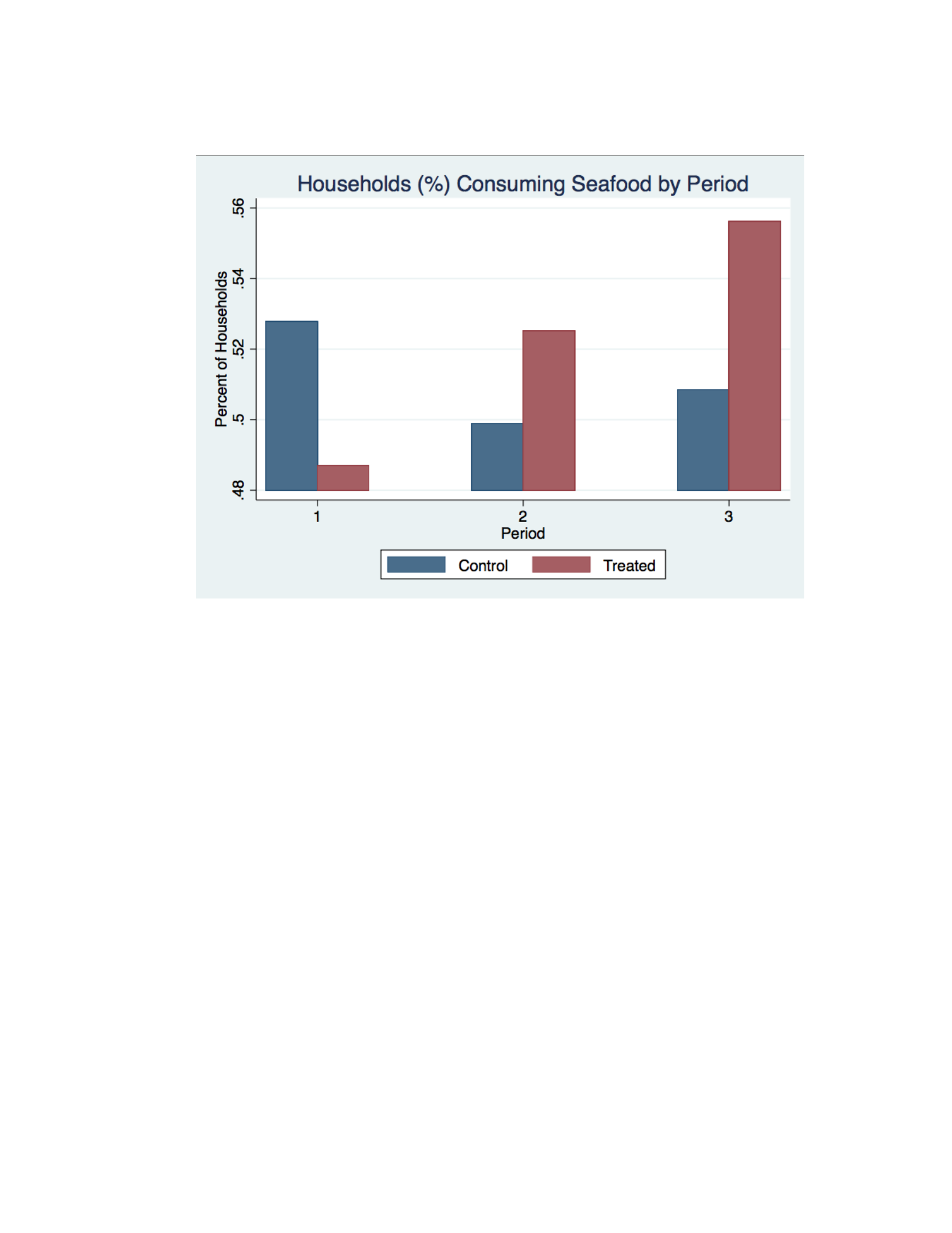
Figure 2.1: Effect of treatment on percent of households consuming any seafood by

period

Notes: Figure depicts the percentage of households that consumed seafood in the

previous week for control villages, in blue, and treated villages, in red, by period.

2. Location of Optimal Aid

2.1 Introduction and Motivation

‘Why do the poor stay poor?’ has been a long-standing question in the development

literature with important implications about how to best combat poverty. Poverty traps

occur when populations experience long-term chronic poverty with limited or nonexistent

opportunities to accumulate wealth. These systems are characterized by self-reinforcing

mechanisms causing poverty to persist (Azariadis and Stachurski, 2005). The most useful

application of poverty trap models occurs when there exist multiple long term equilibria

separated by a critical asset threshold, called a “Micawber Threshold” (MT), which is an

unstable dynamic equilibrium separating the basins of attraction of the high and low

wealth equilibria (Zimmerman and Carter, 2003; Carter and Barrett, 2006). This specific

type of poverty trap is known as a multiple equilibrium poverty trap where households

with initial wealth above the MT tend to experience a growth in wealth and approach the

high-wealth equilibrium, while households just below the MT get mired in poverty.

Poverty trap models are useful in explaining why some groups appear to be stuck in

chronic poverty while apparently similar groups prosper by highlighting how small initial

differences in wealth can dramatically affect long term wellbeing, which has important

policy implications.

It is possible short-term aid can change long term wealth trajectories by setting

households on a path of wealth accumulation towards a high wealth equilibrium rather

than the household falling further into poverty. In the theoretically deterministic setting

where random shocks to wealth are assumed away, providing aid just above the MT

ensures a household will progress towards the high-wealth equilibrium and would be the

ideal location to target aid policies (Barrett 2005). However, if aid falls short of the MT,

the impact of aid will be short-lived with household wealth diminishing overtime,

approaching a low wealth equilibrium. In this paper, we addresses whether targeting aid

at the MT is optimal when wealth generation has a stochastic component.

While poverty traps have recently received a large amount of attention, too little

work has been done to analyze how to optimally provide aid to those stuck in poverty

traps. There has been some work analyzing how well subsidized insurance programs

perform at reducing poverty for populations experiencing or vulnerable to multiple

equilibrium poverty traps. Janzen et al. (2012) look at a pastoralist system in Northern

Kenya3 and find those closest to the MT would benefit most from insurance, as even a

small downward shock to their productive assets (in this case the loss of an animal) may

put the household on a trajectory of further herd loss and potentially resulting in exiting

from pastoralism altogether. However, it is also this group who are least likely to

purchase insurance due to the high opportunity cost for households around this critical

wealth level. For these vulnerable households, selling an animal to pay for insurance may

put them below the MT and would place them on the unfavorable negative trajectory.

The authors suggest subsidized insurance, especially targeted at the vulnerable

households, may prove a promising means of social protection. Similarly, Kovacevic and

Pflug (2011) show fair insurance is only effective at reducing the risk of experiencing a

poverty trap for wealthier households in theoretic setting. The authors use a ruin theory

model where once a low-level wealth threshold is crossed, escape from poverty becomes

impossible, and model wealth as a having deterministic growth with low-probability, but

3 This is a highly studied socioeconomic system for poverty traps, which we discuss in

more detail later.

severe downward shocks. The authors show only wealthy households can benefit from

insurance, while the most vulnerable households cannot afford the cost of insuring

against downside risk even though they have the highest benefit of insurance. These

studies suggest while insurance may be included in an overarching poverty reduction

strategy, alternative forms of aid are necessary to help the most vulnerable segments of

the population when a potential poverty trap is present. The insurance literature

concerning poverty traps has mostly addressed fair insurance, where the burden of

purchasing insurance falls on the recipients. This can be thought of as a tool for

eliminating poverty rather than aid, where the cost of assistance is borne by external

agents such as charitable donations or taxation on other members of the society.

Barrett (2005) makes a distinction between two general policies: ‘cargo nets’

are policies to lift people up to a certain wealth level and ‘safety nets’ to prevent people

from falling below it in the future. Some examples of safety nets are emergency feeding

programs and disaster relief; additionally heavily subsidized or free insurance would be a

form of a safety net. Cargo nets are designed to create pathways out of poverty and can

be in the form of direct transfers (in the form of cash or productive input) or alterations to

the socio-economic system such as land reform, school feeding programs, subsidized

farming inputs, and targeted microfinance (Barrett, 2005). In practice, the form of the

cargo and safety net may impact the effectiveness and care must be placed to determine

the appropriate form of aid depending on the context. For our purposes, we assume cargo

nets and safety nets having the same effect regardless of the specific form they take and

for the remainder of the paper, we will be treating a cargo net as a direct transfer and a

safety net as free insurance at a specified wealth level.

While it is useful to think in these terms, little has been done to understand what

types of policies work best to combat poverty traps as well as what wealth level these aid

policies should target. Ikegami et al. (2016) provide a good start to compare the

theoretical effectiveness of safety nets versus cargo nets by comparing the long run

effectiveness of two aid strategies; a needs based aid policy, composed of a cargo net

each period to lift the wealth of the poorest households as high as funds allow, and aid

targeted to individuals located nearest the MT to bring them up to the MT, essentially

providing a safety net at this level for those starting above the MT in the previous period

and a cargo net for some households starting below the MT. Under both policies, the aid

budget is funded by taxes imposed on the non-poor households in the population4. The

authors show large gains in long term poverty reduction by providing a safety net located

at the MT by effectively increasing the number of people who can sustain themselves at a

high wealth equilibrium and, hence, no longer require aid. While this work provides

substantial insight into optimal aid, the authors only test two policies and do not attempt

to identify where the targeted aid policy would be most effective, specifically would a

safety net placed slightly above or below the MT provide perform better than a safety net

at the MT. Additionally, as the authors point out, it is difficult to imagine an aid program

that provides aid to those at risk of falling into poverty while excluding those currently

suffering.

We focus on a policy of providing a minimum level of wealth, similar to the

needs based aid strategy in Ikegami et al. (2016). However, we focus on identifying the

4 An important implication of this is the total aid budget increases as poverty is reduced

due to increased proportion of the population being taxed, which partially drives their

results. While this assumption is not unreasonable, the authors’ results may not apply to

cases where a large portion of the aid budget comes from foreign aid.

optimal level of aid to provide in the face of poverty traps. Currently there is no

consensus of where an optimal safety net would lie in relation to a Micawber Threshold.

Barrett (2005) suggests for safety nets to be effective, they must be set above the

Micawber Threshold, which is certainly true for the deterministic case. However,

Plucinski, Ngonghala, and Bonds (2011) show safety nets set below critical thresholds

can lead to long term escape from disease-driven poverty traps, a specific cause of the

poverty trap we discuss in the next section, using numerical simulation. It is important to

note, Plucinski, Ngonghala, and Bonds (2011) define ‘safety net’ as a policy bringing

individuals up to a minimum level and ensuring they do not fall below it in the future,

similar to the policy we consider. This is analogous to a combination of a ‘cargo net’ and

a ‘safety net’ in Barrett’s (2005) terminology and is analogous to the needs based strategy

used by Ikegami et al. (2016). Plucinski, Ngonghala, and Bonds (2011) show high level

of wellbeing is possible even when aid is provided below the MT, but do not attempt to

prove this is optimal, leaving the question of the optimal level of aid unanswered. We

seek to fill this gap using numeric simulation to test the effectiveness of aid across a wide

range of aid levels to determine where the optimal aid level is located in relation to the

MT. We find the MT for a basic wealth policy with the optimal aid level usually falling

about 2-3% above the MT. We find the optimal aid is predominately determined by the

cost of poverty reduction and the level of poverty reduction is a secondary concern. This

arises due to the formation of an ‘aid trap’, where there is a region below the Mcawber

Threshold where both the cost of reducing poverty and the amount of poverty can both be

reduced. We show this occurs because the cost of providing aid actually decreases as the

level of aid increases for some range of aid levels below the Micawber Threshold. This is

the point where aid begins to lift people out of poverty allowing them to no longer be

dependent on the safety net.

An aid trap is used to describe the situation where some populations appear to

become dependent on external aid to maintain wealth levels. Typically, aid dependency is

used to describe when an individual, household, or community cannot meet its basic

needs without external aid (Lentz et al., 2005). This dependence may come about by

households relying on safety nets rather than taking the necessary steps to self-protect

themselves from downside risk, known as the moral hazard problem, potentially even

resulting in reducing work hours or exiting the labor force entirely. For instance, Seleka

and Lekobane (2016) show government food rations reduce the likelihood of subsistence

farming for poor households in Botswana. Even without the moral hazard issue,

dependence makes providing aid less desirable, as there are no long-lasting benefits to

justify the cost of providing aid. However, if dependence is caused by aid failing to

surmount a MT, then there can be significant gains to aid so long as it is placed at the

correct level. This is similar to Rosenstein-Rodan (1943)’s big-push theory to deal with

poverty traps at the macro level, which is there is a minimum level of resources that must

be devoted to an aid program if it is to have any chance of being successful.

Barrett and Carter (2013) motivate the importance of understanding the

underlying structure of the poverty to determine the appropriate aid to combat it. If a

multiple equilibrium poverty trap exists, identifying the existence and location of MT is

critical to achieve long-term lasting gains in welfare from aid policy. We show how an

aid trap can occur when providing aid to those stuck in a multiple equilibrium poverty

trap and show costs can be reduced by increasing the level of aid above the MT to put

households on a path of wealth growth and eventual exit from poverty. This reduces the

dependency on external aid, resulting in a lower cost of providing aid. We use this

observation to introduce a new twist on the aid trap and define the inefficient aid trap,

which occurs when both the cost of aid and the levels of poverty can both be reduced.

Thus, the aid policy is inefficient as there is a clearly superior aid policy available. The

inefficient aid trap is particularly useful when discussing the location of optimal aid and

we show the upper bound of the inefficient aid trap is the lower bound of where optimal

aid can occur.

This paper seeks to enhance our understanding of how to combat poverty traps by

identifying the aid trap caused by providing too little aid and determining the relationship

between the optimal aid level and the MT. We show the cost of providing aid largely

determines the location of optimal aid. We use this to find the local minimum for the cost

of providing aid and find it occurs slightly above the MT. Thus, optimal aid must either

be close to non-existent or set above the MT, consistent with Barrett (2005). We use this

minimum aid level to identify the inefficient poverty trap caused, in part, by the

increasing costs as level of aid decreases from this point, due to increased number of

impoverished people being supported by the safety net. Additionally, we use the shape of

the cost curve to show when there is uncertainty concerning the location of the Micawber

Threshold and the location of optimal aid, it is better to err on setting aid too high. This

occurs because the slope of the cost of providing aid is extremely steep just below the

MT, which results in a large penalty for providing aid too low, even if its only by a

relatively small amount. Together the results from this chapter provide a theoretic

foundation, which can be built upon to inform aid policy decisions when a multiple

equilibrium poverty trap is identified.

2.2 Poverty Trap Background

To begin the discussion of poverty traps, it is useful to distinguish between different

types of poverty as well as measures of poverty. Not all poverty is created equal, as the

duration of poverty may be just as important, if not more so, than the severity of it. Some

people who are currently poor may not be expected to be poor in future periods, or vice-

versa. While it is usually more convenient to take a snapshot of wealth levels in a given

period to define who is poor and who is not, such as the commonly used Foster-Greer-

Thorbeke (FGT) measures, the poverty trap literature focuses on the importance of

identifying the structural nature of poverty to provide a forward-looking measure to

distinguish if a household is likely to be poor in the future. Carter and Barrett (2006)

provide a detailed look at how poverty measures have evolved over time and advocate for

using asset-based poverty measures, opposed to those based on consumption or income,

as these measures capture the dependence of future wellbeing on current levels of

productive assets. Assets causal relationship with future wellbeing is a critical component

of the poverty trap literature with strong theoretic and empirical foundations and useful

for distinguishing between stochastic and structural poverty.

Carter and May (2001) introduce the asset poverty line to distinguish between

structural/chronic and transitory/stochastic poverty. Stochastic poverty is when a

household has a low level of consumption/income in a period, and is hence poor as

defined by traditional poverty measures, but is unlikely to remain so in the future due to a

large asset base. Structural poverty is when a household has a low-level of productive

assets, which would predict a low level of wellbeing in future periods. The asset poverty

line is the level of assets at which expected income in the future is equal to the income

poverty line. This largely began the transition into focusing on productive assets opposed

to income/expenditure measures, which are far more stochastic and less predictive of

future wellbeing. The asset poverty line still has the disadvantage of being rather

arbitrary. Individuals’ with wealth on either sign of this assigned threshold have nearly

identical levels of wellbeing, however one is defined as poor while the other is not.

Another downside to using assets, as a wealth measure is it can be difficult to

aggregate assets into a usable measure (Carter and May, 2001; Carter and Barrett, 2006),

especially since each livelihood will depend on different assets to produce wealth. Even

when just considering one livelihood, it may be difficult to determine the relative value of

a given productive asset, which may be complicated if certain assets become more

productive when owned together, for instance while a plow and an ox each provide some

level of productivity to a farmer individually, a plow becomes more productive when

paired with an ox to pull it. The more complicated the socio-economic system, the more

difficult asset aggregation becomes, which adds to the empirical complications of using

asset-based measures (Barrett and Carter, 2013). However, the advantages of productive

assets deterministic relationship with future wellbeing still make asset-based poverty

measures desirable even with the additional empirical challenge of creating an asset

measure.

Carter and May (2001)’s asset measure is still a static way of measuring

wellbeing and suffers from not being able to consider potentially predictable changes in

assets over time and focuses on some arbitrary asset poverty line. This is improved upon

by Carter and Barrett (2006) who introduce the idea of the asset-based MT, which is a

forward-looking measure focused on how assets are likely to change over time and

whether this will result in poverty, in terms of income/expenditure, in the future. The MT

separates where productive assets are expected to grow over time or diminish to a lower

level making it a dynamic measure of poverty. Those with assets above the MT are said

to be structurally non-poor, regardless of income/expenditure in any current period.

Understanding the structure of poverty is essential to determine the amount and

type of aid that can effectively allow households to escape poverty. There are a number

ways in which a household can experience poverty and, depending on the form, may

require different forms of aid to overcome it (Barrett, 2005). Transitory/stochastic, or

short-term, poverty occurs due to the randomness inherent in wealth dynamics. A

household, which is typically not impoverished, may fall below a poverty line, however

defined, in a period due to a negative shock, but if the household’s underlying

circumstances have not changed, e.g. there is no change in their productive assets, the

household will likely exit poverty in later periods (Carter and Barrett 2006). While not

desirable, transitory poverty does not require external aid to fix, as households will

recover from shocks over time and progress out of poverty. Providing short-term aid (e.g.

food aid in response to drought) will be effective in reducing short-term reduction in

wellbeing following negative shocks and should be focused on speeding the recovery

process (Nashold, 2013).

Structural, or chronic, poverty is characterized by long spells of low wellbeing

where once a household becomes poor it is likely to persist, perhaps even generations.

Structural poverty occurs when a household has a low level of productive assets that are

not growing, or expected to grow, over time and this level of assets cannot produce the

income/expenditure required to surmount an income/expenditure poverty line. The

poverty trap literature breaks chronic poverty down into two categories: single

equilibrium and multiple equilibrium poverty traps. Single equilibrium poverty traps

describe a situation where the socio-economic circumstances will always push

households towards some low-level of well being below a poverty line. Regardless of

initial asset endowments, overtime households will be pulled into poverty absent external

aid. Providing aid can yield short-term improvements, but will have no long-term impact

on wellbeing unless the socio-economic conditions underpinning the poverty trap are

changed. In this system, meaningful aid must be long-term without any expectation of

eliminating the poverty (Hubbard and Duggan, 2009; Ikegami et al., 2016). The single

equilibrium poverty trap is extremely rare if not non-existent, as it is hard to imagine a

form of poverty where there is no amount of aid could change the long-term wellbeing of

those in the system. However, if the amount needed to escape poverty is large enough, it

may be appropriate to model the poverty as a single equilibrium poverty trap.

We follow the majority of the poverty trap literature and focus on the multiple

equilibrium poverty trap where small differences in wealth can result in dramatically

different long-term outcomes depending on which side of the MT one falls. This point

becomes especially important when considering the implications of downward shocks

such as natural disasters. If for instance a flood, drought or hurricane destroy productive

assets, the primary means of storing wealth in many developing contexts where

functioning credit markets are not present, this could dramatically alter the future

wellbeing of the household. Where the household was once able to sustain or grow

wealth, if a shock drops wealth below the MT, the household will be on a wealth

trajectory where long-term poverty may be inevitable without external assistance. This

provides strong motivation for aid policies to prevent households from falling below the

MT, in Barrett (2005) terminology, providing a safety net around the MT to keep

households on high-wealth trajectory.

In general, multiple equilibrium poverty traps are caused by non-convexities in

wealth accumulation or an ‘S’ shaped relationship of income/asset dynamics. These can

occur at any scale from countries down to individuals with the potential for poverty traps

at different scales to occur simultaneously and reinforce each other (Barrett and Swallow,

2006). Barrett and Carter (2013) provide a detailed description of what can cause the

non-convexities in asset accumulation, which underpin the multiple equilibrium poverty

trap at the different scales. We focus on the micro-scale and summarize some of the

mechanisms, which, in theory, cause multiple equilibrium poverty traps at the individual

or household level.

One largely studied cause of the multiple equilibrium poverty trap centers on

physical work capacity, which declines more rapidly when wealth drops below a critical

level (e.g. Dasgupta and Ray, 1986). In this example, malnutrition leads to lower

productivity resulting in lower incomes, which in turn exacerbate the malnutrition. This

self-reinforcing mechanism ensures once the Micawber Threshold is crossed the

individual will fall deeper into poverty. A closely related set of literature focuses on how

disease reduces work capacity. Plucinski et al. (2011), among others, consider the case

where disease prevalence is inversely related to wealth levels, that is, poorer individuals

have less access to healthcare and get sick more often and/or recover from sickness more

slowly. Once an individual becomes sick, their earnings decrease, which is intensified the

longer they are sick. This is an example of a poverty trap with multiple and non-separable

assets, health and wealth. The interaction of the two can result in a tipping point, where

once poor individuals becomes sick, they become stuck in a disease driven poverty trap.

The non-tradability of health, i.e. you cannot lend someone your good health or borrow

against it in the future, is a central feature to other causes of poverty traps as well.

Another largely studied case concerns natural resource degradation. The

productive capital in natural resources behaves similarly to health in the nutrition or

disease driven poverty trap models, where it is largely not tradable. The typical case here

occurs where farmers below a certain wealth level cannot afford fertilizer, which lowers

the productive capacity of farmland overtime (Antle et al., 2006; Stephens et al., 2012).

With slightly larger initial asset endowments, farmers could invest in fertilizer. This

maintains or increases farm productivity eventually resulting in further investment in

assets and a higher standard of living.

Multiple equilibrium poverty traps can also be caused by increasing returns to

scale over some wealth range caused by multiple production technologies with varying

levels of fixed costs. If a more productive livelihood requires an expensive input, a

household must have an initial endowment of wealth to purchase it before it has access to

the increased level of production (Carter and Barrett, 2006; Ikegami et al., 2016). One

largely studied case of multiple production technologies is the pastoralist system of

Eastern and Southern Africa, where a minimum herd size is required to engage in the

more productive mobile pastoralism (e.g. McPeak and Barrett, 2001; Lybbert et al., 2004;

Toth, 2014), which we describe in more detail later in this section.

A necessary feature in all of these is some inability to borrow against the future in

order to surmount thresholds. This could be due to the nature of the asset, such as health

or, more typically, due to a lack of functioning credit markets. When credit is freely

available, individuals could surmount the MT and pay off the debt with the increased

returns from the high production technology. However, many impoverished populations

especially in remote rural areas do not have access to formal credit markets (Besley,

1995; Jacoby and Skoufias, 1997). Barrett and Carter (2013) suggest the most likely

cause of multiple equilibrium poverty traps would be some increasing returns to scale in

production over some level, such as different production technologies with varying levels

of fixed costs, combined with lack of financial markets preventing households from

borrowing to switch to a more profitable production technology. Most of the underlying

causes of the multiple equilibrium poverty traps share the same fundamental behaviors.

Thus, while the theory we present in the next section is presented as a poverty trap caused

by multiple production technologies, the results can be applied to other causes as well.

The main exception occurs poverty traps are caused by the interaction of wealth and other

asset stocks, such health or local natural resources, where the poverty trap must be

defined in multiple asset space. This complexity is left for future work where a more

complex model allowing for the interaction of multiple assets is allowed for. This model

can then be compared to our basic model to determine how this complexity impacts

results.

The theory of poverty traps has been applied to a diverse set of applications and

used to motivate development policy at scales from the micro to macro level. However,

there has been long standing difficulty in empirically identifying multiple equilibrium

poverty traps, even in contexts where theory would predict them to occur. Specifically, it

is difficult to identify the existence and location of Micawber Thresholds. While many

empirical studies have failed to identify poverty traps, this does not prove poverty traps

do not exist, but merely testing for non-convexities in asset accumulation has many issues

including significant measurement error, lack of observations occurring near non-

convexity, and non-random attrition to name a few, which makes identifying poverty

traps extremely difficult (Barrett and Carter, 2013; McKay and Perge, 2013; Kraay and

McKenzie, 2014). Additionally, thresholds may be heterogeneous based on ability level

(e. g. Ikegami et al., 2016) or changing over time as socio-economic factors shift. We

provide a more detailed description of these issues and the empirical techniques used to

surmount them in section 4.

The existence of a multiple equilibrium poverty trap for any specific case is

inherently an empirical question, which we do not seek to answer here, but rather extend

our knowledge of how to provide aid in situations where they are found to arise. We

abstract away from many of the empirical challenges and consider the case where a

poverty trap exists and, importantly, know the location of the MT to determine whether

aid should be targeted at this dynamic wealth threshold to provide the foundation for

future aid policy decisions. While the model we present in section 3.3 is intended to be as

general enough to be applied to many contexts where multiple equilibrium poverty traps

exist, it is helpful to couch some of the discussion in terms of a specific context. We

briefly discuss one notable economic system where multiple equilibrium poverty traps

have been identified and much of the poverty trap literature has been focused; the

pastoralist system eastern and southern Africa.

We follow a large portion of the poverty trap literature and focus on the mobile

pastoral system of the arid and semi-arid lands (ASAL) of east and southern Africa. The

ASAL is characterized by bi-annual dry seasons with frequent occurrences of severe

drought making traditional farming largely unproductive making pastoralism the main

livelihood for this region. This system provides an ideal context for studying poverty

traps, in part, due to access very limited economic outside of pastoralism and a single

productive asset, the herd, is the main form of wealth. With only one main productive

asset, we can circumvent the many issues associated with asset aggregation (Carter and

Barrett, 2006). Additionally, this economic system is comprised largely of two groups of

households, those with large herds engage in mobile pastoralism, moving to different

water sources and grazing lands, and households with small or non-existent herds who

are forced into sedentarism.

Several studies have empirically identified poverty traps in this system, which

arises due to requiring a large enough herd size to engage in mobile pastoralism (McPeak

and Barrett, 2001; Lybbert et al., 2004; Toth, 2014). These papers identify a Micawber

Threshold in herd size, below which herd size tends to decrease, in other words

productive assets decrease, eventually resulting in the far less productive sedentary

pastoralism and, sometimes, exiting from pastoralism altogether (Little et al., 2008).

Mobile pastoralism represents a more productive production technology by providing

access to additional grazing and watering areas. In this context, mobile pastoralism is

only possible when the herd is large enough to support the pastoralists, consuming meat,

milk and blood from the herd itself while moving between watering holes and grazing

areas. When a herd becomes too small, households are forced to stay near the village

which limits access to water (McPeak and Barrett 2001) and grazing lands resulting in

further loss of animals largely due to overexploited grazing lands near these villages due

to overstocking (Santos and Barrett 2011). This is an ideal example of the multiple

production technologies causing a non-convexity in asset accumulation.

There is strong evidence people perceive and respond to the existence of

Micawber Thresholds. Hoddinott (2006) surveyed farmers in rural Zimbabwe, who report

requiring at least two cows/heifers to maintain a stable herd size, which is consistent with

Hoddinott and Kinsey’s (2003) finding farm incomes in the area rise when farmers own

at least two cows. In the ASAL context, Santos and Barrett (2006) surveyed of the

Ethiopian pastoralists who report a critical herd size consistent with empirical findings of

Lybbert et al. (2004) of minimum herd size of about 4 TLU per person to engage in

mobile pastoralism. There is also mounting evidence of behavioral responses of

households, which would only be optimal if the household had assets around a perceived

MT. One behavior is ‘asset smoothing’ where household’s around a MT tend to forgo

consumption rather than reduce productive assets (either through selling or direct

consumption of livestock) when faced with negative shocks (Zimmerman and Carter,

2003; Carter and Lybbert, 2012). This behavior is in opposition to the typical economic

prediction of ‘consumption smoothing’ proposed by Deaton (1991), which predicts

households maximize their inter-temporal utility by maintaining relatively consistent

consumption, even when faced with negative income shocks. Observing asset smoothing

for some range of the population with consumption smoothing for the remainder of the

population is a strong indicator of non-convex asset accumulation with a MT in the

vicinity of where households’ are asset smoothing. Relatedly, we can also observed risk

taking behavior just below a MT. While typically households are risk-averse, that is they

prefer lower levels of risk, households just below the MT may gamble on riskier

production technologies/behaviors in the hopes of a positive stochastic outcome allowing

them to surmount the critical asset threshold (Lybbert and Barrett, 2011). Together these

studies make a strong case households are aware of the existence and location of MT

when a multiple equilibrium poverty trap exists.

This begs the question, if households know the location of MT, why can’t they

engage in alternative behaviors to surmount this threshold? A clear example in the mobile

pastoralism context is if mobile pastoralism is more productive, but requires a minimum

herd size; why don’t household’s with small herds pool their herds, or lend their herd to a

household with a large herd, in order to surmount this threshold? The practice of herd

aggregation, or professional herders, is more common in western Africa (Swift, 1986),

but in the ASAL of eastern and southern Africa the shorter more frequent migrations

decrease supervision cost, which increases the cost of reciprocal herd sharing (Santos and

Barrett, 2011; Toth, 2014). However, we do see some communal coping mechanisms.

Informal insurance exists in many locations of rural Africa where neighbors and relatives

give productive assets or food items to households who experience large negative shocks,

such as livestock death. In eastern Ethiopia, a system of informal insurance based

partially on the charitable obligation inherent in the Islamic religion as well as a form of

self-insurance due to expectations of reciprocity in the future (Devereux, 2006; Beyene,

2013). However, this is not always the case. For instance in rural Tanzania, informal

insurance networks are uncommon present even though these socio-economic

environments appear very similar (Amani et al., 1987; Dercon, 1998). Even where

informal insurance is present, systematic shocks that are frequent and/or severe reduce

the likelihood of the success of this type of informal insurance (Beyene, 2013). There

does appear to be a lack of mechanisms to deal with the multiple equilibrium poverty

traps within the community, motivating the need for external aid. In the following section

we present our poverty trap model, which we use to analyze how to best provide this aid.

2.3 Poverty Trap Model

Poverty traps are an inherently dynamic method of looking at poverty, which focuses on

how wealth, measured in some aggregation of productive assets, changes over time.

While identifying an appropriate wealth measure has its own empirical challenges, which

depends heavily on the socio-economic context of the system being studied, our model

assumes household wealth is knowable and incorporates all meaningful productive assets

making it the sole predictor of future wealth, apart from a stochastic component. We

model wealth growth using a transition function with two production technologies, which

implicitly incorporates consumption/saving decisions and optimal behavioral responses.

This simplification allows us to circumvent specifying and including an intertemporal

utility function to govern wealth dynamics through consumption and savings decisions,

which would obscure results due to added complexity. A more complete model should

include a utility function to explicitly allow for optimal behavioral responses when facing

a poverty trap, most notably asset and consumption smoothing (see Zimmerman and

Carter, 2003; Hoddinott, 2006; Carter and Lybbert, 2012), but we save this for future

research. Additionally, we assume there is no access to financial markets so households

are not able to borrow to overcome the Micawber Threshold, which is consistent with

many of the locations where poverty traps have been identified, most notably the

pastoralist system of the ASAL of East Africa (e.g. McPeak and Barrett, 2001; Lybbert et

al., 2004; Toth, 2014).

Multiple equilibrium poverty traps have two or more dynamic wealth equilibria,

with at least one of those falling below a poverty line, however defined. For simplicity,

we consider a dual equilibrium poverty trap where there exist two stable dynamic

equilibria for assets separated by an unstable dynamic equilibrium, the Micawber

Threshold, which we label M. Households choose the production technology, which

maximizes wealth in the next period based on the households’ current wealth level. For a

given wealth, w, at time, t , we model the transition function for a household as:



T (w )



max(a w  b )





t 1









{L, H}

where



is the production technology, which takes values L and H, representing low and

high level production technology respectively. a and c are scaling and curvature

parameters for their respective and b represents the fixed cost of production technology

where the high production technology has some positive fixed cost and the low

production technology as has no fixed cost, ensuring wealth growth is strictly possitive,



and bH 0. Additional constraints on the parameters: 0 aL aH

and







with no restriction on the relationship between cL and cH . Alternatively, this can be

written as:

where is the switching point between technologies, which occurs when

(a w)



(a w  bH )

H .5 When a

ssets

are above , the high production technology

will

generate more assets than the low production technology and vice versa. For a multiple

equilibrium poverty trap to exist, assets must have a negative expected growth rate at the

technology switching point, . This yields one unstable dynamic equilibrium at

M and two stable dynamic equilibria, w* and w* , corresponding to where the low and

L H

high dynamic equilibria for the low and high technology respectively. Over time,

households with assets starting above M will approach w* and those with initial assets

below M will approach

. If

, the transition function would exhibit positive

growth until w* is reached, with w* being a unique dynamic equilibrium.

Figure 3.1 depicts an example where individual production technologies result in

a multiple equilibrium poverty trap. The low production technology is depicted in black

and the high production technology in blue. The 45-degree line, shown in red, can be

interpreted as where wealth in the next period equals weatlh in the current period.

Anywhere the transition function intersectst the 45-degree line represents a dynamic

equilibrium with stable equilibria being those that cross from above. Figure 3.1 depicts

the two stable equilibria for the high and low production technologies respectively.

Anywhere where the transistion function lies above the 45-degree line will result in asset

growth and when the transition function lies below the 45-degree line, assets will decline

5 Note the time subscript is removed here, as the technology switching point is time

invariant.

over time. We see lies below the 45-degree line, a requirement for the multiple

equilibrium poverty trap to exist.

Figure 3.2 shows the transition function composed from the individual production

technologies depicted in Figure 3.1. It shows the transition function is comprised of the

maximum of the two separate production functions. Additionally Figure 3.2 includes the

Micawber Threshold. As we can see it occurs where the transition function intersects the

45-degree line from below, indicating an unstable equilibrium. Wealth above M will be

in the basin of attraction of the high wealth equilibrium, w* , and will approach w* over

H H

time while those below M will trend towards w* .

We also introduce an asset poverty line, z, which represents the level of

productive assets that produce the amount of income/consumption equal to the more

typeical income/consumption poverty line, on average. Any individual with wealth below

z in a period can be said to be impoverished acording to this static measure. To

distibguish between structural and transitory poverty we also need to look at the

Micawber Threshold. As we described in the previous section, the Micawber Threshold

represents a dynamic asset poverty line. Everyone with wealth below M are said to be

structurally poor regardless of whether current assets are below an asset poverty line.

When houshold wealth is below z and M, the household is structurally and chronically

poor and when household wealth is above both z and M the household is non-poor.

However, when wealth falls between the two poveryt measures, we see households which

may be strucutrally poor, but currently non-poor or just in transitory poverty and will

eventually emerge from it. Figure 3.3 depicts a scenario where z M , which depicts the

case where there exists some transitory poverty. When M w z, the household is

currently poor as assets are below the asset poverty line, but structurally non-poor as

assets will increase over time resulting in an exit from poverty. Figure 3.4 shows the case

where M z . When z w M , the household is structurally poor, even though current

assets are temporarilly above the asset poverty line, in other words the household is

transitorilly non-poor. This highlights the importance of using the benefit of using the

Micawber Threshold opposed to static poverty lines, however, in our analysis we utilize

more typical poverty measures, some of which depend on the asset poverty line.

We introduce randomness into the model as lognormal error, independent of

production technology. A more realistic model would allow each production technology

to have systematically different error components; for instance, McPeak and Barrett

(2001) show pastoralists in the ASAL of eastern Kenya experience greater risk of animal

loss due to raiding6 the further away from towns they graze, which would be

systematically higher variance for the high production technology. We do not allow for

technology dependent stochasticity, as it would complicate the decision of when to

switch between technologies without substantially altering the fundamentals of the

system. Thus, our stochastic model can be written:



max(a w  b )





t 1



where 2 is the process variance. The lognormal error ensures the stochastic component

is tied to wealth level ensuring shocks have a proportional impact on households, for

example a drought would be better modeled as killing off a percentage of a herd rather

than a given number of animals, which is also consistent with much of the financial

literature models how financial assets (stocks, derivatives etc.) evolve over time. Other

poverty trap models have modeled randomness as some negative shock, rather than

random error that can be positive or negative (e.g. Ikegami et al. 2016), which is intuitive

to describe situations where drought kills off a large proportion of a herd with no real

reciprocal for a positive benefit. While our model does not lend as easily to this thought

process; functionally, it works the same. The main difference is our transition function is

centered at the median7 of the distribution, rather than the maximum of the distribution.

We feel this provides a more meaningful interpretation of the high and low equilibria and

the MT while still capturing the dynamics of the poverty trap. With these underlying

wealth dynamics, we introduce a social planner with the objective of reducing poverty

while still considering the cost of reducing poverty.

2.4 The Social Planner’s Problem

Rather than discuss optimal aid in terms of a as part of a government or aid organization,

which may have multiple, potentially conflicting objectives; it is useful to introduce the

abstract social planner with the sole purpose of determining the optimal level of aid to

provide to those stuck in poverty. We use the social planner to compare the costs and

benefits of providing aid. We can simplify this into two components: the cost of

providing aid and the social cost of poverty. Absent aid, there is no cost of providing aid,

however, the level of poverty is largest. Thus there exists a tradeoff between providing

7 It is the median, rather than the mean, of the distribution as we are dealing with

lognormal errors. The transition function in any given time period can be interpreted as

the in the





)

aid, with a monetary cost, versus the cost to society of having poverty. In this section, we

discuss how we model the social cost of poverty in terms of a dollar value, which we can

directly compare to the cost of providing aid, and use this to determine the total cost of

providing aid at varying levels. We show the optimal aid level is largely determined by

the cost of providing aid, which is decreasing just below the Micawber Threshold

resulting in a local minimum of the total cost of aid. Due to the shape of the cost of

providing aid, the cost of poverty becomes only a secondary consideration, suggesting aid

policy decisions can focus on costs of providing aid when combating the multiple

equilibrium poverty trap.

We model the social planner’s problem as minimizing the sum of two costs: the

cost of providing aid and the social cost of poverty. The social planner chooses aid level,

S , that guarantees a minimum wealth level for all households, which we call the basic

wealth policy. This policy is similar to the more familiar basic income policy, except the

guarantee is based on household assets rather than income. The present, or discounted,

cost of providing aid, c(S), is the sum of payouts to each household, i , in population, N

, with assets below the aid level to bring assets up to S at the end of each time period, t ,

summed over the length of the time horizon, T , with discount rate, . It is useful to

break cost of aid into two components: the initial cost of providing aid to bring

households’ assets up to S , which Barrett (2005) refers to as a ‘cargo net’, and the cost of

preventing households’ assets from falling below S in all future periods, called the

‘safety net’. Breaking it down in this way, we can write the cost of providing aid as:

N T N



c(S) (S  wi,0 )



 





T (w

i,t

| S)







1 i





i,t

| S



max[T (w

i,t



),S]

where

the + supe

rscript is

the shorthand notation,









max



x,0



Due

to the aid policy,

wealth is bounded at S , which is captured in the second equation. The first term is the

cost of the cargo net, paid in the initial period, t 0

, and the second term is the

discounted cost of the safety net for the duration of the policy. Breaking it down this way

allows us to estimate the cost of providing aid, which we describe in detail in chapters

four and five.

The social cost of poverty, C(P | S) , is a function of some poverty measure, P ,

which is partially determined by the level of aid, S .

C(P













where g is some weighting function capturing the negative impact of poverty, however

measured, and wt is the vector of wealth levels at time t. We do not explicitly include

any discounting function for poverty. Any discounting can be included in the function, g ,

or we can interpret the social planner as being indifferent between poverty today or in the

future.

In practice, the weighting function, g , will depend on a number of social factors

and captures how much a society dislikes poverty. We do not attempt to prescribe a

functional form of g , but we can make some standard assumptions about its form, which

intuitively hold across societies. The main feature we will rely on in our analysis is g is a

strictly positive function, as poverty is non-negative and has some social cost, which is

increasing with respect to poverty,





)



0 .

imply

ated, more poverty

wors

e for

P

society. For our analysis, we do not need to make any assumptions on the second

derivative of g , although, intuitively, the social cost of poverty is likely to be increasing





)





weakly faster as poverty becomes more extreme,



. While our results hold for

this extremely general form, for the remainder of the paper we will assume a functional

form of g to aid in the discussion and make the interpretations more accessible.

Specifically, we assume the social cost of poverty is a multiplicative transform of the

poverty measure:

g(P)







P ,

where  is some positive scalar capturing the cost of poverty. With this functional form,

the curvature of the social cost of poverty is largely determined by the poverty measure

itself and  acts as some scaling factor to transform the poverty measure into some

dollar value, which we can use to directly compare the cost of poverty with the cost of

providing aid. In other words, we assume the poverty measures themselves indicate social

preference over the cost of poverty; just not expressed as a dollar value, with lower levels

of a poverty measure correspond directly to a lower social cost of poverty.

The choice of poverty measure has important implications in many contexts as

each measure places weights on different aspects of poverty, such as amount of inequality

in society or the percent of the population below a defined poverty line. Some widely

used measures are the Gini coefficient and the Foster-Greer-Thorbeke (FGT) measures,

which we briefly discuss as well as show how each is calculated for a population in a

single time period. While typically these measures are based in expenditure or income,

Carter and Barrett (2006) show these measures can just as easily be applied to asset-based

wealth measures, consistent with our modeling framework.

The Gini coefficient is a measure of inequality rather than poverty, per se. It is a

measure of how wealth is dispersed across a population. It is calculated:

N N



| w





1 j







The coefficient can take on values between zero and one, assuming there is no negative

wealth. The larger the Gini coefficient, the higher the inequality of the system is. A Gini

coefficient of one means perfect inequality, where one individual has all the wealth, and

zero indicates perfect equality. A benefit of this measure is it does not rely upon an

arbitrary definition of poverty, such as the poverty line, like the members of the FGT

family. The major downside with this measure is it says nothing about the wellbeing of

households. A population where all households are mired in extreme poverty will score

well (a low value) using the Gini coefficient, while a population with high levels of

wealth with significant variability between households will score worse (a high value).

While the latter case is clearly preferable, it also has a more inequality, which highlights

why using the Gini coefficient by itself can be misleading. However, looking at the Gini

coefficient in conjunction with other measures that include some level of wealth or

wellbeing is useful.

The Foster-Greer-Thorbecke indices are a family of poverty measures sharing a

common functional form:

1 H  z  w  

FGT











 i 

 ,

i1

where  indicates the poverty measure, z is the asset poverty line, and H is the number

of households below the poverty line. The poverty headcount,  0, is the first measure

in the FGT family. It doesn’t put a weight on anything other than the number of

households falling below the poverty line and can be written:

FGT



H .

According to this metric, a starving household is just as undesirable as a household just

below the poverty line, which is not realistic. However, it can be used to look at the cost

of removing households from poverty, especially if one wants to consider the case of

eliminating poverty entirely or to bring percentage of households’ in poverty to some

level, which may be the objective of some government or aid program. A less severe

problem with all of the FGT measures is it does not give any weight to how households

above the poverty line. An extremely wealthy household with little to no risk of falling

into poverty is viewed as the same as a household just above the poverty line.

The second FGT measure is the poverty gap,  1, which is the difference

between a household’s wealth and the poverty line, summed across all households in the

population. This gives a measure of how impoverished the poor households are. This

measure partially weights inequality as poorer households have a larger weight. As with

all the FGT measures, it relies on an arbitrary poverty line and does not consider the

wellbeing of non-poor households.

How one measures poverty is important in many empirical contexts and can result

in different measurements of the severity of poverty as well as potential effects on

optimal aid strategies. For our analysis, we can circumvent the issue of selecting a

poverty measure by noting any poverty measure that depends solely on level of poverty

and inequality will have its own social cost function, g , which all behave similarly with

respect to S . Increasing S will have a positive effect on wealth levels and a negative

effect on inequality. For poverty measures that weight inequality, it is always as a

negative. Thus, increasing S has a positive benefit in terms of wealth and inequality

resulting in a lower level of poverty, however measured. Figure 3.5 depicts the

relationship between poverty measures as a function of aid level for one parameter

combination with an asset poverty line at w 70. We see the FGT measures equal zero

when aid level is set at or above the poverty line, as these measures only consider the

impoverished within the population. We see poverty is weakly decreasing for all

measures and we see significant drops in all measures slightly below the Micawber

Threshold.8 This drop corresponds to the aid level being high enough for individuals to

begin escaping poverty and holding themselves at the high wealth equilibrium, thus no

longer being dependent on the external aid. The measures which place a higher weight on

inequality exhibit a smoother decline, while the poverty headcount has little to no change

until a sharp drop. This is intuitive as lower levels of aid do not significantly impact the

likelihood of escaping poverty, but it does raise wealth levels for the most impoverished,

thus reducing inequality. All measures of poverty are weakly decreasing as aid increases.

This combined with our modest assumptions of g for our poverty measures, ensures the

social cost of poverty is decreasing as level of aid increases, g S 0 everywhere.

Because the poverty measures (and therefore the social cost) are weakly decreasing in

aid, the solution to minimum total cost ends up depending primarily on the cost function

for providing aid. We will demonstrate this feature of the problem more extensively

8 We do not include the Micawber Threshold in the figure as it clutters up the image and

is not the focus of the discussion here.

below, as it provides a compelling result: future applied researchers and policy makers

can focus almost exclusively on the cost of providing aid.

To show this, we start by modeling the social planner’s problem inclusive of the

social cost of poverty, as choosing the aid level that minimizes the sum of the cost of

providing aid and the social cost of poverty:

minc(S)



C(P | S)

We model this as an unconstrained optimization with the solution being the level of aid,

which is best for society, independent of available funds. In other words, we assume the

social planner has access to enough money. Adding a constraint does not fundamentally

change the nature of the problem, as cost of aid is explicitly included in the optimization.

Due to the poverty trap and the cost of aid being explicitly included, we do not find the

solution of the social planner’s problem to be an arbitrarily large S and we show later

optimal aid must either be close to non-existent (for the case of a society caring very little

about poverty) or located near the MT. We omit the non-negativity constraint on aid for

notational convenience; obviously, the choice set includes no aid.

Taking the first order condition of the social planner’s problem with respect to the

level of aid, we get:



c(S)





C(P | S)





c(S)





C(P | S) ,



intuitively, the optimal level of aid should balance the cost of providing aid with the

social cost of poverty. Aid should be provided up to the point where the marginal cost of

providing aid equals the marginal benefit of reducing poverty.

Intuitively, it may appear the location of optimal aid will depend largely on the

social cost of poverty. However, due to the underlying mechanics of the multiple

equilibrium poverty traps, we show the cost of providing aid is the primary concern for

our basic wealth policy and the social cost of poverty is a secondary concern, in terms of

where the optimal solution lies. Clearly, policy makers can choose no aid, which will

come at zero cost. Initially, for very low levels of aid, the cost of providing aid is strictly

increasing. Barring some edge cases (to be discussed below), if society values poverty

reduction sufficiently to take action, the optimal solution will be characterized by a local

minimum in the cost function for providing aid. We will show that this local minimum

will be at an aid level very close to the Micawber Threshold in nearly all cases where a

dual equilibrium poverty trap is the appropriate model. We will also show that this

phenomenon is driven by the structure of the poverty trap model. When the asset poverty

line, z, is below M, aid only up to z will result in (definitional9) poverty eradication but at

very high cost, so policy makers can keep poverty at zero but lower costs (and raise

wellbeing of those affected) by raising the aid level. On the other hand, when z is above

M, aid is only needed up to (a small interval above) the Micawber Threshold to propel

households to the high equilibrium. The supporting details for these claims are covered in

the next section.

The social planner’s problem is difficult to solve analytically so we turn to

numeric analysis to determine the optimal level of aid to combat the multiple-equilibrium

poverty trap. We input our model into MATLAB and simulate wealth paths for

9 When aid is set above the asset poverty line any measure such as the FGT poverty

measures, which measure poverty below the poverty line will equal zero. According to

these measures poverty will be completely eliminated, by definition.

households under varying levels of S to calculate the cost of providing aid as well as the

level of poverty. We start by generating wealth levels for 10,000 households using a

uniform distribution across relevant wealth ranges, 1 to 100, and simulated wealth

trajectories without aid for twenty periods. The 20th period we use as the starting wealth

levels, which approximates the steady state distribution resulting from the underlying

transition function. We then introduce varying aid levels of S and simulate wealth

trajectories for these households, which comprises our data. We vary high technology

parameters as well as discount rates and the maximum time period to generate data used

to determine what factors impact the cost of providing aid and the likelihood of poverty.

We do not vary the low-technology parameters for simplicity and ease of interpretation.

In previous iterations of this simulation we found the low-technology parameters did not

significantly impact our results as the high technology determines M and the

surrounding region, which largely determines the optimal aid level. For these data we

focus on the effect of the high technology parameters and include only a few levels of T

and



to show they do not play a significant role in determining the level of optimal aid

and aid levels and the inefficient aid trap.

2.5 Poverty Trap and Aid Mechanics

The total cost in the social planners problem is the sum of the cost of providing aid and

the social cost of poverty, which is the objective function we seek to minimize. The

lowest value of total cost represents what is preferred by society and depends on the cost

of reducing poverty as well as the social cost of poverty within the society. The social

cost of poverty depends on the level of poverty as well as the weighting function, ,

which translates a poverty measure into a dollar cost of poverty. The cost of providing aid

in the form of our basic wealth policy is the sum of the cargo net, to bring people up to

the desired aid level, and the present value of the safety net to keep people at this level in

all future periods, which depends on the number of people relying on aid and the

magnitude of the payouts each period. It is important to note the cost of providing aid is

independent of a specified poverty line – only the poverty measure itself is potentially

sensitive to the official poverty line. The basic wealth policy simply pays out to ensure

household wealth equals at least the aid level in each period and can be set anywhere in

relation to this poverty line. We can simulate the cost of providing aid and the level of

poverty and, hence, determine the social cost of poverty by assuming some value for the

weighting function , for each aid level. The sum of these components will be the total

cost, which the social planner is trying to minimize. In this section, we describe the

general form of these cost functions and detail some specific cases to motivate why we

can focus almost exclusively on the cost of providing aid for much of our analysis.

While the cargo net is strictly increasing with respect to aid level, the cost of the

safety net is decreasing over some range of aid level. This decrease is large enough to

cause the cost of aid to be decreasing over much of this range as well. Figure 3.6 depicts

these dynamics. The cost of providing aid, in black, is equal to the sum of the two blue

lines, the cost of safety net (solid blue) and the cost of the cargo net (dashed blue). This

comes about directly from how aid interacts with the poverty trap mechanics. Once

people escape the trap by crossing the Micawber Threshold, they are propelled to the

high wealth equilibrium and no longer need to be supported by the safety net. Reducing

the number of people supported by the safety net reduces the cost of providing a safety

net in each period, which in turn reduces the cost of providing aid. We show later this

drop in cost happens slightly before the Micawber Threshold. At this level of aid, we see

individuals being able to surmount the Micawber Threshold and propel themselves

towards the high wealth equilibrium. In addition, this level occurs around the technology

switching point, which represents where expected wealth change is most negative as

shown in Figure 3.6. Aid at this level typically represents the peak of the aid trap, where

payouts are large and the number of people supported is large. As aid increases from this

point, the expected payout per individual kept at the safety net decreases because the

expected wealth change is increasing (less negative) at this level.

Figure 3.7 depicts the typical relationship between cost of providing aid, in black,

and the likelihood of poverty, in blue. The x-axis is the level of aid, the left y-axis is the

present value of providing aid in terms of cost per person, and the right y-axis is the

percentage of the population below the poverty line, or the poverty headcount, over the

length of the simulation. We see at low aid levels, there is a minimal impact on poverty

level with costs rapidly increasing. Costs switch from increasing rapidly to sharply

decreasing around the technology switching point. This drop in cost is concurrent with a

sharp drop in the poverty level. This is intuitive, when the number of people being held

up by the safety net decrease, there will be lower costs each period. The shape of the cost

function is important. We see it is not strictly increasing with aid level creating a local

minimum of cost, which we call the minimum aid level,

. We later

show

Sˆ is the upper

bound of the inefficient aid trap.

The likelihood of poverty in figure 3.7 is expressed in its own scale, loosely

interpreted as the average amount impoverished household wealth levels are below the

poverty line, rather than in terms of a dollar value. We can transform this into its dollar

value by assuming a value for the weighting function, , so we are comparing the dollar

cost of providing basic wealth with the dollar cost of the level of poverty at all levels of

the safety net. The level of  determines how much society cares about poverty and can

significantly impact the optimal level of aid. Another important component, which can

impact optimal aid level, is the location of the poverty line. We consider three general

cases of how  and the poverty line effect the location of optimal aid: low value of 

and/or a low poverty line, a poverty line within the inefficient aid trap, and what we call

the typical case where  and the poverty line are sufficiently large. This last case is what

we focus much of our analysis on, as it is the most relevant to providing aid to those

stuck in poverty traps.

There are two cases where optimal aid will be close to nonexistent: when the

social cost of poverty is very low (a relatively small ) or when the poverty line is close

to the low equilibrium. The latter naturally requires a society using a poverty measure,

which depends on the defined poverty line such as any in the FGT family. It is easiest to

interpret our model in relative terms, rather than specific values. While we talk about

results in like terms, aka dollars, these are arbitrary units, which is meaningless without

the rest of the contest. For instance, saying the social cost of poverty is 75$ can mean two

very different things depending on whether to cost of providing aid is $1000 or $10. With

this in mind, the two cases both represent situations where poverty is relatively

unimportant to society. A low social cost of poverty indicates the cost of poverty

reduction is large compared to the benefits of removing poverty and a poverty line close

to the low equilibrium indicates the poverty trap results in only mild levels of poverty.

3.5.1. The Case of a Low Poverty Line

Figure 3.8 shows the case of a very low poverty line, which would affect the FGT

poverty measures, but not the Gini coefficient. The total cost function is expressed as a

solid black line, and is made up of its components, the cost of aid, the dash/dotted line,

and the social cost of poverty, the dashed line. We use the poverty gap to measure

poverty for this analysis. At low levels of aid, we see the total cost depends entirely on

the social cost of poverty, as the cost of providing aid is nonexistent at the low levels. We

see the cost of poverty is relatively low, as much of the population does not experience

poverty due to the relatively low poverty line. We see the total cost function has a local

maximum at the minimum aid level, which is simply the local minimum of the cost of

providing aid, but this does not correspond to the global minimum of the function. The

global minimum indicates the optimal aid policy, which occurs around the aid level 25.

3.5.2. The Case of a Low Social Cost of Poverty

Figure 3.9 shows a similar case of where the social cost of poverty is low, in other words

a low . We still see the local minimum of the cost of providing aid is not the global

minimum as the cost of poverty is always extremely small. Thus the optimal aid level in

this case is close to nonexistent, as the benefit of eradicating poverty is very small, since

society does not care much about it. Both cases have a global minimum of aid level very

low, as poverty is not a large concern in either case, resulting in a low level or non-

existent aid. These cases will have aid provided at a level below the start of the inefficient

aid trap. While these represent potential situations in the real world, they correspond to

situations where poverty is relatively unimportant making much of the discussion of aid

policy moot. Thus, we do not focus on this scenario for our analysis and focus on cases

where the poverty trap leads to substantial poverty, which society cares about enough to

eliminate.

3.5.3. A Poverty Line in the Region of the Aid Trap

A second notable case occurs when the poverty line lies within the inefficient aid trap.

When this occurs, the poverty measures which depend on the poverty line will all go to

zero sharply within the inefficient aid trap, making at least some of the range having a

zero cost of poverty. This results in optimal aid being exactly the minimum aid level, so

long as  is large enough. After the poverty line is reached, the total cost depends solely

on the cost of providing aid making the minimum of total cost be equal to the minimum

of the cost of providing aid.

First, some notation. In the context of our model, we define the inefficient aid trap

as including all levels of aid below

, for which the c

ost

of aid i

at lea

high a







. We denote a

0 the lower bound of thi

interval, for

hich c











, which

depicted in Figure 3.10. It is immediately clear from the Figure that the case of the low

poverty line (Section 3.5.1 above) is one in which z S0

. The beginning of the inefficient

aid trap occurs when cost first reach this level, which we label S0. We do not devote

much time to the S0 as it is not easy to empirically determine, it does not have a useful

economic interpretation nor is it particularly relevant for policy decisions.

Now

, consider the ca

ere







igure 3.11

shows

thi

wher

once again, the total cost is shown as the solid black line, the dot/dashed line is the cost of

providing aid and the dashed line is the social cost of poverty. We see after the cost of

poverty goes to zero, which occurs when aid level is higher than the poverty line, which

is set at 40 for this example, we see the total cost overlays the cost of providing aid, as

these are equal beyond this point. We see the local minimum, which is the minimum aid

level also is the global minimum. Thus, when the poverty measure used to value poverty

is in the FGT family and the poverty line lies within the inefficient aid level, the optimal

aid level lies exactly at the minimum aid level.

3.5.4. A Poverty Line above the Aid Trap

The last case occurs when the  is sufficiently large and either the poverty line lies

above the minimum aid level or we are using a poverty measure, which does not depend

on a poverty line, such as the Gini coefficient. For this case, the minimum aid level

becomes a lower bound for the optimal aid level. The exact location of optimal aid will

depend on , the slope of the poverty measure, and the slope of the cost of providing aid.

This is the case where the solution to the social planners problem holds, that is to say the

marginal benefit of reducing poverty equals the marginal cost of providing aid:

c(S)  C(P | S) .

S S

The other cases represent different corner solutions to the problem. Figure 3.8 depicts this

with the total cost being shown as the solid line, the cost of providing aid is the

dot/dashed line and the social cost of poverty is the dashed line. We see a global

minimum of the cost function occurs above the minimum aid level, which is why we treat

this as a lower bound. The solution to the social planners problem, that is to say the

location of the global minimum, occurs when the slope of the cost of providing aid equals

the absolute value of the slope of the social cost of poverty. This is the point where the

marginal benefit of eliminating poverty equals the marginal cost of providing aid. For aid

levels above this point, the cost of providing aid is increasing far more rapidly than the

cost of poverty is decreasing. This is consistent across poverty measures and under

different model parameters, and ensures the optimal aid level lies reasonably close to the

minimum aid level.

It is the structure of the dual-equilibrium poverty trap model that causes costs to

increase relatively faster than the poverty level drops at points above the Micawber

Threshold. It is for this reason that the minimum cost aid level is always so close to M,

and that the social planner can focus primarily on cost. Once aid is this high, the cost of

providing a safety net each period is relatively low. Increasing the level of aid does not

have much of an effect on the safety net cost each period, but has a large effect on the

initial cost of the cargo net. Thus increasing aid at points significantly above the

Micawber Threshold have larger costs due to the increased cost of the cargo net, without

a significant change in the likelihood of people falling below the aid level and having to

be supported by the safety net. Thus, poverty levels, however defined, do not change to a

large degree as safety nets rise beyond this point, but costs do increase significantly.

2.6 Does the Minimum Aid Level Approximate the Micawber Threshold?

We identify the upper bound of the inefficient aid trap by finding the minimum aid level,

, by identifying the local minima of the c

ost

function with respect to the aid level.

For

the vast majority of aid levels below this point, there will be a higher cost of providing

aid with a lower reduction in poverty, which comprises the rest of the inefficient aid trap.

Any aid set below Sˆ with a lower cost will have a non-noticeable impact on poverty

levels, which occurs at extremely low aid levels. While we cannot rule out the potential

the optimal aid level lies in this region, this would only be optimal if society has a very

low social cost of poverty, g , making the discussion of poverty reduction moot as

discussed in section 3.5. We focus on the relationship between M and Sˆ to determine

whether the Micawber Threshold should be the target level for aid policy.

Table 3.1 reports linear regression for the location of minimum aid, Sˆ . We find

M almost entirely predicts

regre

ssi

on coefficient around .99 for all model

specifications indicates Sˆ has almost a one to one relationship with M , which is

significant at the 1% level. We include the high equilibrium and sigma in alternative

models, which moderately improves the regression fit; both variables are equal at the 1%

level. We see our process variance parameter is has a positive effect on the location of

minimum aid, suggesting the more variance in the system, the larger the minimum aid

level should be.

Figure 3.13 shows the scatter plot with Sˆ on the y-axis and M on the x-axis as a

visual of this relationship. We include a 45-degree line to better visualize which side of

the MT the minimum aid level lies with observations to the left/above indicating the

Sˆ M . We see minimum aid level almost entirely lies above M . The only exceptions

occur when the Micawber Threshold is very close to the high wealth equilibrium, which

can be seen in figure 3.14. This occurs because the basin of attraction for the high wealth

equilibrium shrinks the closer the Micawber Threshold and the high wealth equilibrium,

in other words the equilibrium is less stable. Even if households reach this equilibrium,

the stochastic process is likely to drop them below it in the near future. This situation

would be better described as a single equilibrium poverty trap with some minor periods

of relatively high well being for the initially well endowed, or those who experience

repeated good luck, but this high wellbeing is short lived. We look closer at the

distribution of minimum aid levels for select parameters later in this section to get a

better estimate of how much larger Sˆ is than M .

We find the minimum aid level for our basic wealth policy lies slightly above the

MT. Rather than looking at the magnitudes of the MT and minimum cost when making

this comparison, it is helpful to consider the difference in percentage terms. Figure 3.11

shows the distribution of the percent difference between minimum cost and the MT as a

Sˆ



percentage of MT,



100

, under different

sets

of parameter

mulated 1000 time

Positive values are interpreted as how much larger the minimum cost of basic wealth is

larger than the MT, in percentage terms, with zero indicating the minimum cost is located

at the MT. We find the minimum aid level is, on average, 2-3% larger than the MT. The

spread of the distribution is largely determined by the process variance, 2 , with a larger

2 increasing the distance between the minimum cost level and the Micawber Threshold.

We also see larger shape parameters, aH and cH reduce the variability and lower the

distance. The distribution of minimum aid level lies fully above the MT, for these

parameter combinations as these parameters had a sufficiently large gap between the high



c(S

ˆ )



equilibrium and MT. Table 3.2 shows regression results of the effect of our parameters on

the percent difference. We see b and 2 have a positive effect on the percent

difference, while other parameters aH , cH and M all have negative effects. When the

multiple equilibrium poverty trap exists with a large enough basin of attraction around

the high equilibrium, we can interpret the Micawber Threshold as a lower bound for the

minimum aid level. As Sˆ is the upper bound of the inefficient aid trap, the Micawber

Threshold can be reasonably interpreted as this upper bound. We use this in conjunction

with comparing the slope of the cost curves on either side of Sˆ to suggest M should be

used as a lower bound for the optimal location of aid, without needing to specify a

functional form for the social cost of poverty, g .

Looking at the cost function around

see

osts

increa

e fa

ster below the

minimum aid level than above it,



, where the positive and negative

sign represent above and below respectively. This is an asymmetric penalty for

misspecifying the aid level, where there is a higher penalty, in terms of cost, to set aid too

low than too high. Since the level of poverty is decreasing with increasing aid, not only

does setting aid too low have a higher dollar cost, it also reduces the effectiveness of

reducing poverty. In the empirical setting there may be significant uncertainty in the

location of M and it may be impossible to determine

Due

to the a

ymmetric penalty,

these results would suggest placing an aid level above the estimated MT would be

desirable. This has the additional benefit of decreasing poverty to a larger degree while

still having a lower expected cost of aid.



c(S

ˆ )



Identifying the minimum aid level and the inefficient aid trap is one step short of

identifying the optimal aid level for a society, which depends on the social cost of

poverty g . However, due to the shape of the cost and likelihood of poverty curves, we

can still make some observations about the likely location of the optimal aid level without

assuming g . The interaction of the value of g is unlikely to significantly change the aid

level and is, at most, a secondary concern.

2.7 Discussion

The primary contribution of this chapter is to further our theoretical understanding of

how to best provide aid to individuals stuck in a multiple equilibrium poverty trap. Due to

the interaction of the multiple equilibrium poverty trap and our basic wealth aid policy,

we find the cost of providing aid can be used to locate the optimal level of aid, with the

social cost of poverty being, at most, a secondary consideration. This occurs because of

the inefficient aid trap, which forms when a safety net is set at a level, which holds

individuals at a level without significantly increasing a household’s chances of exiting

poverty. We find the Micawber Threshold is a good approximation of the upper bound

for the inefficient aid trap, which indicates optimal aid should be set slightly above this

level. When there is uncertainty in estimating the Micawber Threshold, the asymmetric

penalty of misspecifying aid level suggests policy makers should err on the side of setting

aid too high so as to avoid the sharp increase in costs caused by setting aid within the

inefficient aid trap.

We distinguish between dependency where aid policy attempts to hold individuals

up to a level, which they could not maintain without external aid and the inefficient aid

trap is when altering level of aid provided can reduce both the cost of providing aid and

the level of poverty. Dependency is typically thought of as the aid trap, where households

will be dependent on aid to maintain the high-productivity livelihood without being able

to accumulate wealth to be able to take advantage of its benefits. In the ASAL example,

this would describe the case where you hold household wealth just high enough where

they will engage in mobile pastoralism, as it will be more productive than sedentary

grazing, but the herd is too small to fully sustain the pastoralists resulting in the herd

shrinking until the safety net replaces the livestock.

We find the Micawber Threshold is a sufficient upper bound for the inefficient aid

trap, which means optimal aid must be set above the Micawber Threshold. This is

consistent with Barrett (2005) who shows this is the case for the deterministic case and

suggests it holds for the stochastic case. While Plucinski et al. (2011) are correct in their

findings that setting aid below the Micawber Threshold can lead to escaping poverty, we

show this is an inefficient policy solution for the simplest case of multiple equilibrium

poverty traps. It is important to note, Plucinski et al. (2011) consider a disease-driven

poverty trap model, where the dynamic feedbacks between wealth and disease cause

households to be structurally trapped in poverty. This captures how poorer individuals

have less ability to protect themselves from disease and sick individuals earn less money,

which can cause a downward spiral into inescapable poverty. This system has an added

layer of complexity where they consider two sets of assets, wealth and health, and study

the interaction. It is unclear whether our policy recommendations hold when poverty

traps are caused by the interaction of multiple assets in this way. In the future, we hope to

expand this model to answer questions such as these by modeling the resource

dependence, in a similar manor to the feedbacks between health and wealth from

Plucinski et al. (2011), to assess whether these results are robust to more complex

situations, which may cause multiple equilibrium poverty traps.

The distinction between dependency and the inefficient aid trap, which we

introduce, may be a useful when determining optimal policy decisions. The independent

aid trap focuses on the efficiency of aid policy and should be avoided, as it represents a

sub-optimal policy. However, this is not the typical definition of the aid trap. In contrast,

dependency is not always sub-optimal. For the case of single equilibrium poverty traps,

maintaining a population at a certain wealth level may be desirable even without the

chance of reducing the dependency on aid in the future. Aid resulting in dependency may

also be desirable in the short term, while larger overhauls of the economic system or

other aid is not possible, but may become so in the future. So while both are forms of an

aid trap, the IAT should always be avoided while UAT may have some value as part of

aid policy.

An important implication of this paper is it does not pay to underinvest in aid,

when poverty traps are present. Governments and aid organizations with limited budgets

may perceive an incentive to lower the level of aid in an effort to save money. This may

be especially true in the empirical setting where identifying thresholds such as the

Micawber Threshold have significant uncertainty; an agency may look to select the lower

bound of the potential threshold. However, we show this may have drastic implications

for cost of aid. Due to the shape of the cost as a function of aid level, there is an

asymmetric penalty for setting aid levels incorrectly. Undershooting the aid level has

steep costs, resulting in the aid trap and a far less effective aid program, while

overshooting aid by the same amount has only a modest increase in cost. This occurs due

to the long-term benefits of lifting household wealth to a point where they can

accumulate wealth and only require aid when they experience large or repeated negative

shocks.

For our analysis we focus on a social cost of poverty modeled as a linear weight

on a poverty measure for simplicity. However, results hold for the more general case as

well where the cost of poverty is any increasing function of the aid measure. The choice

of the weighting function is not as telling as the choice in measure itself. Each poverty

measure places different value on aspects of poverty such as inequality or difference from

a poverty threshold. A society’s preferences for the social cost of poverty will determine

which is the appropriate measure to use. The weighting function acts to transform this

poverty measure into some dollar amount to be used in comparing the cost and benefits

of poverty reduction. Imposing a non-linear weighting function, where costs increase

faster as the poverty measure rises, would increase the relative cost of poverty at the

lower tail. This would cause the slope of the cost of poverty to decrease (more negative

for much of the range), in essence, tilting the social cost of poverty curve to the right.

This would likely shrink the relative size of the inefficient aid trap, as now the relative

cost of poverty is lower as we approach the poverty line. However, a weighting function

of a poverty measure is more of a theoretic construction and has little practical

application.

One shortcoming of our model is it does not allow for behavioral adjustments in

response to safety nets, most notably asset smoothing when assets are near the Micawber

Threshold. While our model is consistent with asset smoothing in general, we are unable

to account for how behavioral responses to shocks and thresholds change in response to

policy interventions. Ikegami et al. (2016) provide compelling work highlighting the

importance of how ex-ante responses to negative shocks change when individuals risk

exposure is reduced due to intervention policies. They show there can be a significant

crowding-in of investment due to risk reduction policies, making it optimal for agents to

invest into risky productive assets increasing their likelihood of escaping poverty.

Additionally, safety nets may crowd-in asset transfers from informal insurance systems as

there is a higher chance of reciprocity in the future when aid is present, due to less chance

of being forced to exit pastoralism (Santos and Barrett, 2011). Since we do not account

for responses to aid programs, results of our model may produce a downward bias on the

effectiveness of the basic wealth policy in reducing poverty. It is unclear how allowing

agents to respond to aid would affect the optimal level of aid and is a direction for future

research. An alternative interpretation of our model is it represents myopic agents who do

not alter their behavior due to safety nets, which may not be so grand an assumption in

development contexts. Little (2008) suggests most Northern Ethiopian farmers are not

‘foolhardy’ enough to rely on external food aid, a form of safety net, as it is uncertain and

usually poorly timed. If this perception is prevalent, behavioral responses to safety nets

may take a long period to form or may not come about at all, which adds some validity to

our results.

Additionally, we only consider the case where a multiple equilibrium poverty trap

is known to exist and exists with a known, unique Micawber Threshold. Barrett and

Carter (2013), among others, highlight how this rarely, if ever, occurs in the real world.

For one, individual characteristics, such as innate ability, will heavily influence the

existence and location of Micawber Thresholds. Ikegami et al. (2016) incorporate

individual ability in their model and allow for the existence of multiple equilibrium

poverty traps occurring for only a segment of the population while others have a unique

equilibrium, either high or low depending on ability level. This adds another component

of realism not present in our model, which should be included in future research. The

optimal location of aid, as well as the operational definitions of aid traps, may change

substantially when considering the case where there is a heterogeneous population with

varying Micawber Thresholds or even with some individuals all-but-destined to be pulled

towards a low equilibrium due to innate characteristics and circumstances.

With these limitations in mind, this chapter is intended to get us another step

closer to providing policy recommendations about how to help those stuck in a poverty

trap. Incorporating these additional complexities and analyzing how the

recommendations for optimal aid changes will hopefully provide important insights,

which will translate into more informed policy decisions in the future.

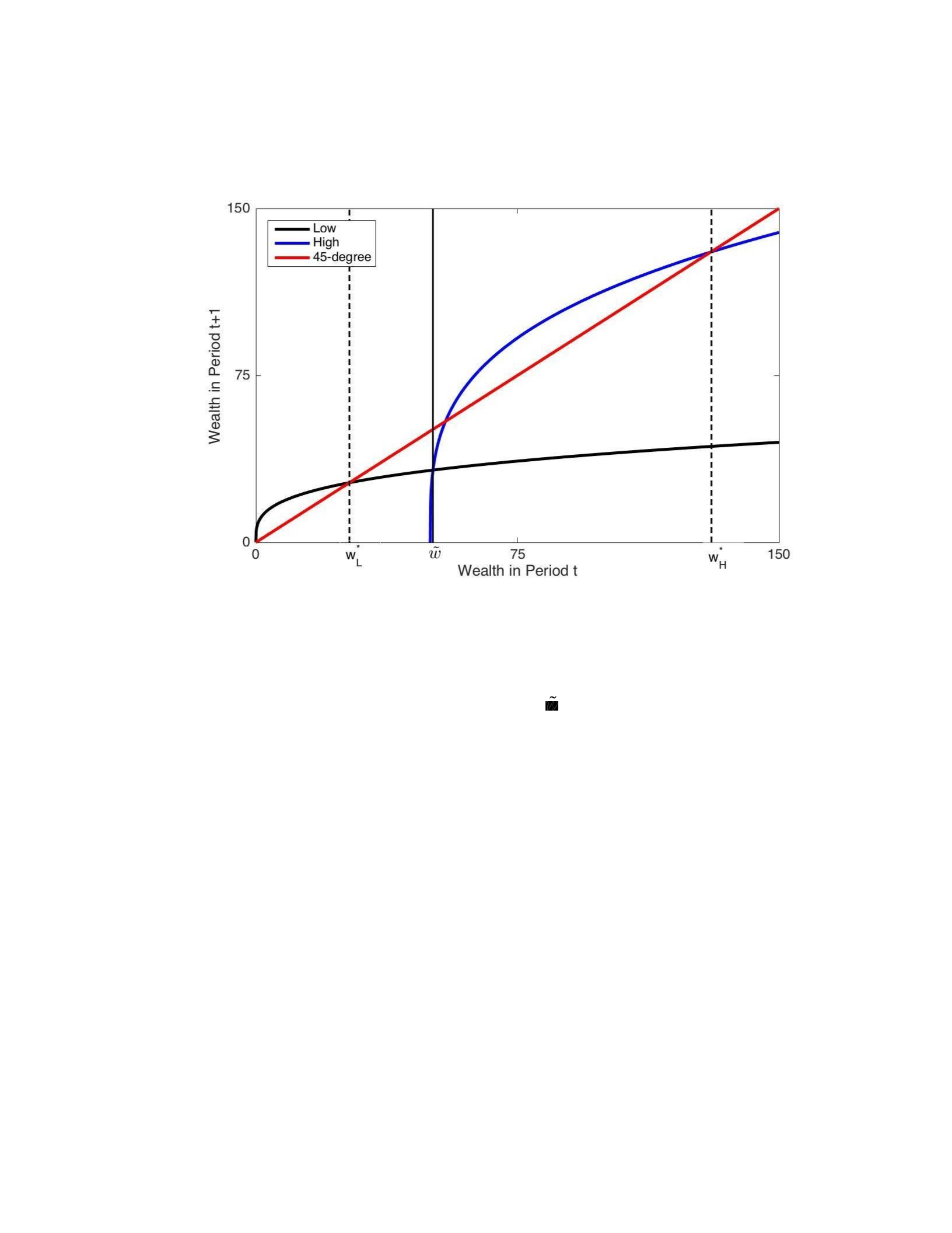
2.8 Tables and Figures

Figure 3.1: Individual Production Technologies

Notes: Figure shows the individual production technologies for low production

technology, in black, and the high production technology, in blue, capturing the change in

wealth from period t to period t+1. The red 45-degree line indicates where change in

wealth equals zero. The high and low equilibria are depicted where the respective

production technology intersects the 45-degree line, crossing from above. Additionally,

the figure depicts the technology switching point, , where the two production

technologies intersect.

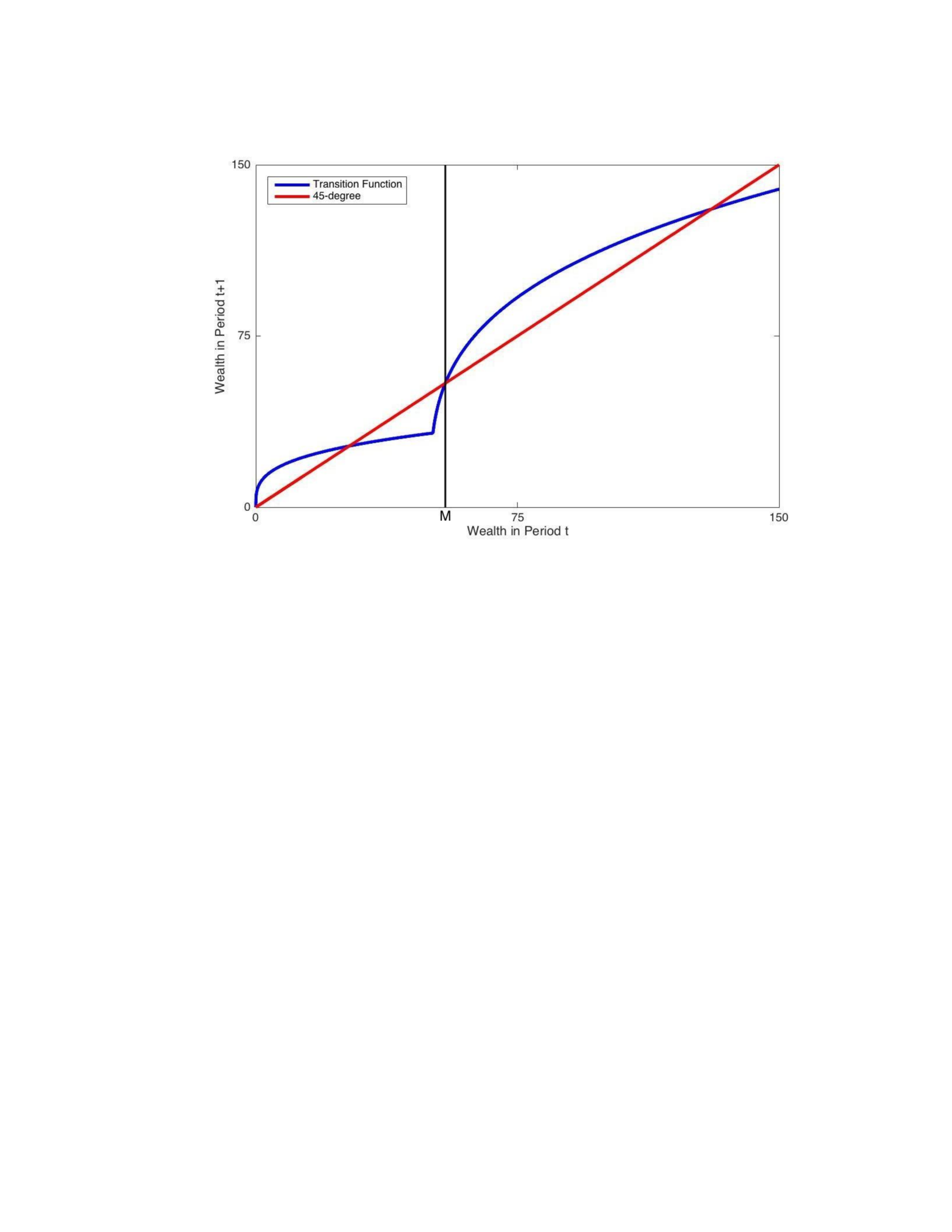
Figure 3.2: Transition Function

Notes: Figure shows the transition function, in blue, of wealth between periods before

stochasticity is introduced. The red line represents the 45-degree line. The Micawber

Threshold, M , occurs where the transition function crosses the 45-degree line from

below resulting in an unstable equilibrium.

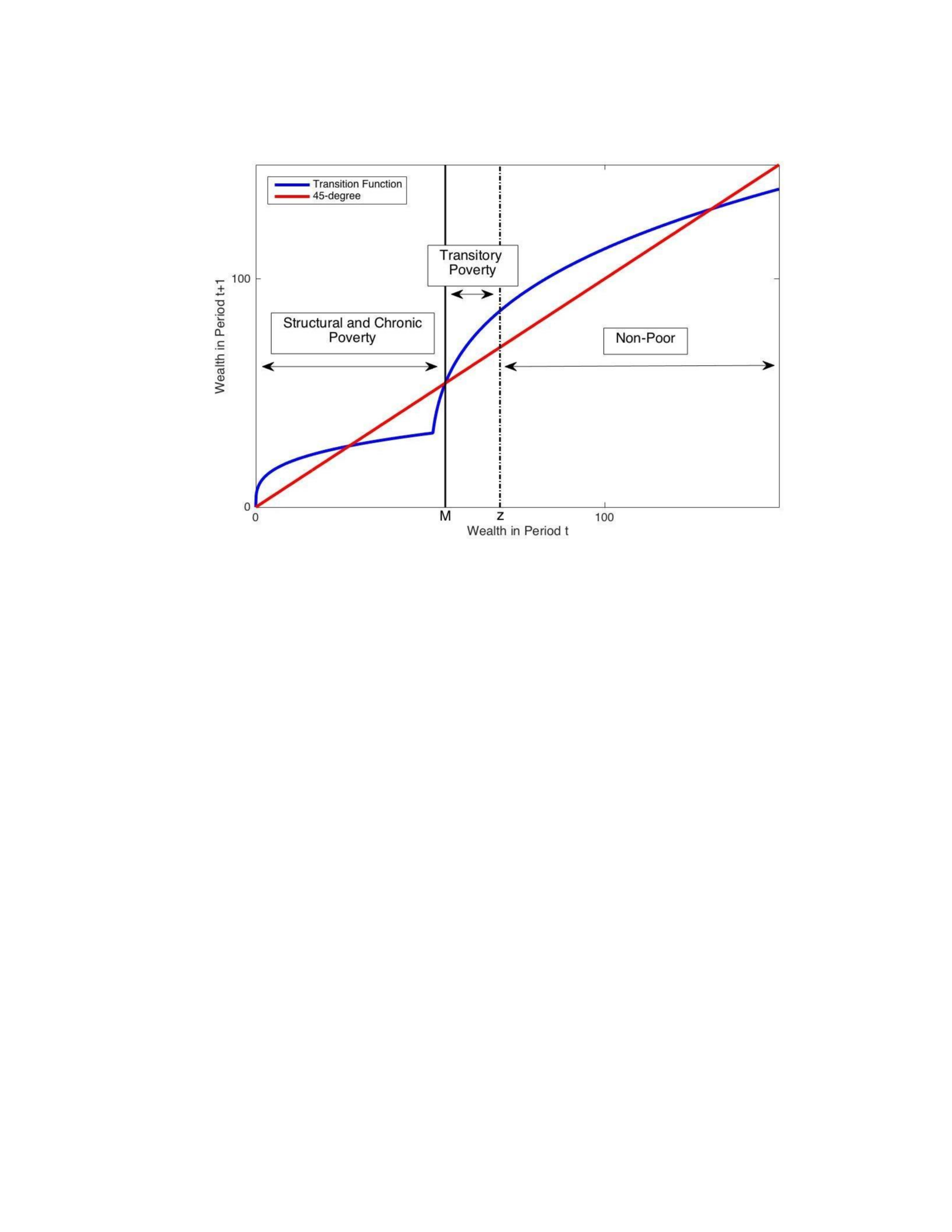
Figure 3.3: Transitory Poverty

Notes: Figure shows the transition function, in blue, of wealth between periods and the

45-degree line in red. The two vertical lines represent the Micawber Threshold, M and the

asset poverty line z, respectively, which are used to identify three regions: structural and

chronic poverty, transitory poverty, and non-poor.

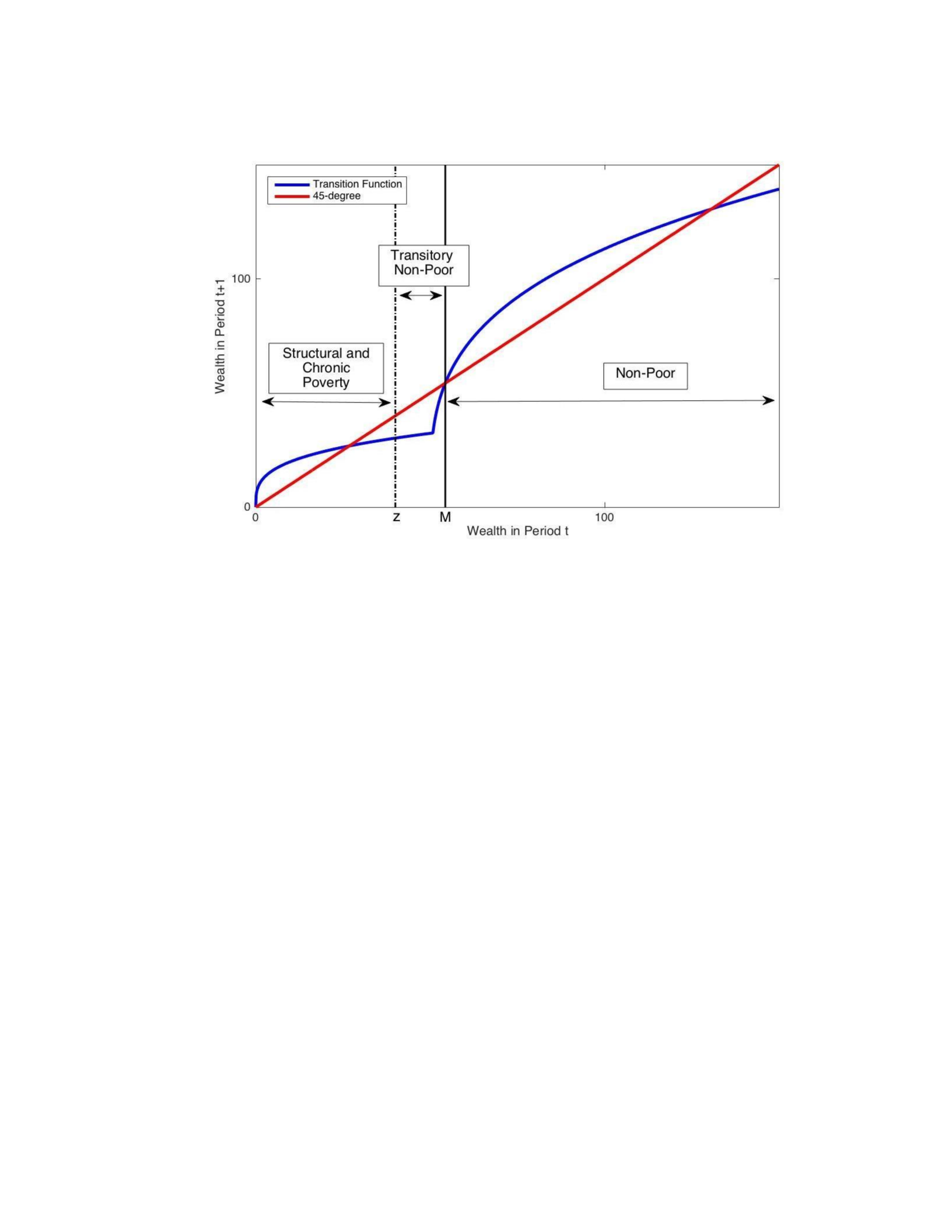
Figure 3.4: Transitorily Non-Poor

Notes: Figure shows the transition function, in blue, of wealth between periods and the

45-degree line in red. The two vertical lines represent the Micawber Threshold, M and the

asset poverty line z, respectively, which are used to identify three regions: structural and

chronic poverty, transitorily non-poor, and non-poor

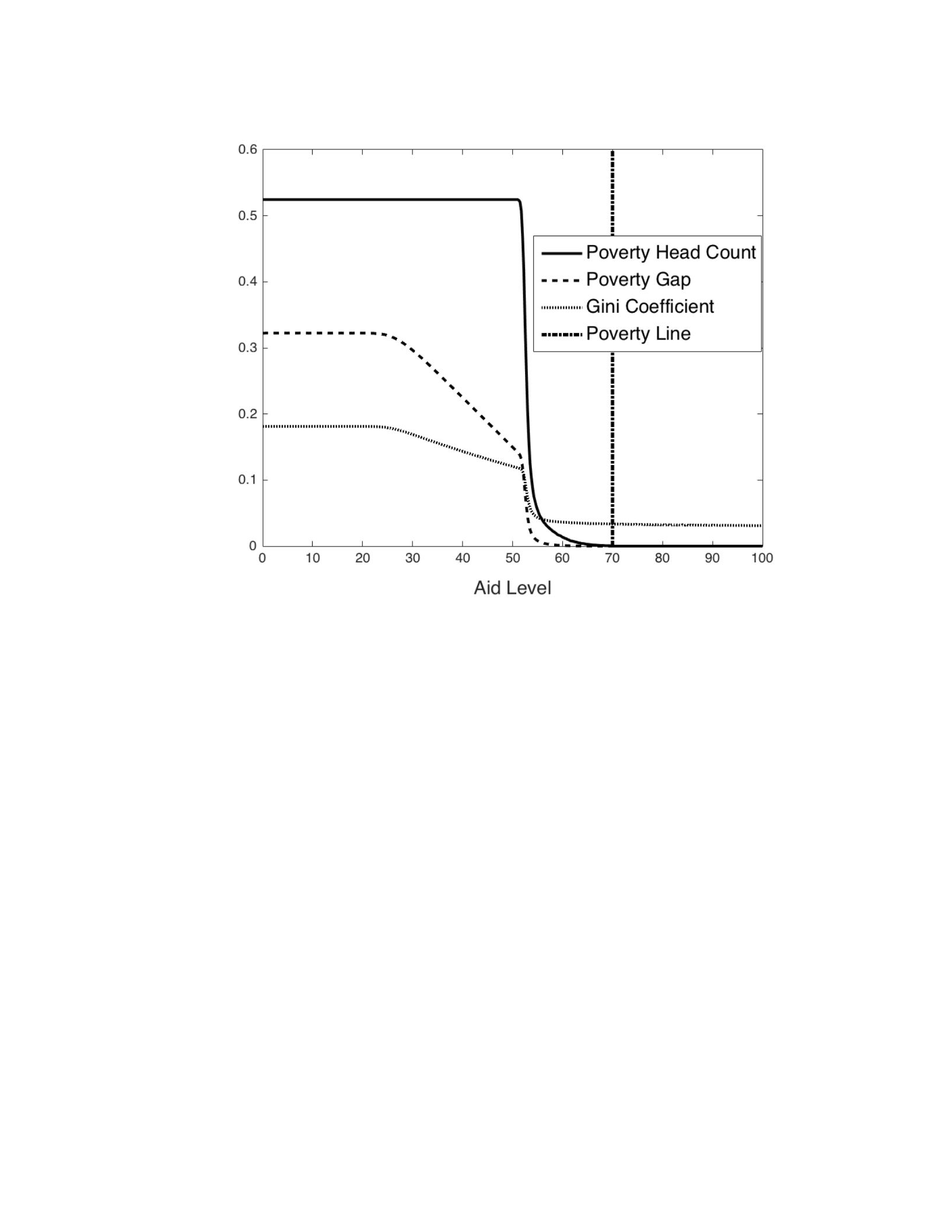
Figure 3.5: Poverty Measure Comparisons

Notes: Figure depicts the poverty measures: poverty headcount, poverty gap, and the Gini

coefficient expressed as function of aid level. These measures are calculated by

simulating wealth time paths with varying levels of aid and calculating each poverty

measure in every time period and taking the average of these values for the length of the

simulation. The Micawber Threshold for this parameter combination is at w 55, which

is just after the sharp drop in the poverty measures.

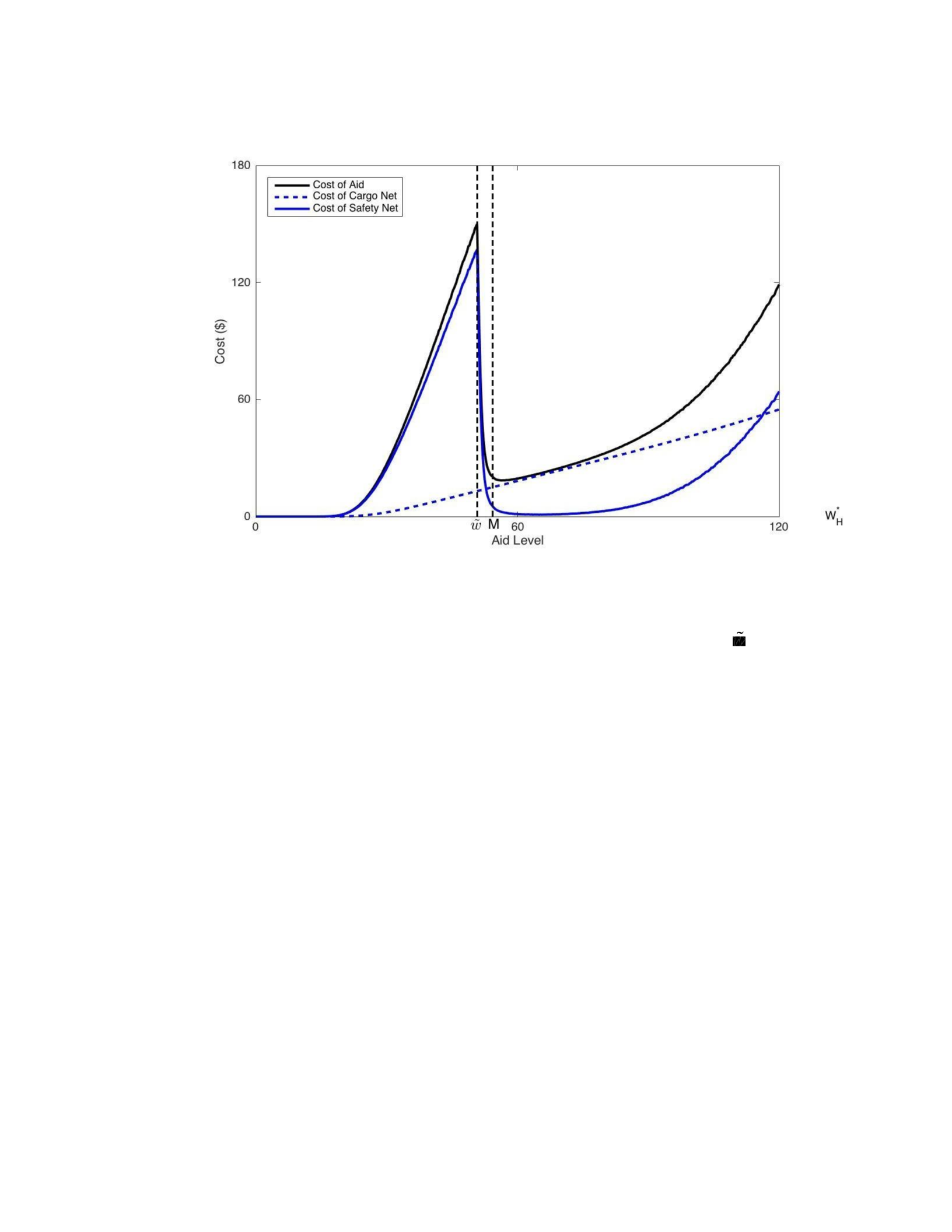
Figure 3.6: Poverty Measure Comparisons

Notes: Figure depicts the cost of providing aid in black as well as the separate cost of

providing a safety net, solid blue line, and the cost of providing a cargo net, dashed blue

line all as a function of level of aid. We see the cost of the safety net increases rapidly at

low aid levels then sharply dropping off at the technology switching point, and slightly

before the Micawber Threshold M. The cost of the cargo net is increasing with respect to

aid and does so at nearly constant rate (linear).

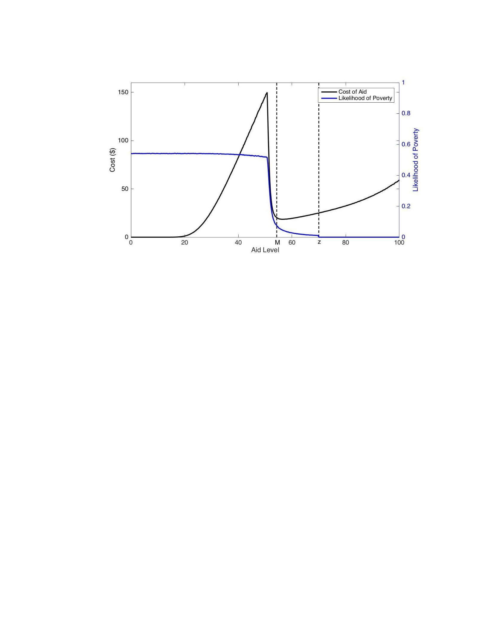
Figure 3.7: Cost of Aid and Likelihood of Poverty by Aid Level

Notes: Figure shows the cost of providing aid, in black, and the likelihood of poverty, in

blue, over a range of aid levels. The likelihood of poverty is the percentage of people

below the asset poverty line, z, throughout the simulation. The Micawber Threshold, M,

is also included.

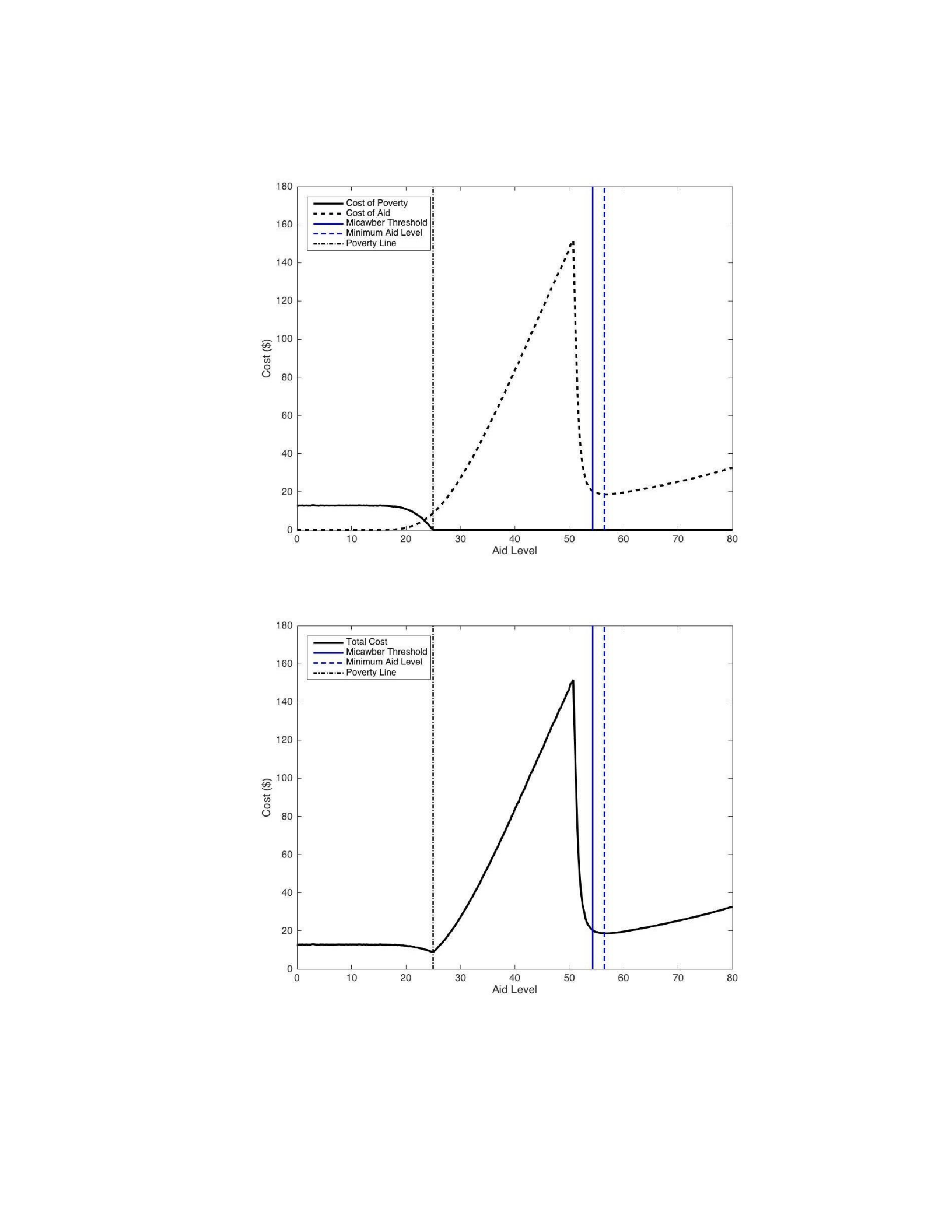
Figure 3.8: Costs with a low Poverty Line

Panel A: Individual Cost Curves of the Social Planner’s Problem

Panel B: Total Cost from the Social Planner’s Problem

Notes: Panel A depicts the cost of providing aid (solid black) and the social cost of

poverty (dashed black) while Panel B shows the total cost, which is the sum of the two.

The vertical lines in both panels are: poverty line (dashed black), the Micawber

Threshold (solid blue) and the minimum aid level (dashed blue).

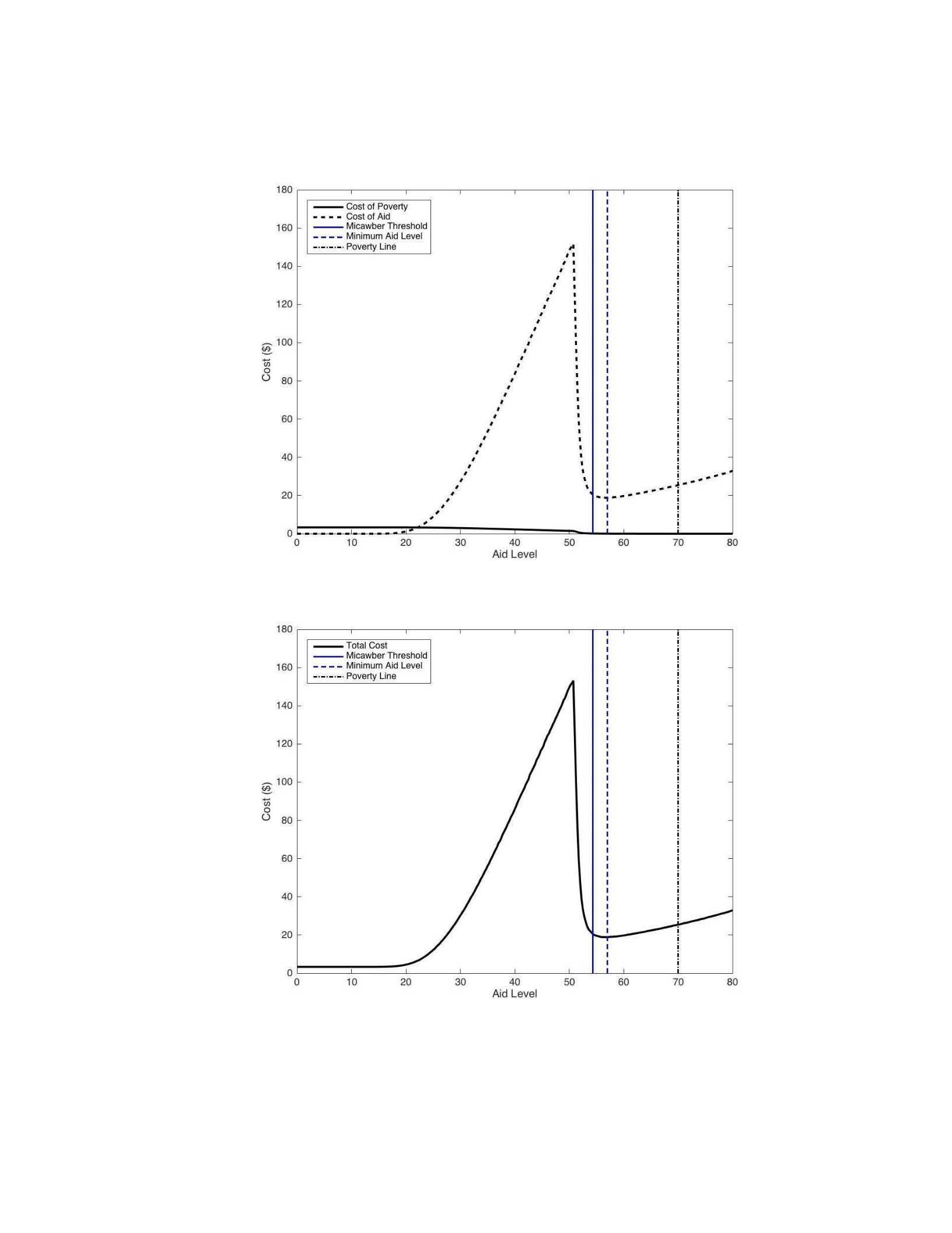
Figure 3.9: Costs with a Low





Panel A: Individual Cost Curves of the Social Planner’s Problem

Panel B: Total Cost from the Social Planner’s Problem

Notes: Panel A depicts the cost of providing aid (solid black) and the social cost of

poverty (dashed black) while Panel B shows the total cost, which is the sum of the two.

The vertical lines in both panels are: poverty line (dashed black), the Micawber

Threshold (solid blue) and the minimum aid level (dashed blue).

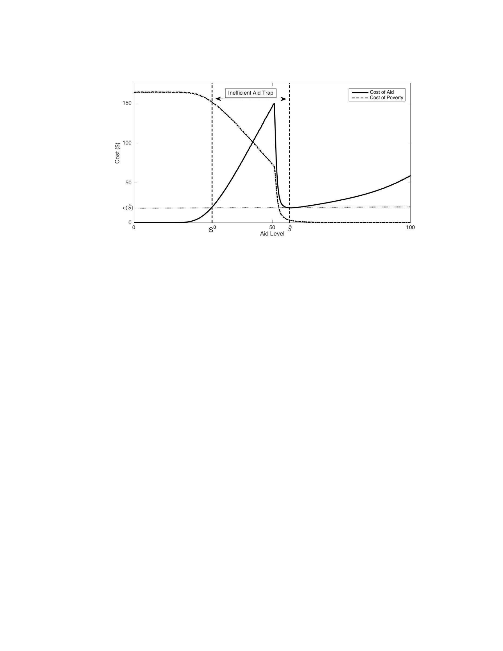
Figure 3.10: Inefficient Aid Trap

Notes: Figure shows the cost of providing aid, solid black line, and the social cost of

poverty, dashed black line, as well as the upper and lower bounds of the inefficient aid

trap,

and

0 respectively. The horizontal line occur

at c(S

ˆ), which

the c

ost

providing aid at Sˆ and S0. The region in between is inefficient because both cost of

providing aid and the social cost of poverty can be reduced.

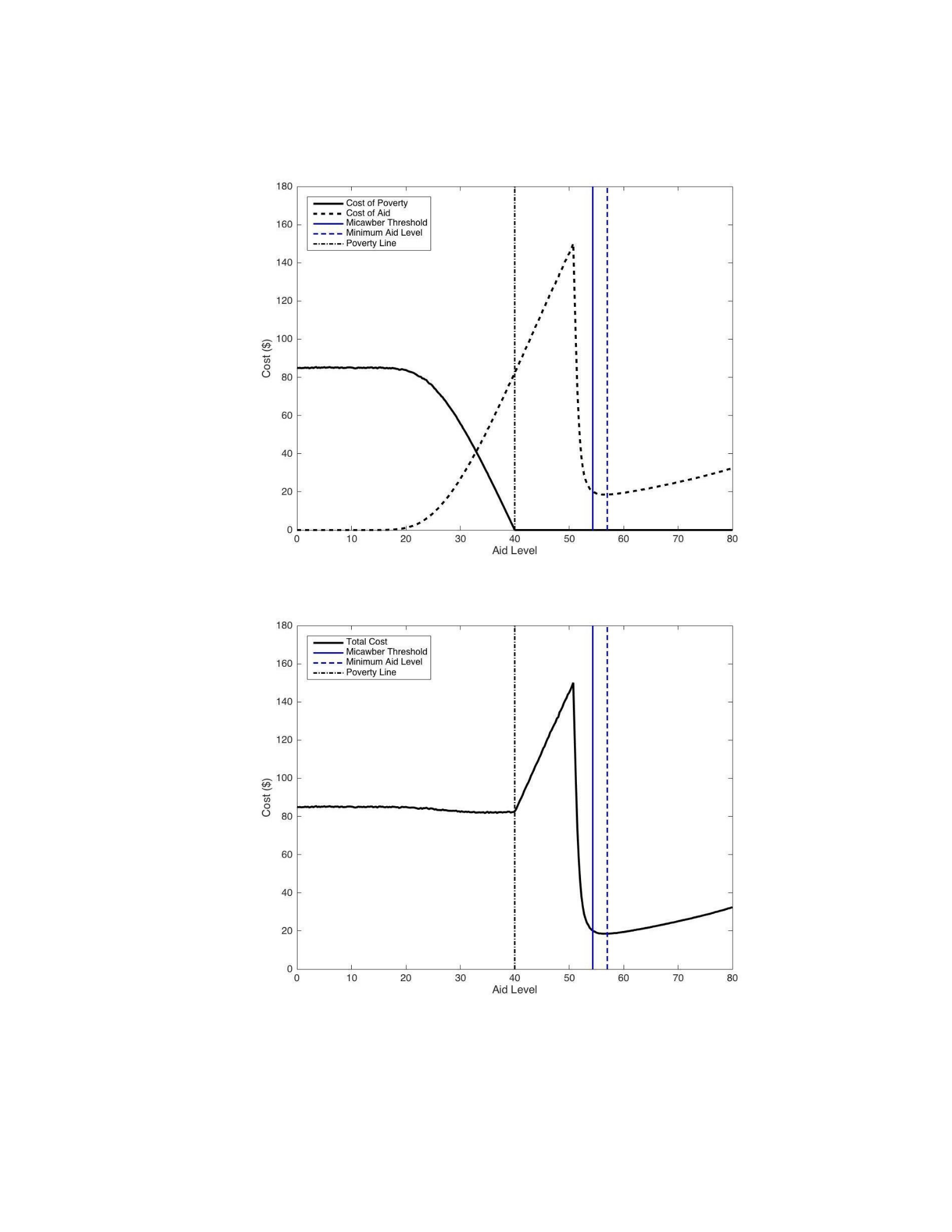
Figure 3.11: Costs with a Poverty Line Within Inefficient Aid Trap

Panel A: Individual Cost Curves of the Social Planner’s Problem

Panel B: Total Cost from the Social Planner’s Problem

Notes: Panel A depicts the cost of providing aid (solid black) and the social cost of

poverty (dashed black) while Panel B shows the total cost, which is the sum of the two.

The vertical lines in both panels are: poverty line (dashed black), the Micawber

Threshold (solid blue) and the minimum aid level (dashed blue).

Figure 3.12: Costs with a Poverty Line Above the Inefficient Aid Trap

Panel A: Individual Cost Curves of the Social Planner’s Problem

Panel B: Total Cost from the Social Planner’s Problem

Notes: Panel A depicts the cost of providing aid (solid black) and the social cost of

poverty (dashed black) while Panel B shows the total cost, which is the sum of the two.

The vertical lines in both panels are: poverty line (dashed black), the Micawber

Threshold (solid blue) and the minimum aid level (dashed blue).

Table 3.1 Effect of Micawber Threshold on Minimum Aid Level

(1)

(2)

(3)

VARIABLES

0.988***

0.992***

0.994***

(0.0027)

(0.0020)

0.0188***

0.0148***

(0.0004)

(0.0005)





0.888***

(0.0853)

Constant

1.778***

0.393***

0.352***

(0.1260)

(0.1000)

(0.0984)

Observations

3,108

R-squared

0.978

0.987

0.988

Adjusted R-squared

0.978

0.987

0.988

Notes: Regression show effect of Micawber Threshold on Minimum Aid level. Standard

errors are presented in parentheses and stars indicate significance level *** p<0.01, **

p<0.05, * p<0.1.

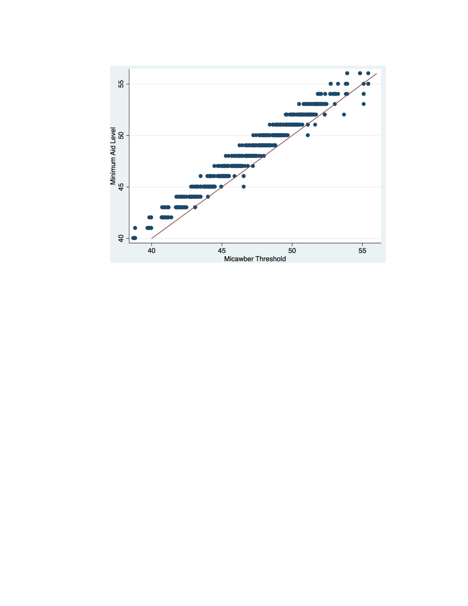
Figure 3.13: Relationship between Micawber Threshold and Minimum Aid Level

Notes: Figure shows the relationship between minimum aid level and the Micawber

Threshold. The red line is a 45-degree line; observations to the left/above the line indicate

the minimum aid level lies above the Micawber Threshold. Minimum aid level is an

integer as we vary aid level by integer values in the simulation.

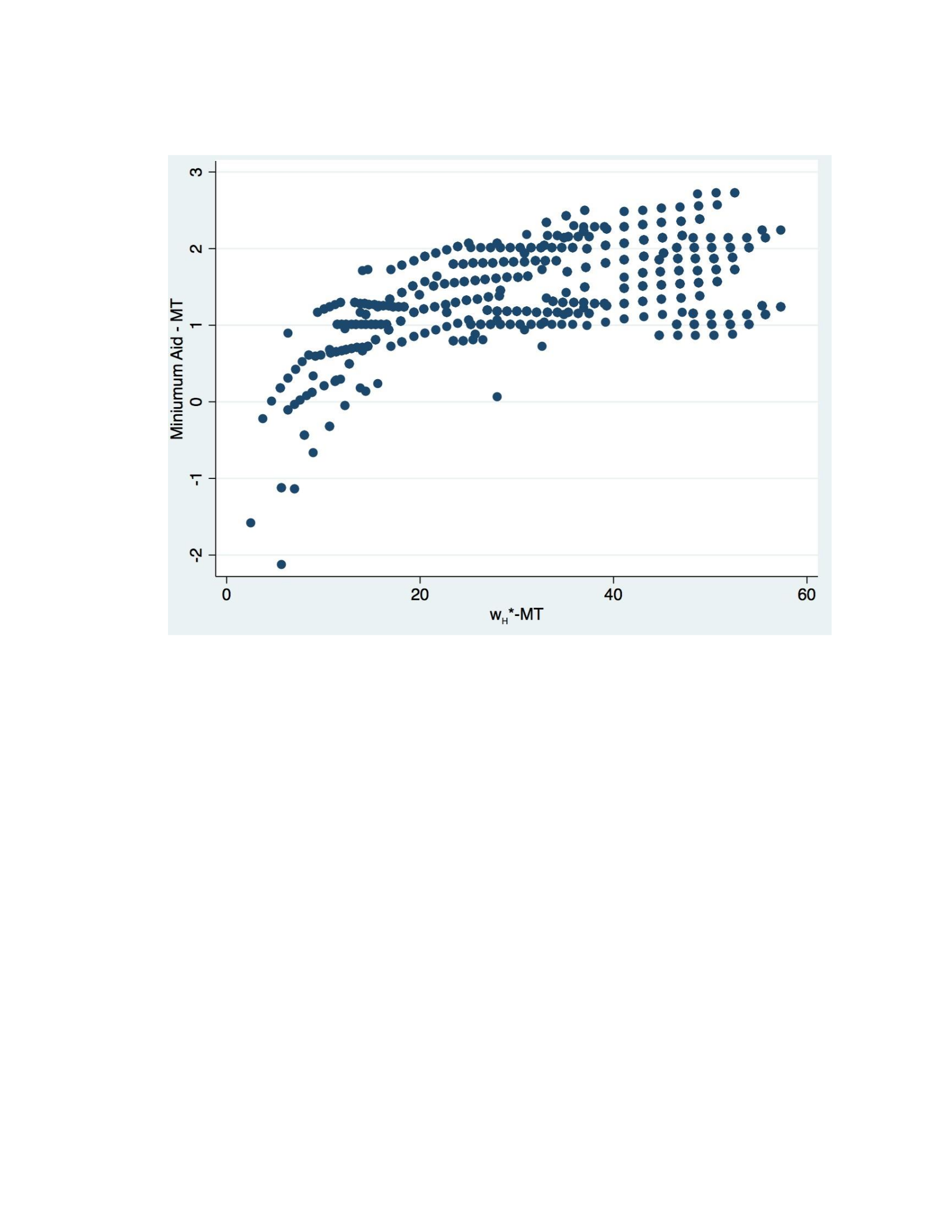
Figure 3.14: Effect of the difference between the high wealth equilibrium and MT

on the difference between minimum aid level and MT

Notes: Figure depicts the difference between the location of minimum cost of providing

basic wealth and the Micawber Threshold across different levels of the difference

between the high wealth equilibrium and the Micawber Threshold. Lower difference

between the high equilibrium and Micawber Threshold indicates a less stable high wealth

equilibrium, all else equal.

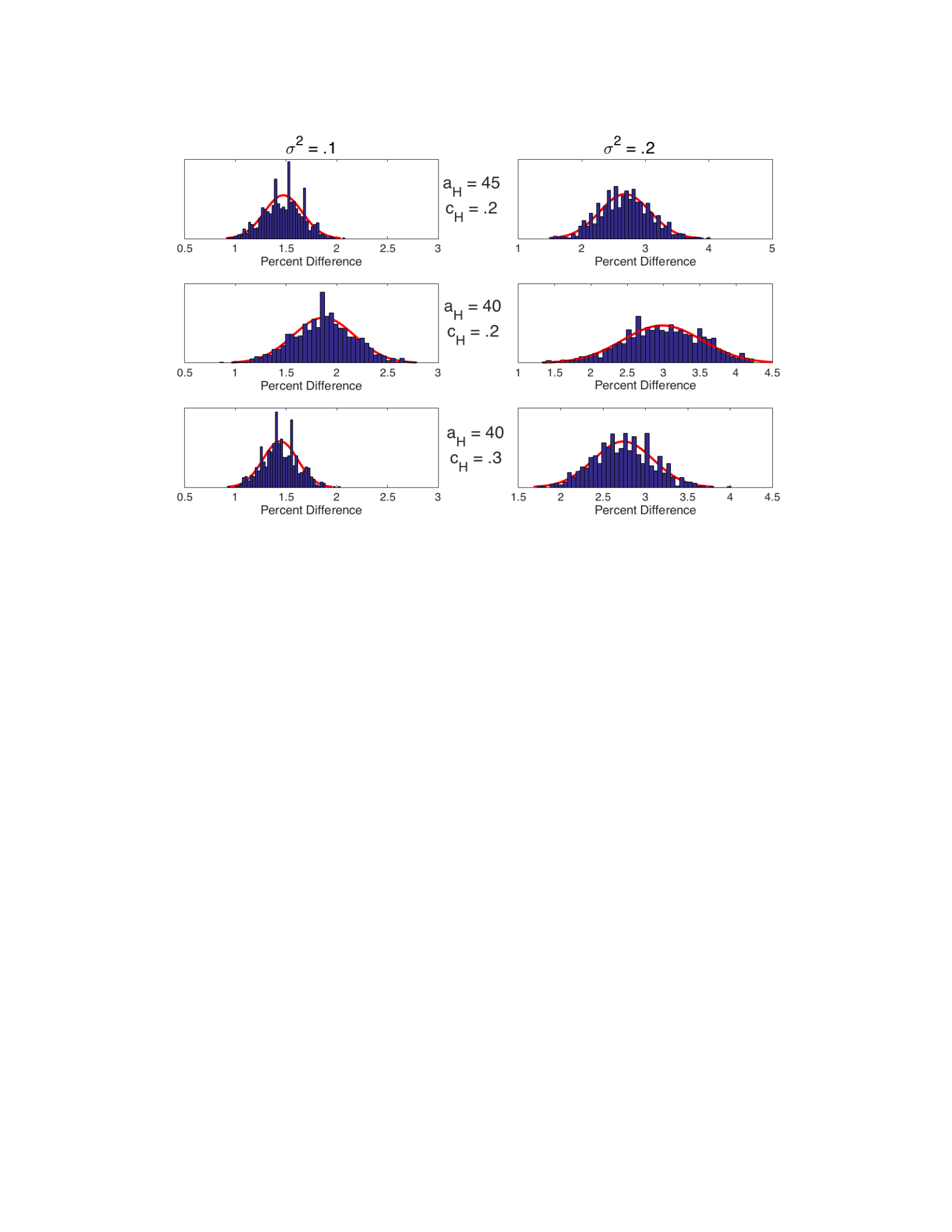
Figure 3.15: Percent Difference Between Minimum Cost of Aid and MT

Notes: Figure depicts the difference between the location of minimum cost of providing

basic wealth and the Micawber Threshold expressed as a percentage of the Micawber

Threshold. Each column has the same variance parameter and each row has the same

shape parameters. The histograms, in blue, show the density at each level of percent

difference and the red lines are the Gaussians fitted to the data. Data come from

simulating cost of providing basic wealth at various levels, with minimum cost defined as

the level of basic wealth resulting in a local minimum of cost. Simulation was performed

one thousand times for each set of parameters.

Table 3.2 Effects of Variables on Percent Difference

(1)

(2)

(3)

VARIABLES

Percent

Difference

Percent

Difference

Percent

Difference

-0.0810***

-0.0583***

-0.797***

(0.0056)

(0.0046)

(0.0379)

-0.160***

(0.0114)

0.919***

(0.0475)

-1.054***

(0.3120)





5.440***

5.453***

(0.138)

(0.134)

Constant

6.363***

4.288***

4.510***

-0.265

-0.223

-0.289

Observations

3,108

R-squared

0.063

0.375

0.453

Notes: Regression show effect of variables on the percent difference between the

Micawber Threshold and the Minimum Aid level. Standard errors are presented in

parentheses and stars indicate significance level *** p<0.01, ** p<0.05, * p<0.1.

4. Empirical Identification of a Multiple Equilibrium Poverty Trap

4.1 Introduction and background

There has been a long-standing difficulty in empirically identifying multiple equilibrium

poverty traps. This could be because existence of these wealth dynamics is relatively rare

or non-existent, the tools used to identify poverty traps are insufficient, or a combination

of the two. As discussed in section 3, multiple equilibrium poverty traps are distinct

phenomena under the umbrella of poverty traps. This chapter introduces two novel

methods of testing for multiple equilibrium poverty traps, by testing for necessary

features of asset transformation at the individual and village levels as well as in the

pooled data, which the data must exhibit if a multiple equilibrium poverty trap exists. We

perform these tests on the publicly available replication dataset where a poverty trap has

previously been found to exist, published under Lybbert et al. (2004). Unfortunately, we

find little evidence of a poverty trap in these data. Lybbert et al. find a multiple

equilibrium poverty trap consisting of two stable dynamic wealth equilibria, which we

refer to as a dual equilibrium poverty trap, by non-parametrically fitting a curve to the

data using kernel smoothing. Their identification of a dual equilibrium poverty trap is

simply a graphical observations of a non-convexity in wealth accumulation. However, we

find these data do not exhibit behavior necessary for a dual equilibria poverty trap,

namely mean reversion of wealth at the household level and two clusters of wealth

changes in the pooled data and for each village. The non-convexity in asset dynamics

found by Lybbert et al. (2004) may occur when fitting a curve to the data, but is not

indicative of a poverty trap. Instead the fitted curve may be picking up clustering in the

data more consistent with heterogeneous differences in asset levels and shocks over

villages in the sample. This chapter emphasizes the importance of using multiple tests to

ensure the data are consistent with an empirical model, in this case multiple equilibrium

poverty traps, rather than relying too heavily on curve fitting techniques which may cause

spurious overfitting.

There are many known issues surrounding the identification of poverty traps,

which Barrett and Carter (2013) discuss in detail, making them difficult to empirically

identify should they exist. First there will be very few observations around the Micawber

Threshold, the unstable dynamic equilibrium separating the basins of attraction between

high and low wealth equilibria. When the equilibria have substantial pull, few households

exist that switch between wealth equilibria. The nature of the unstable Micawber

Threshold rapidly pushes wealth away from it resulting in few observations around this

level. This makes it difficult to identify the location of the Micawber Threshold as well as

to observe the non-convexity in asset accumulation, which occurs at and below this point.

A second issue is it is difficult to distinguish between state dependence and

heterogeneous single equilibria. So even observing two clusters of wealth levels is not

sufficient to determine a multiple equilibrium poverty trap exists. In our analysis, we

circumvent these issues by answering the question of can a multiple equilibrium poverty

trap exist in our data, rather than does it exist. This distinction is important, as we do not

attempt to distinguish between these alternative hypotheses in this paper. Thus, we seek

to provide evidence against the existence of a multiple equilibrium poverty trap when it is

not present.

Another difficulty with identifying the multiple equilibrium poverty trap is

heterogeneous factors at the household level may allow for some households to

experience a multiple equilibrium poverty trap while others in the same population may

have only one dynamic equilibrium (e.g. Ikegami et al., 2016) or none at all (i.e. a

random walk). Given data constraints, most notably length of time and sampling

frequency, empirical estimation typically requires assuming a common underlying asset

dynamic for all households (Nashold, 2013, Jalan and Ravallion, 2004) exasperating this

issue. We surmount this issue by testing for mean reversion at the household level. This

test does not require an assumption of identical underlying asset dynamics.

There are also temporal issues that play a role. Micawber Thresholds may shift

over time due to changing market/environmental conditions making the identification of

unstable equilibria more difficult. This is problematic because identifying poverty traps

usually requires a dataset spanning large time intervals increasing the likelihood of a

changing Micawber Threshold. Using cross-sectional data does not provide enough

information to identify a multiple equilibrium poverty trap, as it does not capture the

wealth dynamics. A multiple peaked cross section of wealth levels is neither necessary

nor sufficient to indicate a poverty trap. Thus, we need to look at assets over time. A long

sampling period is desirable because many of the tests for multiple equilibrium poverty

traps rely on asset based measures, which are slow to change over short samples. The

methods we present do not help alleviate these issues and require assuming any dynamic

equilibria are stable over time.

These issues have been used to explain why poverty traps have been so difficult to

identify in practice even in socio-economic environments where theory suggests they are

likely (e.g. Jalan and Ravallion, 2004; Lokshin and Ravallion, 2004; Kraay and Raddatz,

2006;Nashold 2013; McKay and Pergee, 2014). These papers all seek to identify poverty

traps in rural areas of Southern Africa with limited access to financial markets, and few

potential livelihoods (mostly subsistence farming and pastoralism). Barrett and Carter

(2013) make the case that failing to find multiple equilibrium poverty traps should not be

interpreted as evidence against the existence of poverty traps. The authors take the stance

that many of the empirical difficulties involved likely cause researchers to fail to identify

poverty traps in cases where they exist. A major contribution of this chapter is we design

falsification test designed to look for necessary conditions of the poverty trap without

attempting to identify the Micawber Threshold explicitly, as there are many difficulties in

attempting to locate it, which we discuss below.

The empirical literature has seen numerous strategies attempting to directly

identify the elusive multiple equilibrium poverty trap by estimating wealth dynamics,

especially attempting to identify non-convexities in wealth growth over certain ranges as

well as locating stable and unstable dynamic equilibria. The direct measures can be

broken down into three categories based on identification methods. Nashold (2013),

provides an in depth discussion of these. The first methods were fully parametric methods

that fit some polynomial function, which allow for some non-convexities (i.e. cubic and

higher order) and identify whether the estimated function results in multiple dynamic

equilibria (e.g. Jalan and Ravallion, 2004; Santos and Barrett, 2011). These models are

overly restrictive, as they require specifying a cubic or quadratic function to the data.

Alternatively, non-parametric techniques allow for more flexibility by not

restricting estimation to fit a specific functional form and have been successful in

identifying poverty traps in some contexts (e.g. Adeto et al., 2006; Barrett et al., 2006);

this is the technique used by Lybbert et al. (2004). These techniques fit kernel, or other

smoothing functions, to the data to look for non-convexities in wealth accumulation,

providing more flexibility than the parametric techniques. While more flexible, the non-

parametric fitting still requires substantial observations around the non-convexity and the

Micawber Threshold, which are rarely occurring. In fact, having enough data to fit the

non-convexity with any degree of confidence either requires a massive data set or is

indicative of a lack of a poverty trap.

The Micawber Threshold necessarily represents an unstable dynamic equilibrium,

which, in essence, is constantly pushing wealth away from it. This must result in the

distribution of wealth levels will be more disperse around this point making the

likelihood of observing wealth in this area should be low. Failing to account for this is

problematic and may lead to spurious identification of multiple equilibrium poverty traps

when they do not exist. Previous identification strategies have treated the identification of

a non-convexity as sufficient evidence of a multiple equilibrium poverty trap, however it

is merely a necessary condition of one. A non-convexity found by fitting a curve through

a large cluster of data is inconsistent with a multiple equilibrium poverty trap making this

form of identification insufficient to determine a multiple equilibrium poverty trap to

exist. The curve fitting approaches, both fully parametric and semi-parametric, have

typically not accounted for the likelihood of observations and are prone to over

identifying poverty traps in this maner, which we show is likely the case for the findings

in Lybbert et al. (2004) using their replication data.

Nashold (2013) analyzes the effectiveness of the fully parametric and non-

parametric methods of directly observing poverty traps and recommends using semi-

parametric techniques to combine the flexibility of non-parametric techniques with the

ability to control for household characteristics and time fixed effects (Nashold, 2013).

Using household data from Pakistan and Ethiopia, Nashold (2013) assess the

effectiveness of numerous means of testing for poverty traps and finds one unique

dynamic equilibrium around the same level using a parametric, non-parametric and semi-

parametric methods. While Nashold holds the semi-parametric approach will perform

better when there are non-convexities underlying the multiple equilibrium poverty traps,

the semi-parametric methods still face many of the challenges of the direct measures

most notably a lack of observations around the non-convexity.

More recently, Barrett and Carter 2013, among others, have begun using indirect

methods of testing for poverty traps, which circumvent many issues of the direct

approaches. These indirect methods seek to identify behaviors, which are consistent with

multiple equilibrium poverty traps. These methods seek to identify behaviors, which

would only be rational if individuals were indeed facing a multiple equilibrium poverty

trap, such as asset smoothing at certain wealth levels (Zimmerman and Carter, 2003;

Carter and Lybbert, 2012), exhibiting risk seeking behavior when assets are just below a

Micawber Threshold (Lybbert and Barrett 2011), or avoiding providing gifts and loans to

households near the Micawber Threshold (Santos and Barrett, 2011). These techniques

bypass many of the empirical challenges presented in Barrett and Carter (2013) and show

signs of being able to improve our ability to identify MEPT.

These indirect methods do not rely on identifying the non-convexity in wealth

accumulation nor require locating the Micawber Threshold. A benefit of indirect

estimation is it typically does not require assuming an underlying wealth dynamic for all

households, as is typically required for the direct measures, as many of the implications

of poverty traps can be specified in a way to require a smaller sample size and can be

done at the individual level. Testing for non-convexities at the individual level is near

impossible, while testing for specific savings and consumption decisions should be done

at the individual level. Thus these methods should perform better than direct methods

when heterogeneity across individuals may result in different wealth equilibria within a

sample by being able to distinguish between these competing hypotheses.

In this chapter, we introduce two novel indirect tests, which can be used to rule

out the existence of a multiple equilibrium poverty trap. Rather than identify the

Micawber Threshold or the non-convexity in wealth dynamics, in-line with previous

direct test, we focus on identifying trends in the data that are consistent with the existence

of dynamic equilibria. We test for dynamic equilibria in two ways: (1) testing for mean

reversion using a variance ratio test at the individual level, and (2) using a mixture model

to determine if there is clustering in the pooled data and for each village, which would

indicate multiple dynamic equilibria.

If a dynamic wealth equilibrium exists, then we should observe wealth trending

towards it over time with some random error, in other words we should observe mean

reversion. When there exist multiple dynamic equilibria, we should observer mean

reversion so long as wealth remains in the basin of attraction of one equilibrium.

However, once the Micawber Threshold is crossed due to the stochastic nature of wealth

dynamics, wealth will tend towards a different equilibrium making it more difficult to

identify mean reversion in the sample. The nature of multiple equilibrium poverty traps

makes it relatively rare for these thresholds to be crossed, resulting in the few

observations around Micawber Thresholds (Barrett and Carter, 2013) ensuring the

majority of the sample will not have this issue.

We test for mean reversion of wealth at the household level using a variance ratio

test. While the existence of mean reversion for an individual is a necessary condition for

the existence of a multiple equilibrium poverty trap, it is also occurs in the case of one

dynamic wealth equilibrium. This mean reversion is a necessary, but not sufficient

condition of a multiple equilibrium poverty trap. The variance ratio test is used to test the

hypothesis that the rate of return of an asset (in our case the change in wealth from one

period to the next) is independent over time, indicating a random walk. It rests on the

known statistical property that the summation of two independent random variables will

have a variance equal to the sum of the two. Thus, an independent time series will exhibit

additive variance of the rate of return (change in wealth) as the time-step increases, which

is used to construct the null hypothesis of a random walk. The variance ratio test has been

widely used in the finance literature to determine whether financial asset prices are mean

reverting, trend following or if they follow a purely random walk (e.g. Lo and

MacKinlay, 1988). We test this at the household level and do not find statistically

significant evidence of mean reversion in our data. In principle, this test can be done with

the pooled and at thevillage level, but is unlikely to identify mean reversion unless

household equilibria are clustered together. We find slightly over 5% of individuals

exhibit mean reversion, which is not significantly different than what we would expect to

find due to random chance. This is evidence against the existence of dynamic equilibria

for individuals and, therefore, evidence against the existence of the dual equilibria

poverty trap found by Lybbert et al. (2004). While this test rules out a multiple

equilibrium poverty trap, we also fit a mixture model to the data at the village level and

with the pooled data and find further evidence against the existence of multiple

equilibrium poverty traps. We find some evidence concerning potential spurious

overfitting by Lybbert et al. (2004) by identifying a cluster of data near the Micawber

Threshold identified in their paper.

Finite mixture models have been used to empirically classify individuals into

different groups or ‘clusters’. A finite mixture model is essentially a form of latent class

modeling intended to identify different classes of individuals within a population

(Harrison and Rutström, 2009). It can be used to both identify the number of clusters

within a dataset as well as predict assignment of individuals to each cluster. In

economics, finite mixture models have been predominantly used to determine behavioral

decision rules when playing games or making complex decisions (Bruhin et al., 2010;

Conte et al., 2010; Sproul and Michaud, 2017). In the development field, finite mixture

models have been used to look at informal employment (Günther and Launov, 2009) and

even wealth dynamics at the macro-level (Alfo et al., 2008; Owen et al., 2009). Alfo et al.

(2008) find the Solow growth model performs better when allowing for multiple

heterogeneous groups fitted from a finite mixture model. Similarly, Owen et al. (2009)

find multiple single equilibria at the macro-scale, which is best predicted by institutional

features rather than factors such as region or income. We perform a similar analysis at the

micro-scale, while focusing on using the fitting of the mixture model to test for multiple

equilibrium poverty traps.

We fit a mixture model to the pooled data and for each village in an attempt to

observe clustering consistent with the dual equilibria poverty trap found in Lybbert et al

(2004). The larger scales have the benefit of larger sample size, but at the cost of any

heterogeneity within the sample potentially obscuring the multiple equilibrium poverty

trap, should it exist. However, a mixture model fit at the individual level runs the risk of

over fitting due to small sample size. It also should fail to observe clustering around

multiple equilibria for those stuck at a single equilibrium and will prefer a single

component mixture. We find no evidence to support the existence of the dual equilibria

poverty trap using the mixture model. Depending on the criteria used to select the best fit,

which we discuss in the methods section, we find either the one cluster or three cluster

model is fits the data better for the pooled data as well as at the village level. We perform

a numeric simulation to show AICc and BIC perform well at fitting the two cluster model

when it exists, indicating we either have more than two equilibria or wealth dynamics

follow a random walk, both of which are inconsistent with the Lybbert et al. (2004)

findings.

While neither test is sufficient to determine the existence of a multiple

equilibrium poverty trap, both test for necessary features. Using the data from Lybbert et

al. (2004) we find the data does not exhibit mean reversion at the individual level and do

not find evidence of clustering consistent with the dual equilibria poverty trap found by

Lybbert et al. (2004) using pooled data or at the village level. These tests can be used to

rule out the existence of a multiple equilibrium poverty trap, but do not help us in

distinguishing between alternative hypotheses such as heterogeneous dynamic equilibria

for individuals, which we save for future work. These methods circumvent the issues

surrounding the direct tests for multiple equilibria, as they do not require identifying

neither non-convexities nor the location of a Micawber Threshold. Thus, these tests are

most useful as a first pass at identifying a multiple equilibrium poverty trap or as a

falsification test for previous empirical studies where poverty traps have been reported.

4.2 Context and data

Our data come from pastoralists in the Borana Plateau of Southern Ethiopia over 17 years

from 1980-1997, which Lybbert et al. (2004) have used previously to identify a dual

equilibrium poverty trap. The data contain 55 randomly selected households from four

villages10. From these 55 households, we restrict our sample to households with at least

10 years of data leaving us with 49 households from four villages. The data contain

information of household size, herd size, animal births, animal mortality, herd sales, herd

gifts, and a measure of rainfall. Lybbert et al. (2004) show sales represent an insignificant

portion of herd loss and gifting/loaning animals is relatively limited so we do not separate

these factors from herd mortality. For our analysis we focus on herd size per capita, in

line with previous poverty trap literature for the region (e.g. Lybbert et al., 2004, Barrett,

2005; Toth, 2014).

An important caveat to the data is it only includes information for pastoralists

active in 1997 (Lybbert et al. 2004). Any households that exited the sample during the

study period are not included. Through discussion with pastoralists in the area, Lybbert et

el (2004) state those exiting pastoralism were households with small herds coupled with

negative shocks from drought, disease or distress sale with no households ‘graduating’

10 Village membership refers to a household living near the geographic village center

over the course of the sample. Village membership is stable with the typical household

being part of the same village for multiple generations.

out of pastoralism due to high wealth levels. Thus, there is an upward attenuation bias

present in the sample. Failing to observe the households forced out of pastoralism

potentially obscures a low-level Micawber threshold below which pastoralism altogether

becomes unsustainable. However, we should still be able to identify a multiple

equilibrium poverty trap arising from the switching between sedentary pastoralism and

mobile pastoralism even with the attenuation bias.

The data we use may not be identical to the final data used in Lybbert et al.

(2004). When we received the data from Travis Lybbert, he explained the code for their

analysis as well as their finalized version of the data were lost due to a computer failure.

We have had substantial difficulty in recreating some of their results using this data set,

which is also publically available alongside their publication. The inability to replicate

results is problematic for conducting a conclusive falsification test of the Lybbert et al.

(2004) results, but we proceed with our analysis to test for a multiple equilibrium poverty

trap within the data we were able to obtain.

The Borana Plateau is characterized as arid and semi arid lands (ASAL). As

discussed in sections 1 and 3, the pastoralist system of the ASAL is an ideal context to

study poverty traps. There are apparently similar groups, mobile pastoralists and

sedentary households, with very different outcomes. A compelling explanation is there is

a critical herd size, which is their primary form of wealth and productive assets, above

which households can engage in the more lucrative mobile pastoralism, but below which

requires the household to stay near the village resulting in a dwindling herd and possible

exit from pastoralism altogether. This phenomenon arises due to less grazing area

accessible to sedentary pastoralists, which is potentially exacerbated by the ‘tragedy of

the commons’ in which sedentary herds over graze the pastureland close to the village.

4.3 Wealth Dynamics

How wealth changes over time is the fundamental question of the poverty trap literature.

The multiple equilibrium poverty trap describes the case where similar households have

access to multiple long-term stable equilibria depending on initial asset levels, where at

least one of these equilibria lies below some poverty line. See chapter 3 for a more

detailed discussion of the theoretical mechanisms, which result in multiple equilibrium

poverty traps. We seek to distinguish this from alternative hypotheses of heterogeneous

single equilibria and that assets follow a random walk.

The random walk hypothesis is typically seen in the financial literature to model

stock prices. This occurs when changes in assets are independent over time. If this occurs

and we plotted changes in wealth in wt and wt 1 space, we would see observations

spread across the 45-degree line, which is interpreted as where wt wt1 opposed to

clustering around points on the 45-degree line. Household wealth would fluctuate in a

random manner around the 45-degree line. Large deviations from the 45-degree line are

possible due to large random shocks such as drought. If we took a cross section of wealth

at any time period, we would expect to observe something similar to a normal

distribution of wealth with a high variance, as the variance of the distribution should be

increasing over time. At the individual level, we would not observe clustering of wealth

levels and would not observe mean reversion, as the fluctuations are independent over

time. We use the random walk model to construct the null hypothesis to test for mean

reversion using the variance ratio test, which we describe in the methods section.

Alternatively, each household could have unique dynamic wealth equilibria,

which the household would tend toward over time, absent stochastic fluctuations. For the

pooled data, if households in a sample share a similar equilibrium we would observer a

single cluster of wealth around one point on the 45-degree line, rather than observations

being more dispersed across it as in the random walk case. However, if there is

substantial heterogeneity in the location of household equilibria, changes in wealth may

appear identical to the random walk case in the pooled data and we would observe

changes in wealth dispersed across the 45-degree line without much evidence of

clustering around any points. However, at the individual level, we would observe

significant mean reversion and clustering of wealth levels around a single equilibrium for

each individual.

The last case we consider is when multiple dynamic equilibria exist for

households. If these equilibria are similar across households in the sample, we would

observe clustering around each equilibrium. The further spaced the equilibria and the

stronger the pull each equilibrium has will determine exactly how separate these clusters

will appear. Once again, if there is substantial heterogeneity, we may observe wealth

changes dispersed across the 45-degree line rather than appearing as clusters. At the

individual level, we would see the majority of households with a single cluster of wealth

levels identical to the case of a single equilibrium, as most households will remain in the

basin of attraction of a single equilibrium. However, we will observe some instances of

clustering followed by a sharp change (large deviation from the 45-degree line) followed

by clustering at a new level. This would indicate a Micawber Threshold was crossed and

wealth levels are tending towards a new equilibrium for the remainder of the sample.

The dynamics highlight the importance of looking at the individual level to

identify multiple equilibrium poverty traps when there is large heterogeneity amongst a

population, which is potentially unobservable. However, this dramatically reduces the

sample size reducing the power of statistical tests; in our data, for example, T 17.

Many of the direct measures for identifying poverty traps may not be appropriate at such

a fine scale, which is why most of the poverty trap literature has looked at the pooled data

or village level and assumed an underlying asset dynamic across the sample (Jalan and

Ravallion, 2004; Nashold, 2013). However, the two techniques we present do not require

as large a sample size as we do not attempt to identify the Micawber Threshold nor a

non-convexity in wealth dynamics, both of which require observing relatively rare wealth

levels around the unstable Micawber Threshold.

Figure 4.1 presents a summary of how assets evolve over time in our dataset. The

left panel shows a histogram of changes in log wealth. We see large left-tail indicating

large downward shocks, consistent with large drought or disease. The second graph

depicts the absolute distance from the mean of the sample. We would expect this to

follow the right half of a normal distribution, as we cannot have negative values, for

either a random walk or a single equilibria. The flatter the distribution, the more

consistent data are with a random walk as observations will be more evenly dispersed

across the 45-degree line rather than grouped around an equilibrium. If we observer

multiple peaks, it is indicative of a multiple equilibria, either due to a multiple

equilibrium poverty trap or clustering of heterogeneous single equilibria. The third panel

shows the relative distance from the mean where the negative values indicate x-values

below the mean x-value. Once again, observing multiple peaks would be consistent with

multiple equilibria, which we do not observe in the pooled data. We see similar results

for each village as well.

4.4 Methods

We present two new indirect falsification tests for the existence of a multiple equilibrium

poverty trap. Rather than attempting to identify poverty traps, in line with much of the

previous literature, we identify necessary conditions for the multiple equilibrium poverty

trap at three scales: in the pooled data, at the village level, and at the household level to

determine if the multiple equilibrium poverty trap may exist. In the pooled data, it seems

unlikely to find evidence of a poverty trap, as it would require households across

different villages with varying socio-economic conditions to have similar dynamic

equilibria. For example, Table 4.1 shows the average wealth by village. We see

substantial differences in mean wealth and standard deviation, which indicates different

socio-economic conditions between villages. If there exists substantial heterogeneity in

dynamic equilibria, should they exist, for households and/or villages, it will be difficult to

find evidence of the multiple equilibrium poverty trap even if it exists. However, Lybbert

et al. (2004) do identify a poverty trap using the pooled data, using a similar dataset, by

directly identifying a non-convexity in wealth accumulation even with these issues. At

the village level it will be more likely to be able to identify a multiple equilibrium

poverty trap when it exists. Within a village, many of the socio economic conditions

faced by individuals will be similar. Thus, the underlying cause of the poverty trap may

be shared by households resulting in similar dynamic wealth equilibria. However,

heterogeneity in ability between households may still play a major role in the existence

and location of Micawber Thresholds separating dynamic wealth equilibria. Ikegami et

al. (2016) use a theoretialc model to show how heterogeneous individual ability can result

in some households experiencing a multiple equilibrium poverty trap while low-skilled

individuals may only have access to a low equilibrium and high-skilled individuals a high

wealth equilibrium. This is justification to attempt to identify multiple poverty traps at the

individual level as well.

Lybbert et al., (2004) report herd accumulation to be highly correlated with herd

size. Using transition matrices based on quartiles of herd size, they find a household in

the lowest quartile of herd size has a 92% chance of remaining in the lowest quartile in

10 years. On the other side, less the 3% of households in the upper quartile drop into the

lower quartiles in the next year and only 9% after 10 years. This indicates a relatively

stable wealth relationship between households and low occurrence of transitory poverty.

The poor households stay poor while the wealthier ones stay on top. While consistent

with the poverty trap hypothesis, these wealth dynamics are also consistent with other

explanations. It could indicate distinct groups of households, where the more able

households tend to stay wealthier over time. Or it could simply be each household has its

own random walk with low enough variability that moving between quartiles is relatively

rare. While we do not attempt to distinguish between multiple groups and the MEPT, we

can test for whether we find wealth is better modeled as a random walk, which we

discuss here.

A necessary implication of the MEPT model is each equilibrium, w*, has its own

‘basin of attraction’, k , where observations falling within this range tend towards

toward w* over time. In other words, there exists mean reversion for each range of

wealth levels corresponding to the ‘basin of attraction’ in which each observation resides.

We use this observation to construct two tests, one explicitly testing for mean reversion a

second attempting to identify multiple equilibria in our dataset using a mixture model to

pick up any clustering in the wealth dynamics.

First we test for mean reversion at the individual level using a variance ratio test

to determine the existence and direction of autocorrelation of wealth dynamics. The

variance ratio test has been widely used in the finance literature to test whether financial

assets follow a random walk (e.g. Lo and MacKinlay, 1988). We apply this technique in a

novel way to attempt to identify a multiple equilibrium poverty trap by explicitly testing

for mean reversion.

The variance ratio test is based on the statistical property that the variance of a

sum of independent random variables is equal to the sum of the individual variances:

Var[x  y] Var[x]  Var[y] when x  y .

Thus, for a time series of wealth (or asset prices as seen in the finance literature), we can

use this property to test whether error terms are independent overtime or exhibit some

form of autocorrelation. If we define the error in period t as we know: if

then . In other words, if changes in wealth are

independent over time then the change in wealth over periods: , has a

variance equal to times larger than a one period change in wealth:

Using this, we can look at the ratio of variances at different time steps to test whether

wealth dynamics exhibit autocorrelation. The variance ratio is:

The null hypothesis of the variance ratio test is that V () 1, i.e. assets do not exhibit

autocorrelation and follow a random walk. When V () 1 assets exhibit mean reversion.

We perform the analysis comparing the variance of a two year lag, 2 , to the one year

lag. Testing on additional lags can also be done, but requires more intricate multiple

hypothesis testing to avoid overfitting or too many false rejections of the null (Chow and

Denning 1993), which we save for future work. We follow Lo and MacKinlay (1988) and

use overlapping datasets to ensure maximum sample size (n-1 time periods rather than

n/2 which would occur if you did not allow for overlapping), which they show enhances

the power of the variance ratio test. A downside to the overlapping approach is it

becomes more difficult to determine the distribution of the variance ratio test statistic

making statistical inference more difficult (Charles and Darne, 2009). We circumvent this

issue by simulating the distribution of the variance ratio test statistic under the null

hypothesis of independence.

We do so by bootstrapping the change in assets for each individual to generate

new wealth time paths, which are independent. For each individual, we sample from

observed wealth changes with replacement for the T 1 periods. We then calculate the

variance ratio for the simulated wealth path, which becomes a variance ratio test statistic

for data with the same underlying conditions of the individual, but known to be

independent due to the bootstrapping procedure. We perform this procedure 10,000 times

per individual, which becomes our empirical distribution of the variance ratio for each

individual.

As we are testing for the presence of mean-reversion, a one-tailed test is

appropriate. We determine the 95% confidence interval for the one-tailed variance ratio

test by ordering the simulated variance ratios and finding the 500th test statistic. When the

observed variance ratio is below this number, we reject the null hypothesis that assets

follow a random walk in favor of mean reversion. Figure 4.3 shows the distribution of

simulated variance ratios for a sample village along with the location of the 95%

confidence level for the one-tailed test, in red, and the observed variance ratio, in black.

For this household, we observe variance ratio is below the 95% confidence level and

reject the one-tailed variance ratio test. We perform this test on the 39 households with all

17 years of data.

Our next test uses a finite mixture model to determine if we observe clustering in

the pooled data and village data, consistent with the dual equilibrium poverty trap found

in Lybbert et al., (2004). Finite mixture models use the expectation maximization (EM)

algorithm composed of two steps: the expectation step (E) and the maximization step (M)

(Dempster, et al., 1977). This is an iterative process starting with a starting value of the

parameters of 𝑘 Gaussian clusters; the procedure estimates ‘membership probability’ of

observations in other words it determines which component each observation is expected

to be drawn from, called the E-step (expectation). With the membership probabilities

fixed, the log likelihood is then maximized, the M-step (maximization), by varying the

parameters of the clusters. This is followed by another E-step and repeats until

convergence is reached. The number of clusters is fixed, but the procedure can be run for

different number of clusters.

We determine the appropriate number of clusters by comparing different criterion

assessing how well each model fits the data. The typical criterion; Akaike information

criterion (AIC), corrected Akaike information criterion (AICc), and Baysian information

criterion (BIC) can all be used, however, Biernacki et al. (2000) find these do not

sufficiently penalize additional clusters and introduce a modification of the BIC, which

they name the Integrated classification likelihood (ICL), which they find performs better

for selecting the appropriate number of clusters in a finite mixture model. A caveat with

the ICL is in its standard definition the best fit is the one which maximizes ICL, which is

opposite of the other criterion where the best fit is determined by the minimum value. For

the remainder of the paper, we will use the term ICL to refer to the negative value of ICL

for ease of interpretation.

There is no guarantee the criteria will all agree on the model that provides the best

fit for the data and we find AICc and BIC reliably prefer a different number of

components than ICL. As we are using the mixture model to test for a two-component

mixture model consistent with a dual equilibrium poverty trap, we are interested in

identifying which criterion correctly identifies two clusters when data are drawn from a

2-component mixture distribution. After fitting a two-component mixture model to the

pooled data and each village separately, we simulate new wealth data. We keep the

number of observations consistent with the original data to ensure direct comparisons and

determine the number of components proffered by each of the criteria by locating the

minimum value for up to three clusters. We perform this 1000 times and calculate the

percentage of times each criterion prefers a one, two, and three component model

respectively.

We identify which criterion correctly fit the two-component model when it exists

to determine which criterion to focus on when determining whether a dual equilibrium

poverty trap exists. We then look at the observed criterion for the empirical data to

determine if a two-component mixture exists. If the preferred criterion, that is the

criterion, which fits the simulated data best, also prefers a two-component mixture it is

evidence in favor of the dual equilibria poverty trap at the pooled level and village scale.

We use this test using pooled data and for each village to ensure any heterogeneous

village characteristics do not obscure a poverty trap should it exist.

4.5 Results

We find little evidence of mean reversion for household wealth. We calculate the

variance ratio comparing a lag of two, 2 , with the one period lag and construct the

simulated distribution of variance ratios using bootstrapping to construct confidence

intervals. Using the one-tailed test on a sample of 39 households where we have data for

all 17 time periods, we find only two exhibit mean reversion at the 95% confidence level

while the rest show no autocorrelation, consistent with the random walk hypothesis with

none exhibiting trend following. The percentage of households exhibiting mean reversion

equals 5.13%, which is about double what we would expect to find by random chance

given  .05 .

Figure 4.4 shows the distribution of the difference between observed variance

ratios and the one-tailed 95% confidence interval. Observations below zero indicate

households where we reject the null hypothesis of a random walk in favor of mean

reversion. Here we would expect to find 5% of households exhibit mean reversion due to

random chance, which is nearly identical to the 5.13% we find. A lack of mean reversion

is evidence against the existence of equilibria where household wealth converges. This

applies both to the multiple equilibrium poverty trap hypothesis and heterogeneous single

equilibria hypothesis. Put another way, our variance ratio testing results fail to reject the

independence null (aka a random walk).

One potential problem with our analysis is the shock caused by the 1983-85

famine in Ethiopia may impair our ability to identify mean reversion even if it exists. As

discussed in section 1, this period represents a major downward shock resulting in

substantial loss of cattle (Lybbert et al., 2004). The presence of severe downward shocks

would make identification more difficult. To account for this, we run the variance ratio

test on the data for years after 1985 to determine if mean reversion exists in this sub-

sample. Figure 4.5 show the distribution of the variance ratio tests and the corresponding

one-tailed 95% confidence interval for the restricted sample. We see only one

observation outside this range, consistent with the random walk hypothesis. Thus, we see

consistent results amongst the whole data set and when the pre-famine years are

excluded, which enhances our confidence in these results.

We also fail to find evidence of the dual equilibrium poverty trap using pooled

data and at the village level using the finite mixture model. Table 4.2 presents the mixture

fits, using the pooled data and for each village, for information criterion associated with

the one, two, and three component models. We find AICc and BIC prefer a three

component model while ICL prefers a one component fit. By itself, this is modest

evidence against the existence of the dual equilibrium poverty trap found by Lybbert et

al. (2004). To enhance this test, we simulate data from a two component mixture model

for each village and the pooled data to test whether the criteria are able to identify a two-

component mixture when we know it exists in the data.

We simulate wealth observations by first fitting a two-component mixture model

to the data, which we perform for the aggregate sample and each village separately. This

represents the best fitting two-component mixture for the data; in essence we

parameterize a two-component model using the observed data. We then fit a one, two and

three component mixture model to the simulated data and determine which model each of

the criterion prefer. We perform this 1000 times and calculate the percentage of times

each criterion fits each number of components, which we present in table 3. We see both

AICc and BIC nearly always identify the two-component mixture while ICL nearly

always prefers a one-component model. This provides evidence AICc and BIC will

identify a two component mixture when it is present. Since we do not find AICc nor BIC

to fit a two-component model in the pooled data nor any village combined when

simulated results suggest it should if there is a two-component mixture, we reject the

hypothesis of a dual equilibria poverty trap. These results are consistent with either a

poverty trap with more than two equilibria, heterogeneous single equilibria, or a random

walk. However both the multiple equilibrium poverty trap and the heterogeneous

equilibria are ruled out due to lack of mean reversion.

4.6 Discussion

We present two new indirect testing necessary conditions of a multiple equilibrium

poverty trap to overcome some of the empirical difficulties associated with identifying

poverty traps. These are intended to be falsification tests used to identify cases where a

poverty trap is not present, rather than attempting to identify the poverty trap itself. We

apply these tests to the Lybbert et al. (2004) data, where a dual equilibria poverty trap

was previously found, but find contradictory results.

First we attempted to identify mean reversion for individuals using a variance

ratio test and find an insignificant portion of the population experience mean reversion

over our 17-year sample. Failing to identify mean reversion is evidence against the

existence of any equilibrium for household wealth, much less multiple dynamic equilibria

consistent across villages and households as found in Lybbert et al. (2004).

Next we try to explicitly identify the two stable dynamic wealth equilibria

identified in Lybbert et al. (2004) by fitting a mixture model to the data. We show

through simulation that AICc and BIC perform well at identifying the 2-component

mixture consistent with the dual equilibrium poverty trap when it exists in the data. We

find AICc and BIC prefer a three component fit for the pooled data as well as at the

village level. A weakness of this test is it only is applicable when dynamic equilibria are

homogeneous across a population. Thus, it can only be used to rule out the existence of

multiple equilibrium poverty traps with homogeneous equilibria, rather than as a means

of identification. In our context, we use it as an additional falsification test to show the

poverty trap found in Lybbert et al. (2004) is likely a spurious result due to curve fitting

picking up some minor clustering of the data. Using the pooled data, we find some

clustering around the Micawber Threshold identified in Lybbert et al. (2004), around a

herd size of 15 cattle, which may explain why they identified a non-convexity in asset

accumulation before this point. However, the large mass of observations around this level

is actually evidence against the existence of a Micawber Threshold at this location, as the

Micawber Threshold is an unstable equilibria and theory suggests it would push wealth

away from this level rather than pulling towards it as clustering suggests.

One major caveat that weakens this claim is our tests require the assumption any

wealth equilibria are stable over time for individuals. If socio-economic conditions such

as infrastructure change, natural resource levels (e.g. health of nearby grazing lands),

adoption of new technology, etc. change over time, there is no guarantee dynamic wealth

equilibria will be stable. Thus, the mean where wealth keeps reverting towards may be a

moving target, which may appear as a random walk. This would be especially true if

these changes were gradual over time.

While poverty traps may exist for other populations, failing to find it in a data set

which had previously identified a dual equilibria poverty trap in an environment where

theory suggests we would be most apt to find a poverty trap [is disheartening]. This

highlights the importance of empirically identifying a multiple equilibrium poverty trap

using a robust set of tests before attempting to combat poverty using the results we

present in section 3. While the theory of poverty traps may still be useful, this paper

presents evidence multiple equilibrium poverty traps may not be as prevalent as

previously thought. In the future, we intend to apply these tests to other data where

poverty traps have previously been identified using direct tests to determine if these tests

are systematically finding poverty traps when they do not exist.

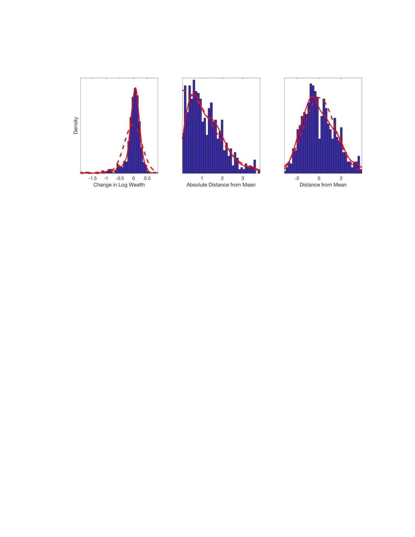
4.7 Tables and Figures

Figure 4.1: Wealth dynamics in the pooled data

Notes: Figure depicts three distributions capturing wealth dynamics at the pooled data.

The solid red line depicts the empirical distribution using kernel smoothing and the

dashed line represents the normal distribution fitted to the data. For the second figure, the

right half of a normal distribution, as absolute values are all positive. All figures use a log

wealth scale on the x-axis and the density on the y-axis. The first graph depicts the

change in log wealth. The middle graph captures the absolute distance of an observation

from the mean, taking into account both x and y distances. The right graph depicts the

distance from the mean with negative values indicating the x-value is less than the mean

x-value.

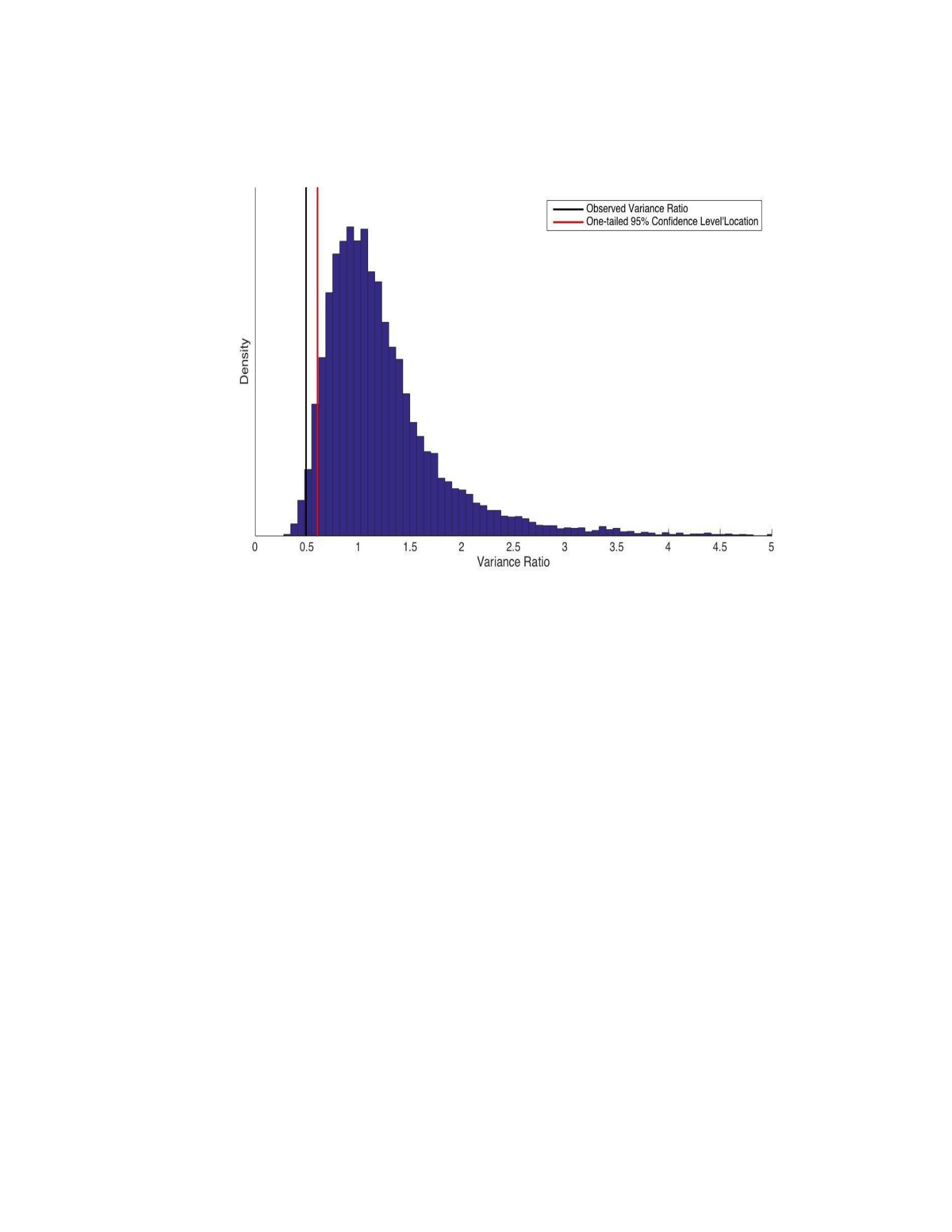
Figure 4.2: Distribution of estimated variance Ratios for an individual

Notes: Figure depicts the density of the simulated variance ratios for an individual. The

vertical red line represents the one-tailed 95% confidence interval and the black vertical

line is the observed variance ratio for the individual. The observed variance ratio lies

below the 95% percent confidence interval indicating we reject the null hypothesis of a

random walk in favor of mean reversion for this individual. Variance ratios are calculated

for comparing a two period lag,





, to the one period lag.

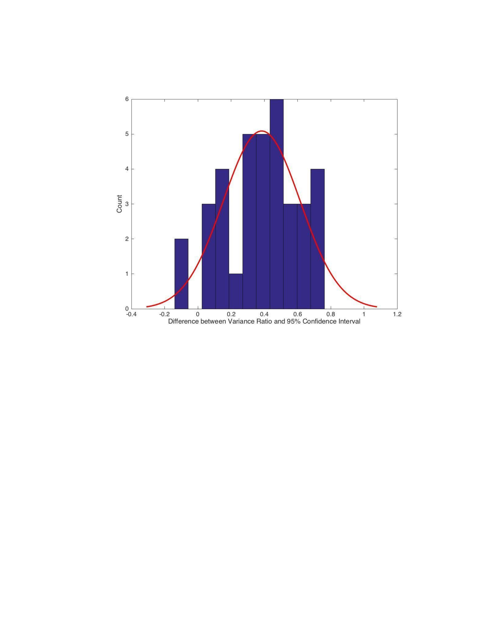
Figure 4.3: Difference between observed variance ratio and one-tailed 95%

confidence interval for all individuals

Notes: Figure depicts the difference between the observed variance ratio and the one-

tailed 95% confidence interval for the 39 individuals with the full 17 periods of wealth

observations. The red line depicts a normal distribution fitted to the data. Observations

below zero indicate a rejection of the null hypothesis changes in wealth follow a random

walk in favor of mean reversion. We reject the null for two individuals out of the 39 total,

which is nearly identical to the 5% we would expect to observe by random chance.

Variance ratios are calculated for comparing a two period lag,





, to the one period

lag.

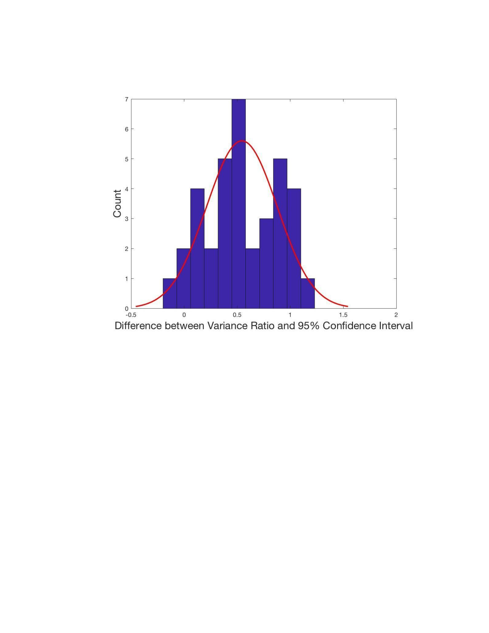
Figure 4.4: Difference between observed variance ratio and one-tailed 95%

confidence interval excluding famine years

Notes: Figure depicts the difference between the observed variance ratio and the one-

tailed 95% confidence interval for the 39 individuals with the full 17 periods of wealth

observations. We exclude timer periods prior to 1986 to remove the famine years. The

red line depicts a normal distribution fitted to the data. Observations below zero indicate

a rejection of the null hypothesis changes in wealth follow a random walk in favor of

mean reversion. We reject the null for two individuals out of the 39 total, which is nearly

identical to the 5% we would expect to observe by random chance. Variance ratios are

calculated for comparing a two period lag,





, to the one period lag.

Table 4.1: Wealth summary statistics by village

Mean Log Wealth

Standard Deviation

Observations

Village 1

95.24

130.48

208

Village 2

82.56

110.22

206

Village 3

55.66

57.47

197

Village 4

41.94

35.61

223

Notes: Table shows summary statistics for wealth for each village. We see substantial

differences in mean herd sizes across villages, which indicates different conditions across

villages.

Table 4.2: Observed mixture fits for the pooled data and for each village

Panel A: Pooled (n=49)

AICc

BIC

ICL

1 Component

4185.60

4204.00

2426.74

2 Components

3514.16

3555.65

2585.37

3 Components

3114.62

3179.29

2711.34

Panel A: Village 1 (n=13)

AICc

BIC

ICL

1 Component

1187.52

1200.56

600.28

2 Components

956.80

986.47

622.57

3 Components

879.50

926.18

649.87

Panel B: Village 2 (n=12)

AICc

BIC

ICL

1 Component

1042.25

1055.24

527.62

2 Components

845.77

875.34

541.72

3 Components

773.25

819.79

600.35

Panel C: Village 3 (n=11)

AICc

BIC

ICL

1 Component

938.81

951.24

475.62

2 Components

737.77

766.14

494.37

3 Components

650.13

694.89

514.90

Panel D: Village 4 (n=13)

AICc

BIC

ICL

1 Component

908.43

921.79

460.89

2 Components

697.95

728.30

507.04

3 Components

613.86

661.57

543.77

Notes: Table presents the information criterion AICc, BIC and negative ICL for fitting

mixture models with one, two and three components respectively. We present the

negative ICL for ease of interpretation, as the proffered model for each criterion is the

minimum value within the column, which is presented in bold font. We reliably find

AICc and BIC to prefer a three-component mixture, while ICL prefers one for the pooled

data and for each village.

Table 4.3: Mixture fits for simulated 2-component model

Panel A: Pooled (n=49)

AICc

BIC

ICL

1-Component

2-Components

0.895

3-Components

0.105

Panel A: Village 1 (n=13)

AICc

BIC

ICL

1-Component

0.984

2-Components

0.77

0.997

0.016

3-Components

0.23

0.003

Panel B: Village 2 (n=12)

AICc

BIC

ICL

1-Component

0.921

2-Components

0.774

0.999

0.079

3-Components

0.226

0.001

Panel C: Village 3 (n=11)

AICc

BIC

ICL

1-Component

0.959

2-Components

0.725

0.999

0.041

3-Components

0.275

0.001

Panel D Village 4: (n=13)

AICc

BIC

ICL

1-Component

2-Components

0.781

0.997

3-Components

0.219

0.003

Notes: Table presents the percentage of times AICc, BIC and negative ICL fit mixture

models with one, two and three components respectively for simulated data with a two-

component model. Parameters for the simulated data come from the 2-component

mixture fit for the pooled data and villages respectively. We find AICc and BIC perform

well at fitting the two component mixture, when it exists, with AICc being more prone to

over fitting the number of components. We find ICL consistently fits the one-parameter

model, indicating it does not perform well at identifying the two-component mixture.

Additionally, we present the number of households in each sample, which we label n.

5. Conclusion

In this dissertation, we investigate poverty alleviation strategies and their outcomes to

shed light on how to optimally provide aid. Optimal aid needs to take into account not

only the underlying cause of poverty and associated underlying asset dynamics, but also

identify potential spillovers aid may have. Understanding the context of poverty in terms

of the socio-economic and environmental contexts is critical in order to ensure poverty

alleviation is performing effectively. We focus on rural populations in eastern Africa,

specifically Tanzania and Ethiopia.

Using a CCT conducted in Tanzania designed to increase health and education

outcomes as well as provide poverty relief, we find there is an increase in both direct

fishing pressures from additional households earning money from fishing due to program

participation as well as an increase in demand for seafood. Both put increased pressures

on local fisheries indicating this poverty reduction policy may have negative spillovers in

terms of local fisheries. While we do not go as far as to say this policy is sub-optimal

because of these spillovers, we stress the importance of identifying spillovers and

planning for them when combating poverty.

The results from chapter two are insufficient in themselves to determine if the

spillover into the fishery sector is a negative impact. The other part needs to be to

determine if local fisheries are at risk of overfishing. Understanding the complete picture

of the nexus between the environment and the socio-economic system is essential to

understanding the extent of how spillovers will impact the long-term wellbeing of the

people in the system. In a study using data up to the year 2000, Berachi (2003) finds

many Tanzanian fisheries have already surpassed their maximum sustainable yield. Thus,

increased fishing pressures both from increased consumption and additional households

using fishing as an income source, are likely to exasperate the issue. Especially in inland

fisheries, even when fish catches are increasing, it is possible to be depleting stocks of

specific fish resulting in a loss of biodiversity and reduction in the sustainability of the

fishery (Allens et al., 2005). The spillover into the fishery sector are not necessarily a bad

thing, especially when fish populations are abundant.

In cases where local fisheries can support additional fishing pressures, the

spillover could be a substantial benefit to the populations. We found the moderately poor

show increased likelihood of entering the fishing industry due to participation in the

CCT. One explanation is these households were able to afford fishing gear and gained

access to an additional revenue stream and means of diversifying income. In other words,

they are able to surmount a Micawber Threshold, which could put them on a higher

wealth trajectory resulting in long-term reduction in poverty. Regardless of the state of

fisheries, it is important to consider how poverty reduction policies may impact the

fisheries in order to manage the fishery in a sustainable manor. A change in aid policy

may need to be accompanied by changes to how nearby fisheries are managed in order to

maximize the benefit of the aid program and minimize the negative spillovers to the

fishery sector.

Next we present a poverty trap model based loosely on the pastoralist system of

the Borana Plateau in southern Ethiopia and use numeric simulation to determine optimal

level of aid. We identify a range of inefficient aid levels below the Micawber Threshold,

which we define as the inefficient aid trap. This region is characterized by higher rates of

poverty and higher costs due to individuals being held at an unsustainable wealth level.

Thus, the Micawber Threshold is a lower bound for optimal aid level and that aid should

be set significantly above the estimated Micawber Threshold when there is uncertainty of

the location of the Micawber Threshold to avoid the aid trap. Additionally, we find the

coupled relationship between level of poverty and cost ensures the cost of poverty

alleviation is the primary driver of optimal aid and the social cost of poverty is a

secondary concern. These results hold for multiple equilibrium poverty traps where

households have homogenous dynamic wealth equilibria. We leave it for future research

to determine if this changes when we allow for heterogeneity amongst individuals. Initial

steps would be to use a more complex poverty trap model in line with Ikegami et al.

(2016), which allows for heterogeneous individual ability and apply a basic wealth policy

to these individuals. Additionally, the model would benefit from explicitly modeling the

intertemporal choice problem of individuals to include consumption and savings

decisions to determine if the ability to asset and/or consumption smooth impacts the

results of our basic model.

Lastly, we introduce a novel test to identify multiple equilibrium poverty traps.

We provide a falsification test by identifying mean reversion at the individual level using

a variance ratio test. This test surmounts two major issues associated with identifying

multiple equilibrium poverty traps: few observations near the Micawber Threshold and it

allows for heterogeneous equilibria across the population. Our second test utilizes a

mixture model to identify clustering in the aggregate and village level data. This is a

weaker test, as it still requires assuming homogeneous wealth equilibria. We find no

evidence using a data set, which was previously used to identify a multiple equilibrium

poverty trap. This highlights the importance of rigorous tests to ensure we know the

underlying cause of poverty to ensure we combat it appropriately.

The empirical difficulty of identifying multiple equilibrium poverty traps has

important implications for the theoretic model of combating poverty traps described in

chapter 3. First, it is extremely unlikely that poverty traps exist where there is a unique

and stable Micawber threshold for all individuals within a population. Even in the

relatively simple environment of the Boran pastoralists, it is difficult to identify a unique

Micawber threshold within a village, much less across the sample as we show in chapter

4. When more diverse livelihoods are available, which is the case in most contexts, this

problem is exasperated. Thus, finding a unique Micawber Threshold to use as a target for

aid policy is unlikely to be appropriate. However, our finding of asymmetric costs of

incorrectly targeting aid still has important policy implications even when heterogeneous

Micawber Thresholds exist.

Rather than looking at our results in terms of an overarching policy, we can think

of it in terms of each individual. As there is a much larger cost for underproviding aid to

any individual, when Micawber Thresholds are heterogeneous providing a basic wealth

policy should be placed towards the upper end of the distribution of individual Micawber

Thresholds. For instance, assume two individuals with heterogeneous Micawber

Thresholds (similarly you could think of two groups of individuals with each group

having a unique Micawber Threshold). Targeting a basic wealth policy at the average of

the two Micawber Thresholds would clearly be inefficient as increasing the level would

reduce the cost of providing aid as the cost of providing aid is much higher when aid is

set below the Micawber Threshold compared to an equal amount above it. This inference

is similar to the case of an uncertain Micawber Threshold, where erring on the side of

overproviding aid is preferable when combating multiple equilibrium poverty traps.

An alternative approach to combating multiple equilibrium poverty traps

heterogeneous Micawber Thresholds could be using insurance. This would benefit from

not having to identify individual Micawber Thresholds, as individuals would be able to

determine when and how much insurance to purchase based on their experience and

conditions. The issue with insurance is those closest to the Micawber Threshold, i.e.

those who would benefit most, are least likely to purchase insurance as the cost may

place them below the Micawber Threshold (Janzen 2012). Insurance would only be

effective with substantial subsidies designed to allow those near the Micawber Threshold

to invest in it.

Future work concerning exactly how to incentivize this while minimizing the

issues of the moral hazard problem would improve the effectiveness of this approach.

The goal would be to allow individuals to insure up to their individual Micawber

Threshold or, potentially, slightly above it at a rate far below the fair insurance price.

However, if they desire insurance above this level, the price should rise approaching the

fair price. However, this would either require extensive cost to identify individual

Micawber Thresholds or accepting some level of providing aid in the form of insuring at

a higher level than the Micawber Threshold for individuals with relatively lower

Micawber Thresholds. While potentially costly, this additional insurance would be a form

of aid, which would effectively provide a safety net and protect individuals from falling

into the poverty trap region and when set at reasonable levels near the upper end of the

Micawber Threshold distribution, may represent significant improvement in efficiency

for society. Determining the appropriate level of insurance and how to discount it should

be done as future work through numeric simulation and ideally a randomized control trial

implementing a subsidized insurance program to test its effectiveness.

Insurance by itself would only work as the safety net portion of a program. This

will need to be combined with some form of cargo net to bring individuals up to their

respective Micawber Thresholds. This is especially important for situations where the

low production technology draws upon a local public good, such as in the case of the

Boran pastoralists. Failing to bring herd sizes up to the point where they can engage in

mobile pastoralism may put additional pressures on the local pasturelands exasperating

the tragedy of the commons (Lybbert et al., 2004). This potential spillover into the

natural resources available is similar to what we explored in chapter 2. If aid is set too

low where households are able to maintain their local warra herd, but not large enough

for to keep a mobile fora herd may result in additional overgrazing and a reduction of

productivity. This environment-poverty trap would put additional pressures on the

already fragile ecosystem and cause additional dependence on external aid resulting in an

aid trap.

Utilizing conditional cash transfers may help to ensure this does not happen. If aid

requires any cattle purchased (similarly the transfer could be in the form of livestock)

would have to be grazed away from the village, this would reduce the likelihood of

localized overgrazing. This condition may require households to pool herds, which is

atypical for these populations. This would run the risk of imposing restrictions that go

against culture and tradition and should be discussed at lengths with village leaders

before attempting to implement. This is especially important because how linked status is

with one’s herd. However, changing conditions may necessitate the shifting of cultural

norms in order for the pastoralism of the Borana Plateau to remain viable. Changes still

need to come from within rather than being forced upon them by outside agencies in

order to ensure the important aspects of the local culture remain intact and that aid is

received and utilized by the pastoralists.

Another form of aid to consider for the pastoralists is providing access to

microfinance, which could act as both a form of cargo net and safety net. Providing loans

to allow households to surmount their personal Micawber Thresholds would allow for

households to put themselves on a path of wealth accumulation, allowing them to pay

back the loans in future periods. Alternatively, during bad periods households would have

the option to take out loans rather than draw down the productive assets of the herd

allowing for more effective consumption smoothing without the risk of falling below the

Micawber Threshold.

A major downside to microfinance is the asymmetric information between

borrowers and lenders results in the adverse selection and moral hazard problems (Udry,

1994). A common solution used in rural microfinance has been to use joint-liability

contracts placing the liability of individual loans on the whole group (Marr, 2012). This

would utilize social pressures to help ensure loans are repaid when able. However, much

of the risks associated with the Boran pastoralists tend to be systematic, such as drought

affecting much of the plateau, which may reduce the effectiveness of these joint loans

during bad years, which would increase the cost of providing loans and, in turn,

increasing the price for the pastoralists. It may be desirable to combine this with some

kind of index-based insurance program, potentially funded through government aid

programs, to reduce the risk of the majority of loans failing for a village, thus reducing

the risk of the lenders. This combined policy would remove much of the moral hazard

and adverse selection issues, while still providing additional aid during drought years.

Regardless of the form the aid takes, when multiple equilibrium poverty traps are

present it is critical to ensure individuals are able to surmount the critical Micawber

Threshold and to protect assets from falling below this level in future periods. The goal of

aid is to both enhance current wellbeing and, perhaps more importantly, to enable

households to maintain a high-level of well being in future periods. Enabling self-

sufficiency rather than building a reliance on aid programs resulting in the aid trap is

critical to ensuring aid budgets can be used to create the most benefit possible. Short-term

thinking of trying to reduce current payments may be contrary to this goal of creating

sustainable growth if aid is provided short of the Micawber Threshold.

Together these chapters stress the importance of identifying the cause of poverty,

understanding the underlying wealth dynamics leading to poverty, and identifying any

spillovers of aid policies in order to design effective aid strategies. Failing to do any of

these may potentially lead to undesirable outcomes depending on the context. We hope

these results can be built upon and used in the future to provide better aid to

impoverished populations to help make the dream of eliminating extreme poverty a

reality.

Students also viewed