Unlocking the potential of Earned Value management in construction: A Comparative Study

Chapter 1: Introduction

1.1. General Introduction

To monitor the project is to compare the current with the planned situation, determining if the

costs and the schedule are progressing according to plan, in order to take corrective action when

needed. Any project with a considerable cost overrun and schedule delay typically gets in

trouble at its beginning as indicated by Alvarado (2004). In addition, project managers do not

realize this problem until late in the project when their ability to recover the project to achieve

its planned objectives diminishes.

EVM is the most used multi-dimensional project control method, as it integrates time

and cost (Rozeneset al., 2006). The Project Management Body of Knowledge (PMBOK)

defines control as “comparing actual performance with planned performance, analyzing

variances, assessing trends to effect process improvements, evaluating possible alternatives,

and recommending appropriate corrective action as needed.” (PMI, 2004, p. 355). In another

study evaluating the reliability of EVM conducted by Mahdi et al. in 2016, it was discovered

that among the EVMs assessed in the sample cluster, time schedules were identified as the

most influential. Additionally, the study noted that while quality also played a role, its impact

was not as substantial as the time schedule, yet still considered significant. Keeping under

budget and ahead of time schedule are key measures for project success. The executed work

compared with planned work is considered a work performance indicator, also the cost spent

compared with the cost remaining can be taken into consideration as a work performance

indicator. DE Marco et Timur, (2013) stated that indicators are essential management tools in

monitoring and evaluating project activities, as they allow the achievement of goals to be

monitored as well as advances and improvements in quality to be identified.

The EVM method has been used for numerous projects during the past 40 years (Lipke,

2008). This method had a favorable impact on various aspects associated with project

outcomes, including but not limited to enhanced planning, risk evaluation, monitoring,

reporting, and controlling. Nevertheless, few researchers have shown some studies regarding

the analysis and evaluation of time and cost performance stability while taking into account the

quality of work. Despite the fact that EVM has been employed by numerous companies for

over 35 years as a means to forecast time and cost outcomes, numerous studies, including

(Lipke et al, 2009), have identified weaknesses in its effectiveness.

The evaluation of project performance involves analysing earned value indicators

related to cost, schedule, and scope. These aspects, are known as the iron triangle as recognized

by the Project Management Institute (PMI), are crucial for ensuring project efficiency (Project

Management Institute, 2017). To derive the earned value indicator, it is imperative to quantify

activities in terms of cost and establish completion dates for each task. As highlighted by

Vargas (2003), the EVM technique intricately links cost, schedule, and scope in project

management.

1.2. Problem Statement

Since the development of EVM, the implementation of this approach is yet questioned in the

construction industry in Egypt and potential improvements are yet on the verge. There are

various studies in the literature review that discussed the potential limitations of EVM and the

urgency of further investigation to enhance the process and outcomes of using EVM in the

project (Mahdi et al., 2018). Some of the limitations were the complexity of the process, lack

of sufficient accuracy, and the process is classified to be time-consuming (CanCandido et al.,

2014). Therefore, with the current advancement in the tools and technology used in the

construction sector, there is a prospective opportunity to invent well controlled EVM approach

that can improve the overall management of the project regardless of its circumstances and

challenges.

Luis Felipe Cândido et al. (2014) investigated conceptual problems and implementation

difficulties associated with EVM. Through a case study on a construction project utilizing

EVM for planning and control, they identified four major issues. The EVM approach, they

found, falls short in supporting lean construction applications. Two notable problems include

the neglect of the mobilization of resources phase and the absence of consideration for

construction indirect costs. In their conclusion, the researchers asserted that EVM merely

extends the traditional approach of measuring physical and financial progress over time. This

narrow approach is insufficient to provide a comprehensive managerial tool, as became clear

through the analyses of the building project under consideration. The main advantage of this

technique is its relative simplicity and that it only requires the kind of information (activity

percentages of completion and actual costs mostly) that is gathered for other purposes during

the project execution. The biggest disadvantage, which has apparently remained out-of-sight

for most practitioners and researchers alike is that EVM is a technique that measures ‘amount

of work performed’, not time deviations.

Put it in simple words, EVM measures the differences between earned value (EV) and

planned value (PV) (for time deviations) or between EV and actual cost (AC) (for cost

deviations). If EV is greater that either PV or AC, the project is doing well in time or cost,

respectively. But EV increases as more activities are finished, irrespective of whether the order

of execution was the most appropriate. The reasonable question then is: are the activities being

finished so far, the ones that will lead to achieving the project duration we planned originally?

EVM cannot tell. Indeed, if we deviate significantly from the project schedule, complementary

indices like the p-factor (Lipke 2004), which measure schedule adherence, inform us about the

risk of rework but they still fail to anticipate what (negative) time deviations can be expected.

EVM is therefore, a technique that works perfectly in the cost dimension (Ballesteros-

Pérez et al. 2015, Ballesteros-Pérez et al. 2016), as all activities contribute to the total project

cost according to their respective budgets. But that is not the case for time deviations. Activities

need to happen in specific order to achieve a particular duration. According to Fleming and

Koppelman (2010), EVM techniques are difficult to be applied to dynamic construction

projects and do not add much value to project execution, especially when: 1) There is absence

of adequate project planning and documentation, 2). The construction schedule is compounded

by considering the resource constraints such as resource availability limits and multiple

calendars, iii. Activity and project delays encountered during project executions, iv. There is

no EVM analyst or specialist within the project team. Some problems that may impede the

implementation of EVM as specified by Kim et al. (2003) such as: - High cost, complicated

and burdensome paperwork - Poor understanding of EVM - Distrust and conflict between

project managers, project consulting and government -Pressures to report only good news.

The critical need for effective earned value techniques in the construction industry,

specifically focusing on project forecasting accuracy across diverse construction projects in

Egypt Furthermore, the variation in the most accurate technique based on project type and

duration introduces complexity in selecting the optimal method. Renovation and residential

projects favor the Earned Schedule method, while industrial, commercial, and educational

projects consistently lean towards the Earned Duration method. This inconsistency prompts the

need to identify a systematic approach for method selection tailored to specific project

characteristics.

In essence, the problem revolves around reconciling the overall effectiveness of the

Earned Duration method with the nuanced performance variations under different performance

factors and project types. The challenge is to provide a comprehensive and applicable

framework that assists project managers in selecting the most efficient earned value technique

for precise project forecasting, considering the unique characteristics of each construction

project in the Egyptian context.

1.3. Research Goal and Objectives

The goal of this research is to enhance the application and accuracy of earned value techniques

in Egyptian construction projects through a comprehensive evaluation of Earned Duration,

Earned Schedule, and Planned Value methods. The research seeks to understand variations in

technique accuracy based on project type, particularly focusing on preferences for specific

methods in different project categories. Key goals include developing a systematic approach

for selecting the most accurate technique, assessing and refining practical guidelines for

decision-making, and exploring the impact of performance factors like SPI and CPI.

Ultimately, this will promote the adoption of earned value techniques for improved project

forecasting in the Egyptian construction sector.

The objectives of this research are the following:

1. Evaluate the effectiveness of earned value techniques in forecasting project completion dates

across diverse construction projects in Egypt.

2. Investigate the variations in the accuracy of earned value techniques based on project type

and duration, specifically examining the preference for the Earned Schedule method in

renovation and residential projects and the consistent preference for the Earned Duration

method in industrial, commercial, and educational projects.

3. Develop a systematic approach for selecting the most accurate earned value technique

tailored to specific project characteristics, aiming to address the complexity introduced by the

varying preferences for techniques across different project types.

4. Assess the practical guidelines introduced in the thesis for choosing the most efficient

technique based on project duration percentages.

5. Examine the interplay of performance factors, including Schedule Performance Index (SPI)

and Cost Performance Index (CPI) for different project types, to gain a more nuanced

understanding of their impact on the accuracy of earned value techniques.

6. Develop a comprehensive and applicable framework that reconciles the overall effectiveness

of the Earned Duration method with nuanced performance variations under different

performance factors and project types, aiming to provide practical guidance for project

managers in the Egyptian construction context.

1.4. Research methodology

The proposed methodology of this research will rely on a methodology that involves

quantitative data analysis. The first step involves reviewing different techniques to measure

earned value management. These different techniques will be reviewed comprehensively in the

literature part. A comparison between the different techniques will take place in order to

differentiate between each of these techniques in addition to highlighting their major

differences. These techniques will be applied on numerous construction projects in Egypt in

order to evaluate their efficiency based on different factors such as project type, total price,

project duration and deviations between planned and actual cost and time. Analysis of the

accuracy of these techniques will take place to determine which of these techniques fits and

give more accurate results. In order to define the accuracy of each method, a numerical analysis

will be conducted as a quantitative approach. Finally, based on the findings of the analysis, a

model will be established to estimate the forecasted finish date. Details of the research

methodology are described in Chapter 3, in addition figure one below illustrates the sequence

of the research methodology.

Figure 1 Research Methodology steps

1.5. Expected significance of the research

The research is anticipated to significantly contribute to the construction industry by enhancing

project forecasting accuracy. The identification of the most effective earned value techniques

for different project types and durations, as highlighted in the thesis, is expected to provide

project managers with valuable insights to improve the precision of their forecasts.

The research's emphasis on tailoring the choice of earned value techniques to specific

project characteristics is expected to be a valuable contribution. This tailored approach is

anticipated to empower project managers to make informed decisions based on the unique

requirements and dynamics of each construction project, fostering more efficient project

management practices.

The practical guidelines introduced in the thesis for choosing the most efficient technique based

on project duration percentages are expected to provide clarity in decision-making. Moreover,

the research's nuanced understanding of the interplay of performance factors, including SPI

and SCI, is anticipated to offer practical insights, enabling project managers to navigate

complexities and optimize forecasting accuracy, with a special focus within the Egyptian

market.

1.6. Thesis Organization

This document is organized into six chapters, each serving a distinct purpose in the

exploration and analysis of EVM in construction projects.

Chapter 1 provides a comprehensive overview, starting with a general introduction to

the research topic. It includes a clear statement of the problem, articulation of the research goals

and objectives, an explanation of the chosen research methodology, and an overview of the

expected significance of the study.

The second chapter is dedicated to the literature review, offering a thorough

examination of background information on the subject, an exploration of various EVM

methods, and a review of relevant previous studies. This chapter serves to establish the context

for the current research and identify gaps in existing knowledge.

Chapter three details the research methodology employed in this study. It outlines the

chosen data collection methods and elucidates the data analysis techniques applied to scrutinize

the collected information. This chapter serves as a roadmap for the systematic execution of the

research.

The fourth chapter delves into the specifics of data collection, providing detailed

information about the projects selected for analysis. This section offers insights into the

variables, parameters, and scope of the data collected for the study.

Chapter five is dedicated to the analysis of the collected data. It presents the outcomes

of the analysis, providing a comprehensive understanding of the research findings.

The chapter six concludes with a summarization of the key insights and implications

drawn from the analysis, marking the end of the research journey.

Chapter 2: Literature Review

2.1. Background

The failure of construction projects in meeting cost and schedule requirement has forced project

managers to find any opportunity to invoke their learning and understand the causes of failure

for future projects (Hughes et al, 2017). In an effort to enhance project management success

rates, EVM has been developed as a tool that managers can utilize to aid in the attainment of

desired client deliverables. EVM has been in existence for some time, and its effective

implementation in projects remains a persistent challenge.

EVM is a project management technique used for improving the rate of success of

construction projects (Aramali et al, 2022). EVM stands as the most extensive approach for

overseeing and managing a project's cost and schedule performance by unifying the project's

scope, budget, and timeframe (Dube, 2018). There are many other sectors that are using the

methodology of EVM such as software industry, space industry, military applications, and

energy sector, and this application still improving and developing widely. Company managers

continually strive to minimize costs in the manufacturing and production processes, a task that

significantly influences their financial management (Villafanez et al., 2020).

The history of EVM dates back to many decades ago and after the second world war.

The critical path method (CPM) was introduced in the 1950s as a technique for assessing and

enhancing performance. The US navy then invented the idea of using project evaluation review

known as (PERT). PERT was established in a manner akin to CPM, and it served as a precursor

to the development of EVM. After that, in 1960’s the US government invented the idea of

EVM to be used in their projects and measure their performance (Nevison and Chichakly,

2021). The establishment of the Project Management Institute in 1969 marked the initial

significant milestone in the evolution of project management into a recognized profession

(Kabeyi, 2019). The inception of project management functions enabled managers to discover

practical solutions to project limitations.

EVM does not exclusively concentrate on the critical tasks of the project. It can involve

all types of tasks (i.e., non-critical tasks, and critical tasks), whilst the critical path of the project

is still considered essential to estimate the total time required to complete the project. The

critical path comprises a continuous sequence of activities with no slack, and these activities

are referred to as critical tasks. This indicates that controlling and monitoring the schedule of

work in the project can concentrate on these main tasks as no delay can be allowed because

any delay in these critical tasks can lead to the overall project delay (Corovic, 2022). Many

tasks are allowed to finish late during the execution of the project. Nonetheless, the traditional

earned value method would fail to detect these delays, and the schedule management indicators

would indicate an ideal value even following the postponed task (Schedule performance index

of one, or schedule variance of), which might not be the case (Corovic, 2022). EVM is helpful

in accurately estimating savings and cost overruns in the execution of construction projects.

Nevertheless, employing this approach for overseeing and managing schedule deviations is

insufficient.

The utilization of EVM across all project levels enhances the likelihood of success by

granting project managers the flexibility to make necessary adjustments for achieving success.

EVM can be a short-term method that helps the project manager to measure and control the

performance of the project after the inception stage and report anything related to the time and

cost of the project (Mogaji, 2019). Earned Value Management Systems (EVMS) equip the

project management team with software, procedures, instruments, and project templates to

enhance project success rates. EVMS is an EVMS that aligns with the EIA-748 EVMS

guidelines.

EVM tries to combine three correlated element of project performance, these are the

cost, schedule, and scope (Geneste, 2019). The assessment method known as earned value

analysis (EVA) empowers the project manager to employ a quantitative approach to gain a

deeper insight into project performance. This is achieved by calculating schedule and cost

variances throughout the project's duration. When the project manager finishes around 20% of

the project, the rest of the performance may result in an estimation of around 10% plus or minus

any variation. Project managers can utilize the information provided by EVM for trend analysis

and forecasting, making it a valuable tool for cost control measures. With its robust predictive

capabilities, EVM offers project managers an effective approach to project management.

Project managers can gain many benefits and advantages of utilizing EVM in their

project management methods and to be used for measuring and evaluating the performance of

their projects. EVM can provide stakeholders with transparent metrics, visibility, and clearly

defined accountability. This technique can be excellent for managers in offering an

unobstructed understanding of the project with an overall view of its performance starting from

the inception stage and can still be effective and efficient with many project stages and at all

levels. The procedure enables the project manager to take action proactively, making

adjustments to the project scope and budgets, seeking additional resources, and managing

customer expectations, all before a crisis arises. A database can be developed by project

managers to help in taking many actions and assist in various aspects in the project including

proper decision making for projects in the future and align their progress and work with

unknown risks to be reduced in future projects and ensure the prevention of any cost overrun

especially from risks that were considered critical in the past and had severe impact.

Furthermore, and of utmost significance, managers can employ the tool to conduct a

comparison and establish benchmarks for the current project status when compared to the

project's initial baseline. Additionally, they can pinpoint the critical path. Mogaji (2019)

indicated that a basic technique of EVM in a construction project can help project managers

with an adequate and accurate estimation and forecasting of around 20% of completed works

in the project. There are many quantitative equations and formulas that are currently available

to improve the performance of construction projects.

2.3. Earned Value Management

The traditional approach of managing changes in the project involves comparing the gap

between the actual variable value and the planned value. As an illustration, it is possible to

analyze the real accumulated project costs in comparison to the initial projected project costs

to identify variances in the project's expenditure (Buestan et al, 2018). Nonetheless, this

examination is partial because it's possible to have expended 90% of the budget while only

completing 50% of the project. The traditional cost analysis techniques do not determine the

status of the project and whether it is being performed properly, since the information about

the execution of the project is not available (Buestan et al, 2018).

In the traditional approach, a couple of variables are compared with each other; the

budgeted cost of the planned activities, known as the planned value (PV), and the actual real

cost of the performed activities known as (AC) (Aramali et al, 2021). The planned value (PV)

is linked to and symbolizes the project schedule in monetary terms, while the actual value (AC)

is tied to the actual cost of the project in monetary units. This comparison neglects completely

the scope of work which can be the third variable in the equation and a major constraint in

construction projects (Aramali et al, 2021). This is accomplished by means of the earned value

(EV) or the cost of work performed as budgeted, both of which are related to the project's scope

variable in terms of monetary units (Aramali et al, 2021).

The concept of earned value is generated from the idea that every delivered project has

a budgeted cost known as the value. When the cost of the project is well delivered, it indicates

that the value is well earned. EVM integrates the three pertinent project baseline factors: scope,

timetable, and financial plan (Zahoor et al, 2022). It is important to calculate many factors

such as the earned value correlated with the scope of work in monetary units, the planned value

correlated with schedule of work in monetary units, and lastly the actual cost of work in the

project again in monetary units (Zahoor et al, 2022).

The budget cost at completion indicates the baseline cost for the project and the initial

budget required in order to plan the performed work on site. It can be represented on the S

curve of the project accumulating the expected cost of each task during the whole life cycle of

the project. It signifies the anticipated value of all tasks and activities that are scheduled to be

finished (Mayo-Alvarez et al, 2022). The budget cost at completion (BAC) can be calculated

through the planned value as shown in equation 1:

𝑃𝑉 = 𝐵𝐴𝐶 ∗ 𝑃𝑊

Equation 1 planned value (Mayo-Alvarez et al, 2022).

Where:

 PV: Planned value

 BAC: budget cost at completion

 PW: planned work percentage

The other major variable in the EVM is the earned value (EV), which refers to the budgeted

cost for the performed work It represents the projected cost, based on the budget, to complete

the work that has been executed within the specified timeframe, rather than the actual cost. It

helps in understanding the work performed until a specific date and the budgeted value, it can

be calculated through equation two.

EV = BAC × WD

Equation 2 Earned Value (Mayo-Alvarez et al, 2022).

Where:

 EV: Earned value

 BAC: budget cost at completion

 WD: work done percentage.

The actual cost is the incurred budget that was used for the performed work until a certain

date (Mayo-Alvarez et al, 2022). This is the real-time cost of the work, encompassing both

direct and indirect expenses. It provides insight into the total cost incurred for the work

completed thus far. Its value is calculated as the sum of (quantities completed multiplied by the

actual purchase price) (Mayo-Alvarez et al, 2022).

EVM is very valuable when used to compare the cost gaps of the project using cost

performance index and cost variance indicators. These indicators can demonstrate if the project

is suffering from cost overrun or achieving cost savings. The standard variance can be used to

estimate the measurement of deviations in the schedule of work in the project and help in

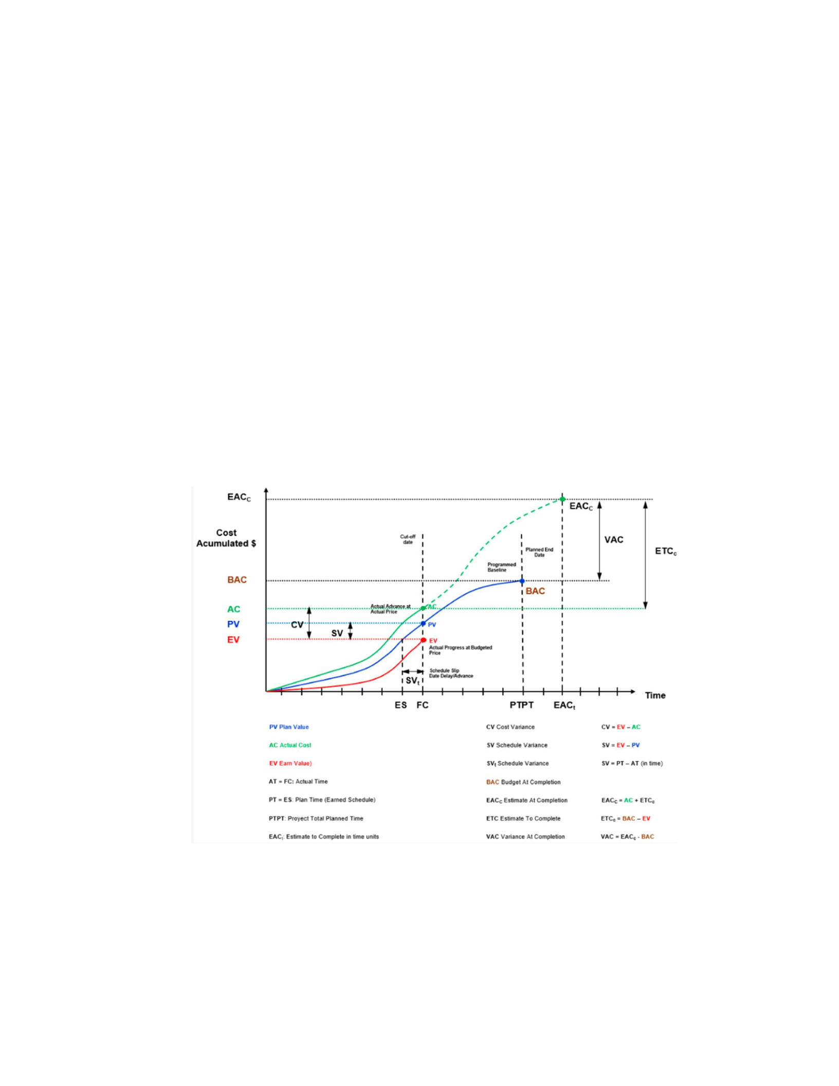
indicating the delay or project overruns (PMI, 2011). Figure 1 depicts the three curves related

to PV (Planned Value), EV (Earned Value), and AC (Actual Cost), along with the cost and

schedule variances measured in monetary units. Employing this method to monitor project

schedule deviations may not effectively handle various project scenarios and does not utilize

time units to report project progress or delays (PMI, 2011).

Figure 2: Earned Value Management: The three curves and cost and schedule variations (Mayo-

Alvarez et al, 2022)

2.3.1. Earned Schedule

The earned schedule is basically the actual progress of work in the project valued or represented

in time units (Lipke, 2012). The commonality between earned schedule and earned value is

that they both utilize actual progress as their initial reference point (Kapuganti et al, 2019). The

major variation between them lies in how expressing and showing the actual progress on site.

Nevertheless, earned programming demonstrates the actual progress of work in the project in

time unites, while the earned value demonstrates the actual progress in monetary figures

(Henderson, 2005). The earned schedule method produces metrics that accurately gauge the

project schedule's status throughout its entire life cycle. This approach enables the assessment

of project progress or delays in terms of "time" units and effectively identifies and quantifies

delays in activities that have been completed behind schedule (Henderson, 2005). Therefore,

earned schedule helps to reduce two major limitations faced when using EVM as a method of

project control (Henderson, 2005). The next figure indicates the earned schedule basic

definition, where the earned schedule value is accomplished when the earned value on the

control date is the same as the planned value in 9 months.

Figure 3: Basic illustration of the idea of earned schedule (Mayo-Alvarez et al, 2022)

The earned schedule is similar to the EVM in the case of plotting S curve as a

representation and a reference for the schedule variation, but it does not differentiate between

the non-critical activities and the critical ones (Capone and Narbaev, 2021). This particular

aspect renders the accuracy of schedule variance measurement questionable because it suggests

that only critical path tasks should be taken into account when overseeing the project's timeline

(Capone and Narbaev, 2021). Therefore, the critical path earned scheduling (ESRC) was

developed to integrate the idea of earned schedule and critical path of the project and overcome

the limitation of the original concept. To achieve this, it is essential to establish and utilize the

S curve specifically for critical tasks as a benchmark to estimate schedule deviations (Capone

and Narbaev, 2021).

2.4. Previous Studies

Bhosekar and Vyas (2012) studied the cost control of construction projects using EVM. The

study concentrated more on the real estate sector. The study delved into the significance of the

EVM tool, explored its fundamental formula along with performance indicators, and applied it

to a case study involving a residential building covering an area of 120 square meters. This

case study was used to conduct EVM analysis, tracking both time and cost indicators. To

compare EVM analysis with software like MSP, P6, and SQL, the author compared multiple

project management tools. Additionally, the paper concludes with a comparative analysis of

EVM Analysis in contrast to various other management tools.

Virle et al (2013) discussed the implementation of both EVM and Earned Schedule

(ES) in construction projects. In this study, the researcher explored the utilization of EVM in

the construction sector, discussed the elements of EVM, and outlined the various parameters

impacting the significance of ES and EVM.

Gaddam and Landage (2022) reviewed the utilization of earned schedule and EVM for

construction projects. Project success is heavily reliant on achieving the anticipated cost and

time of construction projects. Public and private sectors have a long history regarding the

inability of completing projects on time and cost. Earned schedule and value management are

two methodologies used in project management for organizing and monitoring the progress of

work in the project. These methods are extremely useful in comparing the actual cost of work

and the budgeted one while considering the analysis of schedule delays. EVM is quite efficient

method for controlling and evaluating construction projects. It can be used by stakeholders,

project managers, and most parties to visualize the progress of the project during its entire life

cycle and allow the team to properly manage the project. On the other hand, earned schedule

is more about the practical knowledge that builds the idea of EVM. It is now considered the

newer extension to the concept of EVM. To enhance the control and evaluation of schedule of

work and performance during the life cycle of the project, earned schedule allows EVM to

convert its outcomes into time metrices. Project manger’s performance can be comprehensively

improved with earned schedule by forecasting and making better decisions in the project. The

aim of this research was to apply the concepts of earned schedule management and EVM to a

flyover infrastructure construction project in India to evaluate cost overrun and time delay. The

results were then compared with the outcomes of using MSP software predictions. Study’s

findings demonstrated the ability to use ES and EVM to monitor and control the time and cost

of infrastructure projects efficiently and accurately. It can aid in predicting early warning of

variances in the time and cost using ESM and EVM parameters during the whole life cycle of

the project.

Suresh and Ganapathy (2015) showed a study regarding the implementation of earned

value analysis for evaluating project performance. The study addressed earned value analysis

for examining the performance of construction projects. EVM offers the ability to understand

the cost of construction projects and the impact of the performance, risks, and scope of work

on the cost of projects. It motivates the management team to maintain a keen focus on cost,

time, and progress, thereby facilitating smoother project execution. On the other hand, Chavan

and Bhamre (2015) studied the ability to efficiently plan and schedule residential projects while

conducting a delay analysis. The research focused on many aspects including manpower

organizing, project planning, manpower management, project scheduling, project scheduling

steps, delay analysis, manpower planning, introduction to scheduling, planning steps,

introduction to planning, and other related information. Furthermore, a case study of a

residential unit project was illustrated through the use of MS Project and MS Excel software.

The study concluded with main points regarding the master schedule, planning of activities,

and other topics. The main causes of delay in the project were weather conditions, lack of

skilled labours, improper planning, poor organization, shortage of materials, and shortage of

labours. Therefore, this study indicated the importance of proper planning for the success of

construction projects and avoiding any time spent waiting.

Yvas (2016) tracked the progress of construction projects using EVM. The goal evolved

around demonstrating the efficiency and role of EVM for project tracking and its superiority

over the traditional approaches. EVM can be crucial for cost and delay analysis of construction

projects as proven in this study and agreed by many studies in the literature. Hence, it concluded

with the main benefits of using EVM in the construction industry and project management.

Mayo-Alvarez et al (2022) conducted an AHP systematic analysis of EVM techniques

that are used to control and monitor the performance of construction projects. Successful

management of projects relies on accomplishing the expected objectives. In these goals,

technical achievement is linked to meeting the project's baseline expectations. The project’s

baseline defines lots of information about the project such as the total cost on the S curve, time

of activities, and the work breakdown structure. In simple terms, the project is considered

technically successful when it can deliver its entire scope according to the established schedule

and without incurring additional costs. The baseline performance management helps project

managers to control and monitor the process of activities, costs, durations, and deliverables in

the project. In a conventional method, for projects following a waterfall approach and utilizing

the critical path concept, the primary tool for managing baseline performance effectively is

EVM (EVM). In practice, EVM is well effective for controlling the cost of construction

projects, nevertheless, implementing this technique to estimate the schedule status is usually

inconsistent and not effective. During the past few decades, various changes of the original

concept of EVM have been introduced to overcome this inconsistency when it is applied to

determine and measure the status of project’s schedule and timeline. There are many variations

under the original concept of EVM such as critical path earned schedule, critical path earned

value, the earned schedule, the work in progress earned value, and the critical path earned value

and the work progress combined. Every one of these suggestions aims to rectify certain

shortcomings in the conventional approach of EVM when it comes to time tracking and control.

For instance, they emphasize the importance of focusing on critical tasks for monitoring

schedule progress, addressing the issue of delayed task recognition, reporting schedule

variances in terms of time units, and measuring compliance with the project's schedule (referred

to as the "P factor"). Given the challenging circumstances, it's imperative to identify the most

suitable alternative from various versions of the original earned value method for effective

project schedule management. This selection process involves considering multiple evaluation

criteria. In this research, we conduct a systematic review and comparison of EVM (EVM) and

its variants as tools for assessing project baseline schedule performance. To determine the most

appropriate methods for schedule monitoring and control, we employ the Analytic Hierarchy

Process (AHP) and evaluate five key criteria: focus on schedule variation in critical tasks, the

ability to recognize and measure task delays, reporting schedule variances in time units,

measuring schedule adherence (P factor), and the presence of software support and

development. The outcome of the AHP analysis, when comparing these methods, reveals that

the critical path earned schedule method is the most effective for monitoring and controlling

project baseline schedules. It consistently performs well across all evaluated categories when

compared to other methods.

Araszkiewicz and Bochenek (2019) presented a study about the use of earned value

method for controlling construction projects through a case study. Effective execution of

construction projects relies on essential management functions, which include planning,

control, and progress monitoring. Scheduling and budgeting in the form of cost estimation are

two functions and instruments that are used to control the performance of construction projects.

These are established during the initial planning phase to oversee and manage deviations in

both cost and time. Furthermore, common monitoring methods include milestone observation

and comparative analysis of actual costs against the planned costs. This study presented the use

of EVM as a progress control method to demonstrate its usage in the construction industry and

its major benefits although its not commonly used by many projects. The study examines how

the outcomes achieved during the monitoring and control phase are influenced by the planning

phase when employing EVM. This case study offers real-world illustrations of EVM

application in construction project execution, including the utilization of computer software.

The novelty of the study was about introducing an extra sensitivity analysis showing the

influence of other factors such as delay in delivery of materials or increase in projects costs

while illustrating the impact on deviation curves. Employing sensitivity analysis in conjunction

with the outcomes of CPI and SPI calculations allows for the integration of cost and time

control with the monitoring of project risks. The results demonstrate notable advantages

associated with the adoption of EVM for the execution of construction projects, while also

underscoring certain noteworthy limitations.

Otuyemi (2017) discussed the potential use of EVM in the construction sector in the

UK as a trend tool. In this paper, the application of EVM as an analytical instrument in the

construction industry was examined. The primary goal was to demonstrate how EVM is

implemented in previous projects and measure its influence on the success rate of construction

projects. In this paper, we aimed to assess the utilization of this project management method

through the examination of three case studies that demonstrate its practical implementation.

These case studies are supported by reports, graphs, analyses, and commentary. EVM's role in

contributing to the success of these case studies is evident through its ability to identify key

issues and provide solutions that ultimately lead to on-time and on-budget project completion.

In summary, the paper outlines how EVM has demonstrated its value to the construction sector

by providing a clearer project perspective. It accomplishes this by presenting the project's status

in terms of cost and time and by offering forecasts for project completion.

In conclusion, the studies presented provide valuable insights into the application and

effectiveness of EVM in the construction industry and underscore the importance of EVM as

a valuable tool for project management in the construction industry, offering insights into cost

control, progress monitoring, and efficient decision-making.

The subsequent chapter is research methodology which will delve into the approaches,

tools, and techniques employed to gather, analyze, and interpret data, providing a

methodological framework to further enhance our understanding of the dynamics of EVM

implementation in construction contexts. As we move forward, the research methodology

chapter aims to bridge theoretical knowledge with practical application, contributing to a

holistic comprehension of the role of EVM in optimizing project outcomes.

Chapter 3: Research Methodology

This chapter outlines design and approach used to answer all research questions and achieve

the research objective. Selecting the right form of a methodology is extremely important to

ensure the reliability, validity, and rigor of data collection and analysis to achieve all research

objectives. The major goal of this chapter is to thoroughly present the methodological approach

that helped the researcher in understanding the research methods of data collection and

evaluation.

3.1. Research Design

There are many approaches that are used in scientific studies for data collection. The most

commonly used ones are qualitative approach, quantitative approach, and mixed methods

approach. Quantitative methods are used to gather statistical data that measures broad figures

using numerical information. On the other hand, qualitative methods are more suitable in

gathering the broad perspective of individuals and to be able to investigate deep thoughts and

ideas which cannot be done through a survey. There are many studies that combine both

qualitative and quantitative methods to form an approach known as mixed methods. Selecting

the best design relies heavily on the context of the study, research aims and objectives, and the

questions that are expected to be answered in the study. This study considered the adoption of

a quantitative approach. This approach was selected due to its ability to comprehensively

collect and analyse the required data for the context and phenomenon of this research. The

quantitative aspects are useful for providing a broad understanding and perspective, which is

different than the qualitative approach that only considers the theoretical explanation of

complex contexts that requires deeper understanding of the problem. The goal of the study

seeks to offer a holistic and nuanced viewpoint of the context that is being investigated in this

research. EVM can be applied in many ways in the project and this study aimed at exploring

the various methods under EVM which can be used in the scheduling of construction projects.

3.2. Data Collection Methodology

There are multiple techniques and methods that can be used by researchers in order to collect

the required data for the research. All the data in this research was gathered using a range of

multiple methods, each one of them was precisely chosen to align with the questions proposed

in this research. These common methods of data collection include document analysis,

literature review, descriptive analysis, questionnaire surveys, and in-depth interviews with

respondents. The decision to choose a certain technique was mainly based on the research

context, research questions, and the objectives that are expected to be accomplished at the end.

The literature review aided in obtaining the equations that can be used to apply the

various types and methods of EVM. The other method of data collection was document analysis

which involved many previous construction projects. The process of document analysis was

concerned mainly with evaluating the descriptive information of previous construction projects

to obtain any data regarding the time and cost of each project. This data was vital for the

following steps in this research including the ability to use EVM methods and equations and

estimate the total duration of construction projects. The next parts of the methodology

discussed the data analysis and the implementation of EVM techniques and equations.

Document analysis is used to offer previous insight and historical context, interviews

are useful for exploring the perspective of individuals, while surveys are preferred to obtain

quantitative data that is broad and from multiple perspectives. This study opted to use

quantitative methods to analyse the implementation of EVM techniques in the construction

sector and use many equations that can estimate the time and schedule of work in the project.

The initial method of data collection that was used in this study was a literature review. This

method helped in gathering extensive data and information about the concept of EVM and its

application in the construction sector. Following the methods used for data collection.

3.2.1 Online Interviews:

Online interviews were conducted with relevant stakeholders, including project managers,

contractors, cost engineers and planning engineers. These interviews helped in obtaining

valuable insights into the project details, including planned schedules, budgets, and actual

performance data.

3.2.2 Site Visits:

Site visits were an integral part of the data collection process. They provided an opportunity to

observe the progress of the projects firsthand, collect visual evidence, and verify the accuracy

of the information provided during online interviews.

3.2.3 Face-to-Face Interviews:

Face-to-face interviews with project team members and site personnel allowed to gather more

specific details about the projects, such as any unexpected challenges faced during construction

and deviations from the original plans.

3.2.4 Document Analysis:

Various project documents were analyzed to extract critical data. These documents included

baseline schedules, monthly cost reports, and monthly progress updates. The analysis of these

documents provided comprehensive information about project timelines, budgets, and

performance metrics.

3.3 Data Source

The data for this analysis was collected from well-known contractors in Egypt who had

executed these projects. The projects were distributed across multiple cities, including Cairo,

Ain Sokhna, Alexandria, North Coast, Gouna, Giza, and 6th of October. This geographic

diversity allowed us to examine construction projects within the same country, taking into

account regional variations and challenges.

3.4 Data Collection Tools

To collect and analyze project data, the following tools were utilized:

3.4.1 Primavera P6:

Primavera P6, a widely used project management software, was employed to access and extract

schedule-related data. This tool facilitated the gathering of information on planned start and

finish dates, as well as progress over time.

3.4.2 Microsoft Excel:

Microsoft Excel was utilized to manage and analyze cost data. It allowed for the comparison

of planned and actual project costs, enabling us to identify budget overruns or savings.

3.4.3 Power Point Presentations:

Weekly progress presentations were utilized to manage the progress data, which allow to

compare between the budget cost of work schedule and the project cost of work performed.

3.5 Data Validation

To ensure the reliability and accuracy of the collected data, several measures were taken:

3.5.1 Multiple Interviews:

Multiple interviews were conducted with different sources, including contractors, project

managers, and site personnel, to cross-verify the information provided and minimize potential

biases.

3.5.2 Site Visits:

Site visits played a crucial role in verifying the data. On-site observations and data collection

helped in confirming the progress and performance of the projects.

3.6 Data Collection Duration

The data collection process spanned approximately one year. This duration was necessary to

obtain comprehensive and accurate information for all 30 selected projects. Some of the data

collection tasks, such as site visits, required substantial time and effort.

3.7. Data Analysis Methodology

The gathered data from the document analysis was then evaluated and used to apply the idea

of EVM. All of the collected data was thoroughly analysed using a pre-defined process. After

obtaining the earned value (EV), planned value (PV), and actual cost (AC) data for each project,

the calculations for three different techniques will be discussed separately. The subsequent

table summarizes the distinctions between these three methods and the calculations involved

in forecasting the project's completion date.

1- The Earned Schedule method relies on the concept of earned schedule, which is

calculated as follows:

𝐸𝑆 = t + EV − 𝑃𝑉

𝑃𝑉 − 𝑃𝑉

Table 1 Comparison between three methods

Equation 3 Earned Schedule (Vanhoucke,2009)

Where ES = Earned schedule

t = Time where earned value happened

𝑃𝑉= = Planned value at time t

𝑃𝑉= Planned value at time t+1

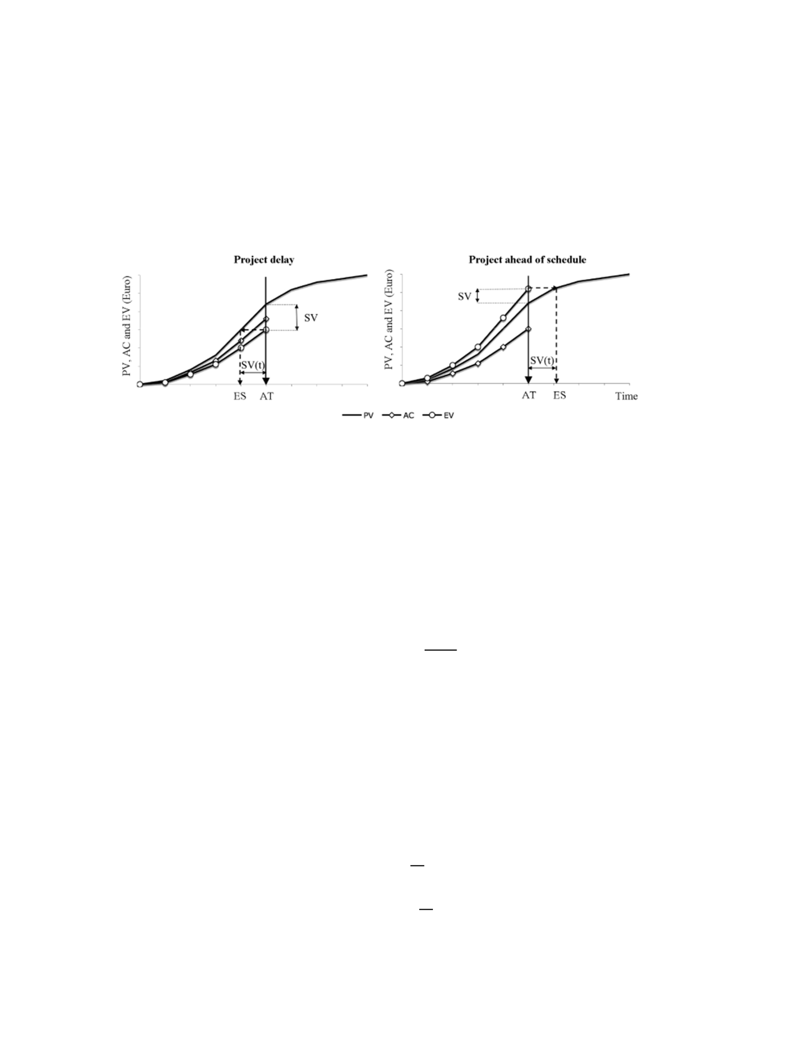
The graphical presentation above shows the difference between earned schedule when the

project is ahead of schedule as shown in the right and in case of the project is delayed as shown

in the figure on the left.

Where SV(t) is the schedule variance in time units and SV is schedule variance in cost units,

and AT is the actual time.

To calculate the Estimate at completion in time units the equation is as follows:

𝐸𝐴𝐶= 𝐴𝑇 + 



Equation 4 Estimate at Completion (Vanhoucke,2009)

Where AT is the actual time and PDWR is the planned duration for work remaining and PF is

the performance factor where PF = 1 when the duration of the remaining work is as planned

and PF = SPI(t) when the duration of remaining work is following the SPI(t) trend and PF =

SCI(t) when duration of remaining work is following the cost and time trend.

The calculation of SPI, SPI(t), SCI, SCI(t) is as follows:

SPI= 



SPI(t) = 



Figure 4: ES difference between two scenarios

Equation 5 Schedule Performance index (Vanhoucke,2009)

SCI = SPI X CPI

SCI(t) = SPI(t) X SCI

Equation 6 Schedule Cost Index (Vanhoucke,2009)

Finally, PDWR = PD – AT

Where PD is the planned duration and AT is the actual duration.

In order to examine the accuracy of the estimation the following equation is used:

Accuracy = | |



Equation 7 Accuracy (Vanhoucke,2009)

Where AD is the equal to the actual project finish date, and the EAC is the estimation at

completion.

2- Earned Duration Method uses the concept of earned duration and it is calculated using

the following formula:

ED Earned Duration = AD X SPI

Equation 8 Earned Duration (Vanhoucke,2009)

Where AD is the Actual duration and SPI is the schedule performance index and it is

calculated as before.

The Estimate at completion in time units using this method is called estimate duration at

completion (EDAC) and it is calculated as follows:

EDAC = AD + UDR

Equation 9 Estimate Duration at Completion (Vanhoucke,2009)

Where UDR is unearned duration remaining and AD is the actual duration.

UDR is calculated using the following formula where PD is the planned duration, ED is the

earned duration and PF is the performance factor.

UDR = 



Equation 10 Unearned Duration Remaining (Vanhoucke,2009)

Similar to the previous method performance factor could be PF = 1, SPI, SCI based on the

calculations of the remaining duration.

After that assess the accuracy of the estimation the following equation is used:

Accuracy = | |



Where EDAC is the estimate duration at completion and AD is the actual duration of the

project.

3- The third and final method is the planned value method which is calculated based on a

metric called planned value rate 𝑃𝑉

 and TV which the time variance.

𝑃𝑉

= 𝐵𝐴𝐶

𝑃𝐷

Equation 11 Planned Value rate (Vanhoucke,2009)

𝑃𝑉

 is the planned rate per time to finish the project on time where BAC = budget at completion

and PD is the planned project duration.

As for the time variance (TV) is the difference in time between the planned budget and actual

cost in time units and it is calculated using the following equation:

𝑇𝑉 = 𝑆𝑉

𝑃𝑉



Equation 12 Time Variance (Vanhoucke,2009)

Where SV is the schedule variance, and it is calculated as follows SV = EV – PV

With the 𝑃𝑉

 the time variance is calculated.

The calculation of the estimate at completion is calculated using TEAC which is time estimate

at completion and it is calculated using this formula TEAC = PD – TV when the remaining

work is following the plan, when the remaining work is following the SPI trend, this formula

is used

𝑇𝐸𝐴𝐶 = 𝑃𝐷

𝑆𝑃𝐼

Equation 13 Time Estimate At Completion (Vanhoucke,2009)

Finally, when the remaining work is following the SCI trend the following formula is used.

𝑇𝐸𝐴𝐶 = 𝑃𝐷

𝑆𝐶𝐼

Similarly, the accuracy is of the estimation is calculated using the following equation:

Accuracy = ||



3.8. Ethical Considerations

To maintain confidentiality and ethical standards, the names of the contractors and specific

project details were excluded from this research. Instead, projects were categorized by type,

such as commercial, educational, power stations, renovation, administrative, and residential.

Chapter 4: Data Collection

In this chapter, we provide an overview of the data collection process for the analysis of 30

construction projects across various cities in Egypt. These projects were selected from different

sectors, including commercial, educational, power stations, renovation, administrative, and

residential projects. The data collection process involved a combination of methods, tools, and

sources to gather relevant information for our analysis.

4.6 Projects Overview

The outcomes derived from site visits and interviews include the collection of BCWP, ACWP,

and BCWS data from 30 projects.

1. Budgeted Cost of Work Performed (BCWP): BCWP, also known as EV, represents the

value of the work that has actually been completed in monetary terms. This metric reflects

the progress made in a project and is measured on a monthly basis to track how much of

the planned work has been accomplished.

2. Budgeted Cost of Work Scheduled (BCWS): BCWS, also referred to as PV, signifies the

budgeted value of the work that was originally scheduled to be completed during a specific

period. It provides a planned baseline for project performance and is assessed monthly to

compare the planned progress with the actual progress.

3. Actual Cost of Work Performed (ACWP): ACWP represents the actual costs incurred

during a given month in executing the project. This metric is essential for monitoring

project expenses and determining the financial aspects of project execution.

Additionally, both the original schedules and actual schedules were gathered to facilitate

the analysis of the collected data. The detailed presentation of the data collected for each project

will be provided below. The projects used will be discussed in briefly in the table below and in

details.

Table 2 Projects Data collected.

T BCWS

(EGP)

BCWP

(EGP)

ACWP

(EGP)

(D )

1 160,387,330 160,387,330 171,886,590 -11,499,260 20-Feb-18 30-Oct-18 -252

2 E 145,263,973 145,263,973 157,985,453 -12,721,480 30-Apr-17 20-Dec-17 -234

3 I 322,179,850 322,179,850 334,650,146 -12,470,296 19-Apr-19 30-Sep-19 -164

Project 1: Commercial Project

Project 1 commenced on March 1, 2015, with a planned completion date of February 20, 2018.

However, it encountered delays, resulting in an actual finish date of October 30, 2018, which

was 252 days behind schedule. The project had a planned budget of 160 million EGP, but the

actual cost amounted to 172 million EGP, exceeding the budget by 12 million EGP. The

Schedule Performance Index (SPI) started at 76% but dropped to 55%, indicating that the

project was both over budget and behind schedule.

Project 2: Educational Project

This educational project began on July 25, 2015, with a scheduled completion date of April 30,

2017. Unfortunately, it faced delays and ultimately finished on December 20, 2017, 234 days

later than planned. The planned budget was 145 million EGP, but the actual cost reached 157

million EGP, resulting in a 12 million EGP budget overrun. The SPI started at 92% but declined

to 66%, indicating that the project was both over budget and behind schedule.

4 498,371,317 498,371,317 510,650,568 -12,279,251 4-Sep-19 30-Nov-20 -453

5 R 1,844,515,667 1,328,283,068 1,297,649,614 30,633,454 13-Jan-23 30-Jun-23 -169

6 505,782,177 505,782,177 455,858,281 49,923,896 30-Mar-21 30-May-21 -61

7 R 129,946,203 129,946,203 149,674,697 -19,728,494 30-Sep-21 30-Dec-21 -91

8 E 524,011,456 524,011,456 491,657,287 32,354,169 25-Sep-20 20-Nov-20 -56

9 R 934,084,850 869,551,166 908,852,210 -39,301,044 25-Oct-21 28-Feb-23 -491

10 101,460,922 101,460,922 103,647,402 -2,186,480 20-Mar-16 28-Feb-17 -345

11 278,072,672 278,072,672 276,227,816 1,844,856 7-Dec-21 30-Nov-22 -358

12 224,382,775 224,382,775 231,577,203 -7,194,428 1-Oct-19 31-Mar-20 -182

13 I 391,381,394 391,381,394 345,945,404 45,435,990 21-Feb-17 30-Dec-17 -312

14 E 237,039,879 237,039,879 228,301,480 8,738,399 20-Jul-19 14-Sep-19 -56

15 106,717,901 106,717,901 99,209,499 7,508,402 31-Dec-20 25-Jan-21 -25

16 209,859,079 209,859,079 237,328,844 -27,469,765 17-Nov-22 30-Jun-23 -225

17 E 583,273,944 583,273,944 677,666,732 -94,392,788 17-Apr-23 30-Oct-23 -196

18 550,151,073 489,264,996 553,748,233 -64,483,237 4-Aug-22 30-Mar-23 -239

19 I 154,528,736 154,528,736 136,354,130 18,174,606 20-Jun-20 29-Jul-21 -404

20 758,418,631 758,418,631 628,632,758 129,785,873

31-May-22 30-Mar-23 -303

21 R 39,050,912 39,050,912 38,163,075 887,837 22-Apr-20 30-Jun-20 -69

22 I 1,540,046,857 1,540,046,857 1,253,676,323 286,370,534

12-May-20 30-Sep-21 -506

23 I 188,803,564 188,803,564 200,787,624 -11,984,060 3-Apr-21 15-Jun-21 -73

24 61,742,362 61,742,362 57,837,539 3,904,823 30-Jan-19 30-Apr-19 -90

25 341,780,342 341,780,342 360,220,926 -18,440,584 23-Jan-23 30-Dec-23 -341

26 74,027,664 74,027,664 80,492,656 -6,464,992 26-May-22 30-Aug-23 -460

27 172,742,103 172,742,103 192,355,326 -19,613,223 2-Mar-20 30-Dec-20 -303

28 R 299,554,952 299,554,952 339,899,961 -40,345,009 24-Jul-17 30-Apr-18 -280

29 I 167,766,090 167,766,090 160,622,767 7,143,323 31-Jan-19 30-Apr-19 -89

30 I 106,927,735 106,927,735 95,321,477 11,606,258 15-Feb-17 30-Sep-17 -227

Project 3: Power Station Project

Project 3 was a power station project that was initially planned to start on November 5, 2017,

and finish on April 19, 2019. However, it experienced delays and concluded on September 30,

2019, 164 days later than scheduled. The planned budget for the project was 322 million EGP,

but the actual cost amounted to 335 million EGP, resulting in a 13 million EGP budget

deviation. The SPI trend began at around 50% and improved to 87%, with an average SPI of

approximately 80%. Nevertheless, the project was both over budget and behind schedule.

Project 4: Commercial Project

Project 4, a commercial project, was initiated on May 6, 2017, with a planned completion date

of September 4, 2019. However, it faced scheduling challenges, resulting in an actual finish

date of November 30, 2020, which was 453 days later than anticipated. The project was

budgeted at 498 million EGP, and the actual cost reached 510 million EGP, exceeding the

budget by 12 million EGP. The SPI trend showed fluctuations, starting on schedule, and

dropping to 43%, and the CPI trend fluctuated between 88% and 95%. Consequently, the

project was both over budget and behind schedule.

Project 5: Residential Project

This residential project was set to commence on January 14, 2021, with a planned finish date

of January 13, 2023. Unfortunately, it experienced delays, and the forecasted finish date

extended to March 31, 2023, resulting in a deviation of 78 days from the original schedule. The

SPI trend began at 117% but dropped to 76%, indicating that the project was behind schedule.

On the other hand, the CPI trend remained nearly constant at 105%, indicating that the project

was under budget.

Project 6: Commercial Project

Project 6, another commercial project, was scheduled to begin on September 29, 2019, and

conclude on March 30, 2021. However, it faced setbacks, and the actual finish occurred on

May 30, 2021, with a 61-day deviation from the original plan. The planned budget for the

project was 505 million EGP, but the actual cost was 455 million EGP, resulting in a budget

surplus of nearly 50 million EGP. The CPI trend remained consistently at 111%, indicating that

the project was under budget, although it was behind schedule.

Project 7: Renovation Project

A renovation project, Project 7, was slated to start on March 10, 2018, and finish on September

30, 2021. However, it experienced delays and was completed on December 30, 2021, with a

91-day deviation from the planned schedule. The planned budget for the project was 130

million EGP, but the actual cost reached 150 million EGP, resulting in a 20 million EGP budget

overrun. The SPI trend started at 110% but decreased to 97%, and the CPI began at 130% and

decreased to 87%. Consequently, the project was both over budget and behind schedule.

Project 8: Educational Project

Project 8, an educational project, was set to commence on September 25, 2019, and conclude

on September 25, 2020. However, it faced scheduling challenges and was completed on

November 20, 2020, 56 days later than planned. The planned budget for the project was 524

million EGP, while the actual cost was 492 million EGP, resulting in an underspend of 32

million EGP. The SPI trend started at 95% but fluctuated, while the CPI trend showed an

average of 108%. Consequently, the project was under budget but behind schedule.

Project 9: Commercial Project

Project 9, also a commercial project, was planned to start on October 19, 2014, and finish on

March 20, 2016. However, it experienced a significant drop in the SPI, reaching around 55%,

and concluded on February 28, 2017, with an extra 345 days compared to the planned schedule.

The planned budget was 101 million EGP, and the actual cost amounted to 103 million EGP,

resulting in a 2 million EGP budget deviation. The CPI remained at around 96% throughout

the project, indicating that the project was both behind schedule and over budget by 2 million

EGP.

Project 10: Residential Project

Project 10, a residential project, was planned to start on September 28, 2020, and finish on

October 25, 2021, with a total duration of 757 days. However, the SPI trend started at 85% and

declined to 62%, and the project was forecasted to finish on February 28, 2023, with a deviation

of 491 days from the original schedule. The planned budget was 934 million EGP, and the

actual cost was 908 million EGP, resulting in an overspend of 26. The CPI trend started at

111% and dropped to 96%. Consequently, the project was behind schedule and over budget.

Project 11: Administrative Project

Project 11, an administrative project, was scheduled to start on December 8, 2020, and finish

on December 7, 2021, with an overall duration of 364 days. However, the SPI trend started at

90% and dropped to 35%, resulting in the project finishing on November 30, 2022, with a

deviation of 358 days from the original plan. The CPI trend began at 133% and decreased to

98%. Based on the CPI percentage, the project budget was 278 million EGP, and the actual

cost was 276 million EGP, indicating that the project was under budget by 2 million EGP.

Project 12: Commercial Project

Project 12, another commercial project, was planned to start on May 10, 2018, and end on

October 1, 2019. Unfortunately, it faced scheduling issues as the SPI dropped to 70%, resulting

in the project concluding on March 31, 2020, with a deviation of 182 days from the schedule.

The planned budget was 224 million EGP, and the actual cost was 231 million EGP, resulting

in a budget deviation of 7 million EGP. The CPI trend fluctuated between 108% and 101%.

Consequently, the project was behind schedule but within budget.

Project 13: Industrial Project

Project 13, an industrial project, was scheduled to start on December 1, 2015, and finish on

February 21, 2017. However, the SPI dropped to 75%, leading to the project's completion on

December 30, 2017, with a deviation of 312 days from the planned schedule. The project

budget was not disclosed, but the cost performance index ranged from 102% to 114%, and the

project concluded with a CPI of 113%. This indicated that the project was under budget but

behind schedule.

Project 14: Educational Project

Project 14, an educational project, was planned to start on September 9, 2018, and end on July

20, 2019, with an initial duration of 314 days. However, the SPI dropped from 96% to 75%,

resulting in the project's completion on September 14, 2019, with a deviation of 56 days. The

cost performance index (CPI) began at 111% but dropped to 104%, indicating that the project

was under budget but behind schedule.

Project 15: Commercial Project

Project 15 was a commercial project set to start on October 13, 2019, and finish on December

31, 2020. However, the SPI fluctuated between 105% and 95%, causing the project to be

completed on January 25, 2021, with a 25-day delay. The planned budget for the project was

not disclosed, but the CPI ranged from 127% to 108%, ending at 108%. The project was behind

schedule but within budget.

Project 16: Commercial Project

Project 16, another commercial project, was planned to start on November 17, 2021, and end

on November 17, 2022. However, the SPI dropped from 90% to 69%, resulting in the project's

completion on June 30, 2023, with a deviation of 225 days. The planned budget for the project

was not disclosed, but the CPI trend started at 111% and dropped to 88%. The project was both

over budget and behind schedule.

Project 17: Commercial Project

Project 17, a commercial project, was scheduled to start on April 20, 2021, and finish on April

17, 2023. However, the SPI trend started at 105% and dropped to 72%, resulting in a

completion date of October 30, 2023, with a 196-day deviation from the planned schedule. The

planned budget for the project was 583 million EGP, but the actual cost reached 677 million

EGP, resulting in a 94 million EGP budget overrun. The SPI trend indicated that the project

was both over budget and behind schedule.

Project 18: Commercial Project

Project 18 was a commercial project planned to start on December 15, 2021, and finish on

August 4, 2022. The expected actual finish date was March 30, 2023, with a deviation of 239

days. The planned budget for the project was 550 million EGP, the earned value was 489

million EGP, and the actual cost was 553 million EGP, indicating a budget deficit of 64 million

EGP. The SPI was 80%, and the CPI was 88%, demonstrating that the project was behind

schedule and over budget.

Project 19: Industrial Project

Project 19, an industrial project, was intended to start on December 20, 2018, and finish on

June 20, 2020. However, it concluded on July 29, 2021, with a deviation of 89 days. The

planned budget was 154 million EGP, and the actual cost was 136 million EGP, resulting in an

underspend of 18 million EGP. The SPI was 49%, and the CPI was 113%, indicating that the

project was behind schedule but under budget.

Project 20: Commercial Project

Project 20, another commercial project, was planned to start on January 22, 2020, and finish

on May 31, 2022. However, the project was completed on March 30, 2023, with a 303-day

delay. The planned budget was 758 million EGP, and the actual cost was 628 million EGP,

resulting in an underspend of 130 million EGP. The SPI was 68%, and the CPI was 121%,

demonstrating that the project was behind schedule but under budget.

Project 21: Residential Project

This residential project was scheduled to begin on August 22, 2019, and finish in 2020, but it

concluded on June 30, 2020, with a 69-day deviation. No cost deviation information was

provided.

Project 22: Industrial Project

Project 22 was an industrial project that was planned to start on November 12, 2018, and finish

on May 12, 2020. However, it finished on September 30, 2021, with a deviation of 506 days

from the planned duration. The planned budget was 1540 million EGP, but the actual cost was

1253 million EGP, indicating a budget deviation of 286 million EGP. The SPI was 66%, and

the CPI was 123%, showing that the project was behind schedule and under budget.

Project 23: Industrial Project

Project 23 was an industrial project that was planned to start on May 3, 2020, and finish on

April 3, 2021. However, it finished on June 15, 2021, with a delay of 73 days from the planned

duration. The planned budget was 189 million EGP, but the actual cost was 201 million EGP,

indicating a budget deviation of 12 million EGP. The SPI was 94%, and the CPI was 73%,

showing that the project was behind schedule and over budget.

Certainly, here's a rephrased version of the information about Projects 24 to 30 in paragraph

format:

Project 24: Commercial Project

Project 24 falls under the category of commercial projects. Originally scheduled to commence

on June 1, 2018, and conclude by January 30, 2019, it faced a deviation, finishing on April 30,

2019, marking a 90-day delay. The Schedule Performance Index (SPI) at the planned duration

was 54%. In terms of budget, it's important to note that the project consistently remained under

budget throughout its duration, concluding with an actual cost of 58 million EGP compared to

the planned budget of 62 million EGP, resulting in a 4 million EGP budget surplus.

Project 25: Commercial Project

Project 25 is another commercial project that was initially planned to kick off on August 15,

2021, and wrap up by January 23, 2023. Unfortunately, due to low performance, it concluded

on December 30, 2023, reflecting a significant deviation of 341 days from the original plan,

which was a 526-day schedule. The SPI at the planned duration was at 61%. In terms of costs,

the Cost Performance Index (CPI) began under budget at 111% but progressively decreased to

95% by the project's end, resulting in a 19 million EGP deviation from the planned budget of

342 million EGP, with an actual cost of 360 million EGP.

Project 26: Commercial Project

Project 26, also classified as a commercial project, was initially intended to start on May 18,

2021, and conclude on May 26, 2022. However, it faced substantial delays, concluding on

August 30, 2023, resulting in a total duration of 834 days instead of the planned 373 days. The

SPI at the planned duration was 65%. On the cost front, the project initially operated under

budget, but it gradually moved into an over-budget scenario, with a final CPI of 92%.

Project 27: Commercial Project

Project 27, another commercial project, was initially scheduled to begin on October 1, 2019,

and end on March 2, 2020. However, the project faced significant delays, concluding on

December 30, 2020, representing a total deviation of 303 days from the planned duration,

which was initially set at 153 days. The SPI at the end of the project was 56%. In terms of

costs, the project experienced a continuous state of being over budget, with a CPI of 95% at

the start and 90% at the conclusion.

Project 28: Residential Project

Project 28 falls into the residential project category. It was planned to start on March 23, 2015,

and finish by July 24, 2017. However, the project experienced a substantial delay, concluding

on April 30, 2018, marking a total deviation of 280 days from the planned 854-day duration.

The project consistently lagged behind schedule. On the cost side, it was over budget

throughout its duration, with a 40 million EGP deviation from the planned budget of 300

million EGP, concluding with an actual cost of 340 million EGP.

Project 29: Industrial Project

Project 29 is an industrial project that was initially scheduled to begin on July 2, 2018, and

conclude by December 31, 2019. However, the project finished on April 30, 2019, with an 89-

day deviation from the planned duration, primarily due to low performance and a low SPI.

From a cost perspective, the project remained under budget throughout, with a 7 million EGP

budget surplus when compared to the planned budget of 167 million EGP and an actual cost of

160 million EGP.

Project 30: Industrial Project

Finally, Project 30, another industrial project, was planned to begin on June 5, 2016, and

conclude by February 15, 2017, representing a total duration of 255 days. However, the project

faced extensive delays, concluding on September 30, 2017, with an actual duration of 482 days,

resulting in a 227-day deviation from the planned finish date. The project was behind schedule

primarily due to low performance, with an SPI of 50% at the planned finish date. In terms of

costs, the project consistently remained under budget, concluding with an actual cost of 95

million EGP compared to the planned budget of 107 million EGP, resulting in an 11 million

EGP budget surplus.

4.7 Conclusion

In this Chapter, the data collection process, and an overview of the 30 projects analyzed for

this study. The projects were collected from various cities across Egypt, including Cairo, Ain

Sokhna, Alexandria, North Coast, Gouna, Giza, and 6th of October. These projects encompass

a diverse range of types, including residential, commercial, administrative, renovation,

educational, and power station construction. Subset of these projects were examined in detail

to highlight the data collection process and provide insights into their schedules and budgets.

In the following chapter (Chapter 5), we will delve into the data analysis techniques that will

be applied to this dataset. These techniques include the earned schedule method, earned

duration method, and planned value method, each of which will be discussed in detail to

provide a comprehensive understanding of the project performance metrics and trends.

Chapter 5: Analysis

In this chapter, We compare the three methods of EVM which are earned schedule method,

earned duration method, and planned value method on 30 actual projects in order to find an

accurate estimation of the finish date and define which method fits best in different cases. The

projects have different types such as commercial, industrial, educational, residential,

renovation and administrative. These projects are located in different cities across Egypt such

as Cairo, Giza, 6th of October, Ain Sokhna, Hurghada, North coast and Alexandria. These

projects have different timelines ranging from 2015 to 2023, in addition to different contract

prices. All these projects were evaluated from the contractor’s point of view. The projects data

were collected from various contractors across Egypt.

5.1 Demonstrating Calculation Procedures in the Sample Project

The calculations will be remonstrated in one project in order to show how the

calculations works, the project used for these calculations is a commercial project with a total

budget of 498 million EGP the project started in 06th May 2017 and it was planned to finish on

4th September 2019 and actual finish is 30th November 2020. The Month that will be using the

calculations for is 01st November 2018 in which the earned value is 127,800,365 million EGP

while the actual cost is 145,807,922 and the planned value is 255,378,951 million EGP.

The analysis incorporated three distinct earned value techniques: Earned Duration method,

Earned Schedule method, and Planned Value method. Each method had its own set of metrics

to evaluate project performance and forecasting accuracy of calculating finish date:

1- Earned Duration Method:

Earned Duration (ED): This metric indicates the equivalent duration based on the value

of work completed. It quantifies the time required to complete the earned value.

In a related context, Jacob and Kane (2004) introduced a concept, earned duration (ED),

which is the result of multiplying the actual project duration (AD) by the schedule

performance index (SPI). Jacob (2003) and Jacob and Kane (2004) advocated for the earned

duration method as a robust approach for forecasting a project's final duration by

incorporating the schedule performance index (SPI).

The earned duration is calculated using the following formula.

ED Earned Duration = AD X SPI

The actual duration AD is 544 days and the SPI = 

 = ,,

,, = 50%

Then the Earned duration is calculated ED = 50% x 544 = 272 Days

After that estimate at completion is calculated using this formula EDAC = 𝐴𝐶 + 



PD is the planned total duration of the project which is 851 days and earned duration is 272

days.

The estimate at completion will be calculated three times, the first time when the performance

factor PF = 1, the second time when the PF is equal to SPI, and the third time when the PF is

equal to SCI which schedule cost index.

𝐸𝐴𝐶=544 + 

 = 1123 Days

At PF = SPI

𝐸𝐴𝐶=544 + 

. = 1702 Days

At PF = SCI

SCI = SPI x CPI

CPI = = 

 = ,,

,, = 88%

SCI = SPI x CPI = 88% x 50% = 44%

𝐸𝐴𝐶=544 + 

. = 1865 Days

The actual finish date 30th November 2020 and the actual project duration is 1304 days.

Then the three estimates are compared with the actual finish date and the accuracy is calculated

𝐴𝑐𝑐𝑢𝑟𝑎𝑐𝑦 = 1 − ||

 = = ||

 = 86%

𝐴𝑐𝑐𝑢𝑟𝑎𝑐𝑦 = 1 − ||

 = = ||

 = 69%

𝐴𝑐𝑐𝑢𝑟𝑎𝑐𝑦 = 1 − ||

 = = ||

 = 57%

Therefore, the highest accuracy achieved when the PF = 1

2- Planned Value Method:

Anbari (2003) developed the planned value method, which relies on established earned

value metrics to project a project's duration. This method calculates the average planned

value per time period, known as the planned value rate (PVrate). PVrate is determined by

dividing the project's baseline budget at completion (BAC) by its planned duration (PD).

This metric helps translate schedule variance (SV) into time units, represented as time

variance (TV).

First planned value rate is calculated as shown below:

𝑃𝑉

= 

 = ,,

 = 585,630

Then time variance is calculated.

𝑇𝑉 = 𝑆𝑉

𝑃𝑉



SV = EV – PV = 127,800,365 - 255,378,951 = -127,579,585 EGP

𝑇𝑉 =  ,,

, = -218 days

After that estimate at completion is calculated when the performance factor = 1 using this

formula

𝑇𝐸𝐴𝐶= PD – TV = 851 – (-218) = 1069 days

At PF = SPI

Time variance is calculated using this formula 𝑇𝐸𝐴𝐶 = 

 = 

% = 1702 days

At PF = SCI

The time variance is calculated using this formula 𝑇𝐸𝐴𝐶 = 

 = 

% = 1942 days

Then the three estimates are compared with the actual finish date and the accuracy is calculated

𝐴𝑐𝑐𝑢𝑟𝑎𝑐𝑦 = 1 − ||

 = = ||

 = 82%

𝐴𝑐𝑐𝑢𝑟𝑎𝑐𝑦 = 1 − ||

 = = ||

 = 69%

𝐴𝑐𝑐𝑢𝑟𝑎𝑐𝑦 = 1 − | |

 = = ||

 = 51%

Therefore, the highest accuracy achieved with planned value method is when PF = 1

3- Earned Schedule Method:

Earned Schedule (ES): ES represents the time when the value of the work is earned. It is

calculated using the following formula:

𝐸𝑆 = t +  





 = 544 + ,, ,,

,,,, = 330 Day

To calculate the Estimate at completion in time units the equation is as follows:

First at PF = 1,

𝐸𝐴𝐶 = 𝐴𝑇 + 

 = 𝐴𝑇 + 

 = 544 + 

 = 1065 day

at PF = SPI,

𝐸𝐴𝐶 = 𝐴𝑇 + 

 = 𝐴𝑇 + 

 = 544 + 

% = 1403 day

at PF = SCI,

𝐸𝐴𝐶 = 𝐴𝑇 + 

 = 𝐴𝑇 + 

 = 544 + 

% = 1524 day

Comparing the result with the actual finish date, the accuracy is determined as shown below.

𝐴𝑐𝑐𝑢𝑟𝑎𝑐𝑦 = 1 − ||

 = = ||

 = 82%

𝐴𝑐𝑐𝑢𝑟𝑎𝑐𝑦 = 1 − | |

 = = ||

 = 92.4%

𝐴𝑐𝑐𝑢𝑟𝑎𝑐𝑦 = 1 − ||

 = = | |

 = 83%

Therefore, the highest accuracy achieved with earned schedule is when PF = SPI, in addition

to being the highest accuracy obtained

Following the project calculations, the results will be presented in four figures. These

figures will depict the project duration percentages under different scenarios: first, when the

performance factor is set to 1; second, when the performance factor is configured to SPI; third,

when the performance factor is set to SCI; and finally, a comprehensive comparison figure to

assess the overall estimation. This comparison will highlight the most suitable technique to

employ based on the performance factor.

figure 6 presents an average comparison among the three techniques for the

demonstrative project. As depicted, the Earned Schedule method demonstrates consistent

accuracy between 75% and 90% throughout the project duration. In contrast, the Earned

Duration method exhibits a decline from 20% to 75% of the project duration, followed by a

subsequent increase leading to its peak accuracy at the conclusion of the project. Likewise, the

Planned Value method experiences a decrease from 20% to 75% of the project duration,

reaching its lowest accuracy among the three techniques by the project's end.

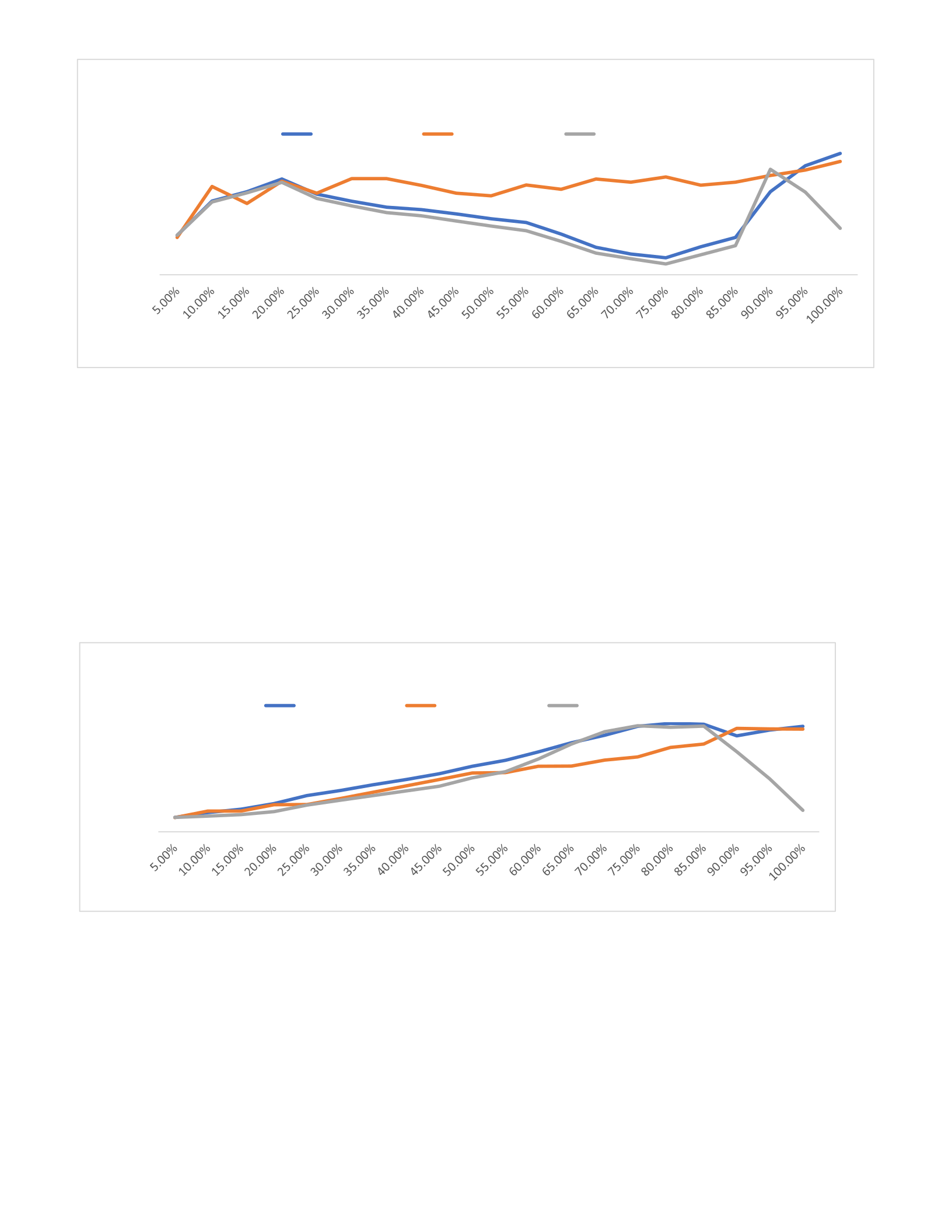
Figure 7 offers a comparative assessment of the three techniques when the performance

factor is equal to 1. Initially, all three methods exhibited nearly identical accuracy, hovering

around 65%. Subsequently, as the project duration percentage advanced to 85%, all methods

showed a continuous increase. However, a notable divergence occurred thereafter: the Planned

Value method began to decline, reaching approximately 69% towards the project's conclusion.

In contrast, the Earned Schedule method achieved a 97.5% accuracy by the project's end, while

the Earned Duration method reached the highest percentage, standing at 98.5% at the

conclusion of the project.

Figure 8 provides a comparative evaluation of the three techniques when the

performance factor is set to SPI. Initially, all three methods demonstrated nearly identical

accuracy, hovering around 65%. As the project duration percentage advanced to 20%, all three

methods experienced an increase. However, a divergence emerged after this point: the Planned

Duration and Earned Duration methods gradually decreased, reaching their lowest points

around the 75% duration mark. In contrast, the Earned Schedule method-maintained accuracy

50%

55%

60%

65%

70%

75%

80%

85%

90%

95%

100%

Accuracy

Duration Percentage

AVER AGE E ARN ED S CHEDULE VS E ARNE D DUR ATION VS

PLANN ED DUR ATION

Earned Duration Earned Schedule Planned Value

60%

65%

70%

75%

80%

85%

90%

95%

100%

Accuracy

Duration Percentage

EARNED SC HEDULE VS EARNED DUR ATIO N VS P LANNED

DURATION AT PF =1

Earned Duration Earned Schedule Planned Value

Figure 7 Average accuracy Earned schedule vs earned duration vs planned duration At PF = 1

Figure 6 Average Earned Schedule VS earned Duration VS Planned Duration

between 85% and 95% throughout the project duration, concluding with a 94% accuracy.

Towards the end of the project, the Earned Duration method exhibited an increase, reaching

98%, while the Planned Value method declined, concluding with a 68% accuracy.

Figure 9 conducts a comparative assessment of the three techniques with the

performance factor set to SCI. Initially, all three methods demonstrated virtually identical

accuracy, hovering around 65%. As the project duration percentage progressed to 20%, two

methods, namely Earned Schedule and Planned Value, exhibited an increase, maintaining

accuracy between 80% and 95% throughout the project duration and culminating in a 94%

accuracy by the project's conclusion. In contrast, Earned Duration experienced a decline,

reaching 29% at the 75% mark of the project duration percentage. Subsequently, it underwent

an upward trend, reaching 98% by the conclusion of the project.

40%

45%

50%

55%

60%

65%

70%

75%

80%

85%

90%

95%

100%

Accuracy

Duration Percentage

EARNED SCHEDULE VS EARNED DURATION VS

PLANNED DURATION AT PF =SPI

Earned Duration Earned Schedule Planned Value

25%

30%

35%

40%

45%

50%

55%

60%

65%

70%

75%

80%

85%

90%

95%

100%

Accuracy

Duration Percentage

EARNED SCHEDULE VS EARNED DURATION VS PLANNED

DURATION AT PF =SCI

Earned Duration Earned Schedule Planned Value

Figure 8 Average accuracy Earned schedule vs earned duration vs planned duration At PF = SPI

Figure 9 Average accuracy Earned schedule vs earned duration vs planned duration At PF = SCI

 However, it's worth noting that the choice of the most effective technique also depends on

the specific project type and its duration. For renovation and residential projects, the Earned

Schedule method outperformed the others, achieving the highest accuracy. On the other

hand, for industrial, commercial, and educational, the Earned Duration method was

consistently the most accurate.

5.2 The Analysis of Industrial Projects.

The detailed discussion of the outcomes for each project type begins with industrial projects.

As previously noted, the Earned Duration method yields the highest overall percentage.

However, when the performance factor is set to SPI, Earned Schedule takes the lead in

accuracy. The following illustration provides a comprehensive overview of accuracy

percentages across project duration percentages, considering performance factors 1, SPI, SCI,

and the average.

Figure 10 depicts the accuracy comparison among the three methods on an average basis.

Figure 11 illustrates the comparison of accuracy among the three methods under the condition

of a performance factor set to 1.

55%

60%

65%

70%

75%

80%

85%

90%

95%

100%

Accuracy

Duration Percentage

AVER AGE COMPARIS ON BE TWE EN EA RNED S CHEDULE VS

EAR NED DU RATION VS P LANNED DURATION ( INDUS TR IAL

PR OJ ECTS )

Earned Duration Earned Schedule Planned Value

60%

65%

70%

75%

80%

85%

90%

95%

100%

Accuracy

Duration Percentage

EARNED SC HE DULE VS EARNED DUR ATION VS PLA NNED

DURATION AT PF = 1 (IN DUST RIAL PRO J ECTS )

Earned Duration Earned Schedule Planned Value

Figure 10 Average Accuracy between Earned Schedule vs Earned duration vs Planned duration (Industrial Projects)

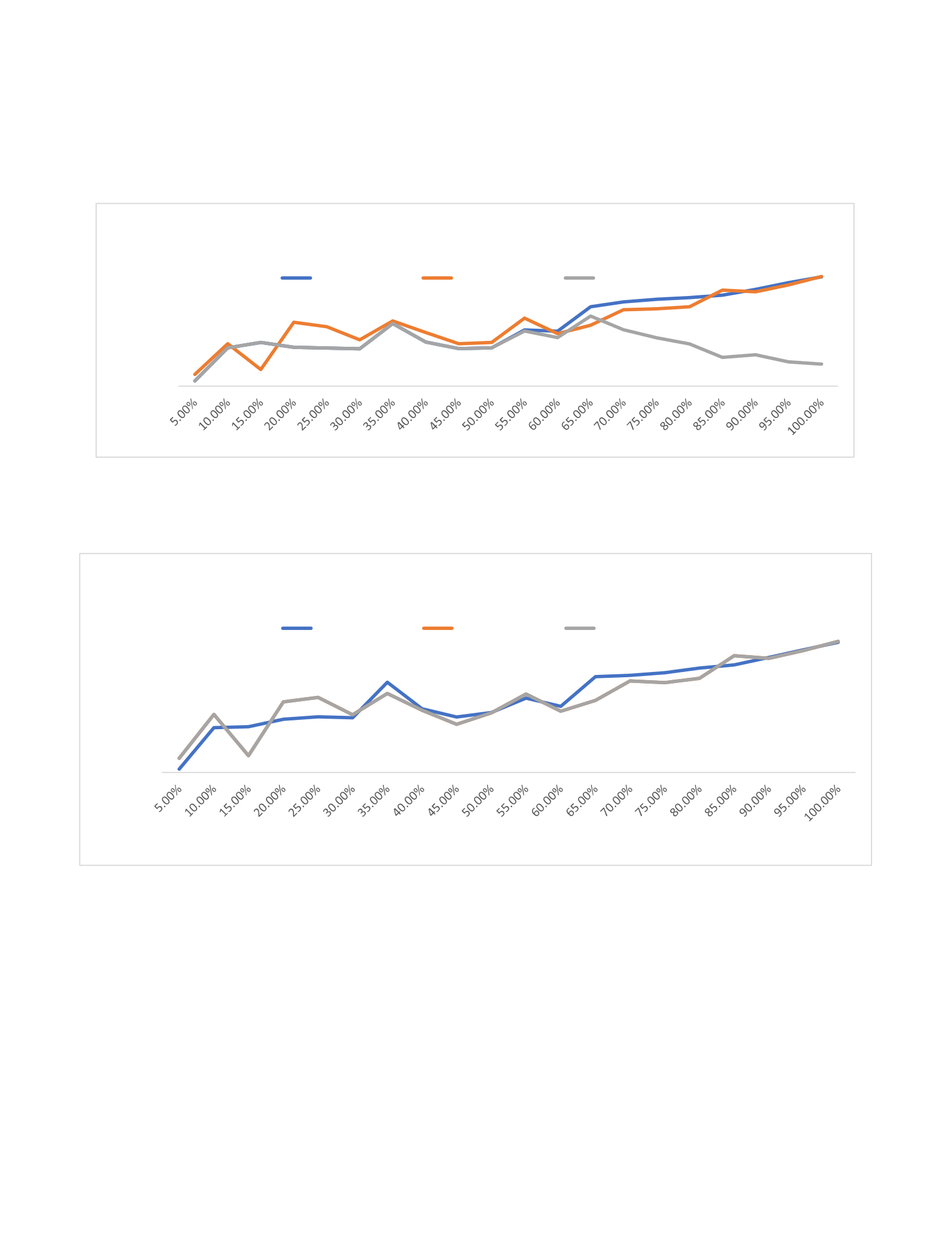
Figure 12 displays the accuracy comparison among the three methods when the performance

factor is set to SPI.

The fourth and final visual representation for the industrial project showcases the accuracy

comparison under the condition of a performance factor set to SCI.

Figure 13 displays the accuracy comparison among the three methods when the performance

factor is set to SCI.

5.3 The Analysis of Commercial Projects.

Similarly, in commercial projects, the Earned Duration method attains the highest

overall percentage, and this trend persists when the performance factor is set to 1. Conversely,

when the performance factor is SPI, the highest accuracy percentage is achieved by the Earned

Schedule method. The forthcoming illustration will present a comprehensive overview of

accuracy percentages across project duration percentages for performance factors 1, SPI, SCI,

and the average.

55%

60%

65%

70%

75%

80%

85%

90%

95%

100%

Accuracy

Duration Percentage

EARNED SC HE DULE VS EARNED DUR ATION VS PLA NNED

DURATION AT P F = SPI (IN DU STR IA L PROJ ECTS)

Earned Duration Earned Schedule Planned Value

50%

55%

60%

65%

70%

75%

80%

85%

90%

95%

100%

Accuracy

Duration Percentage

EAR NED S C HEDULE VS EARN ED DUR ATIO N VS PLANNE D

DURATION AT P F = SCI (INDU S TR IA L PROJ EC TS )

Earned Duration Earned Schedule Planned Value

Figure 11 Accuracy comparison between Earned Schedule vs Earned duration vs Planned duration (Industrial Projects) AT PF = 1

Figure

12 Average comparison between Earned Schedule vs Earned duration vs Planned duration (Industrial Projects) AT PF =SPI

Figure 13 Average comparison between Earned Schedule vs Earned duration vs Planned duration (Industrial Projects) at PF = SI

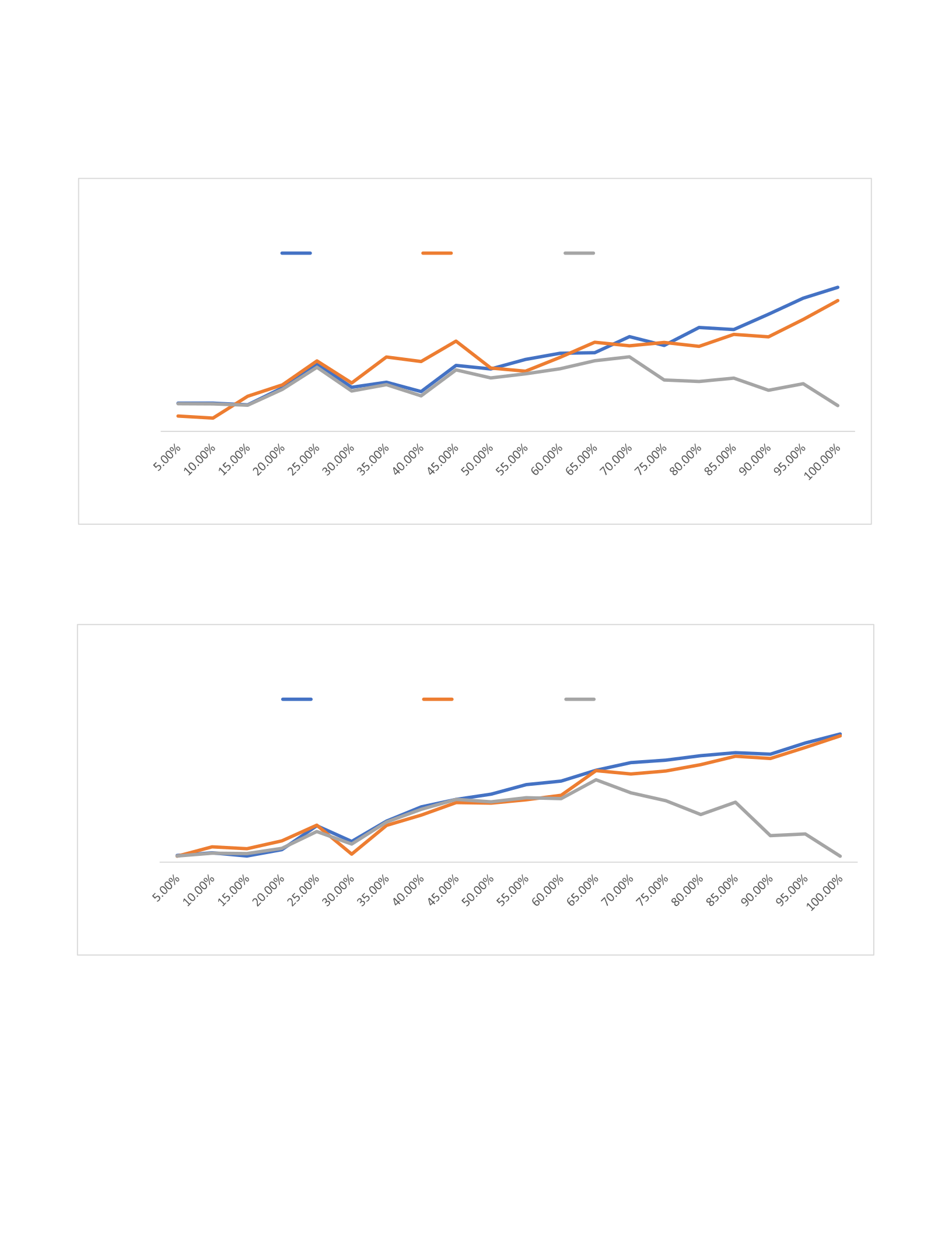
Figure 14 illustrates the comparison of accuracy among the three methods on an average scale.

Figure 15 depicts the accuracy comparison among the three methods when the

performance factor is set to 1.

Figure 16 showcases the accuracy comparison among the three methods when the performance

factor is configured to SPI.

65%

70%

75%

80%

85%

90%

95%

100%

Accuracy

Duration Percentage

EAR NED S CHEDULE VS EAR NED DUR ATIO N VS PLANNE D

DURATION AT PF =1 ( COMMET RIAL PROJ EC TS)

Earned Duration Earned Schedule Planned Value

Figure 14 Average Earned Schedule vs Earned duration vs Planned duration (Commetrial Projects)

Figure

Average Earned Schedule vs Earned duration vs Planned duration (Commetrial Projects)

at PF = 1

60%

65%

70%

75%

80%

85%

90%

95%

100%

Accuracy

Duration Percentage

AVER AGE EA RNED S CHEDULE VS EAR NE D DUR ATION VS

PLAN NED DUR ATION (C OM MET RIAL PROJ EC TS)

Earned Duration Earned Schedule Planned Value

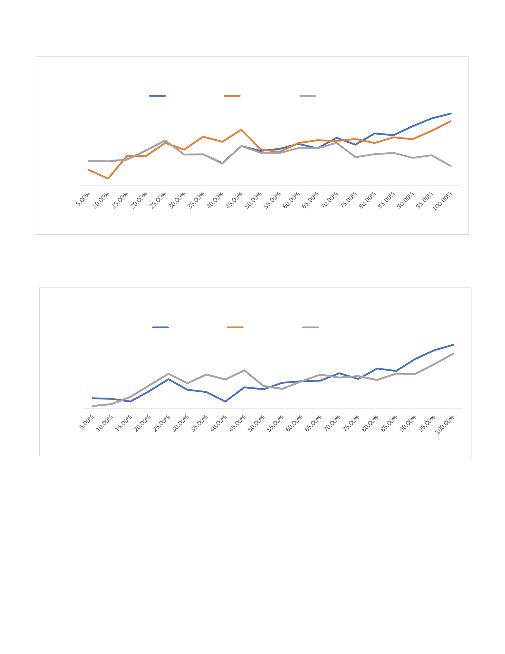
Figure 17 is visual representation for the commercial projects highlights the accuracy

comparison when the performance factor is set to SCI.

5.4 The Analysis of Educational Projects.

In the case of educational projects, the Earned Duration method achieves the highest

overall percentage. Additionally, when the performance factor is set to SPI and SCI, Earned

Duration maintains its supremacy. However, under the condition of a performance factor equal

to 1, Earned Schedule exhibits the highest accuracy. The upcoming visual representation will

provide a thorough overview of accuracy percentages across project duration percentages for

performance factors 1, SPI, SCI, and the average.

60%

65%

70%

75%

80%

85%

90%

95%

100%

Accuracy

Duration Percentage

EAR NED S C HE DULE VS EAR NED D UR ATION VS PLANNE D

DURATION AT PF =S C I (C OMM ETR IAL PROJ ECTS)

Earned Duration Earned Schedule Planned Value

55%

60%

65%

70%

75%

80%

85%

90%

95%

100%

Accuracy

Duration Percentage

EAR NED S CHEDULE VS EAR NED DUR ATIO N VS PLANNE D

DURATION AT PF =S P I (COMM ETRIAL PR OJ EC T S)

Earned Duration Earned Schedule Planned Value

Figure 16 Average Earned Schedule vs Earned duration vs Planned duration (Commercial Projects) at PF = SPI

Figure 17 Average Earned Schedule vs Earned duration vs Planned duration (Commercial Projects) AT PF = SCI

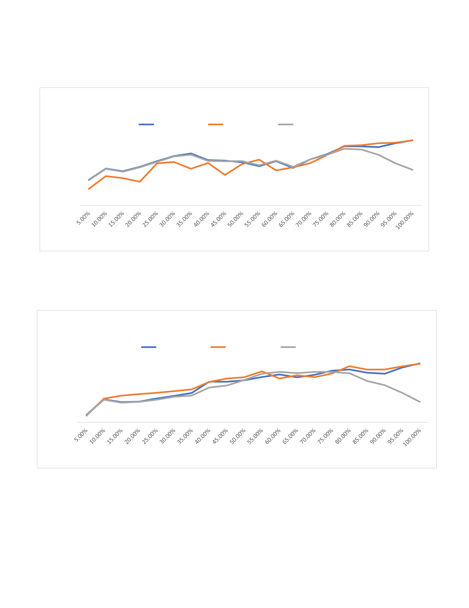
Figure 18 depiction showcases the comparison of accuracy among the three methods

on an average scale.

Figure 19 illustrates the accuracy comparison among the three methods under the

condition of a performance factor set to 1.

Figure 20 presents the accuracy comparison among the three methods when the

performance factor is set to SPI.

60%

65%

70%

75%

80%

85%

90%

95%

100%

Accuracy

Duration Percentage

AVER AGE E ARN ED S CHEDULE VS E ARNE D DUR ATION VS

PLANNE D DUR ATIO N (ED UCTIO NA L PRO J EC TS)

Earned Duration Earned Schedule Planned Value

70%

75%

80%

85%

90%

95%

100%

Accuracy

Duration Percentage

EARNED SC HE DULE VS EAR NED DUR ATION VS PLA NNED

DURATION AT PF =1 ( E DUC TIONAL PROJ EC TS )

Earned Duration Earned Schedule Planned Value

Figure 18 Average Earned Schedule vs Earned duration vs Planned duration (Educational projects)

Figure

Earned Schedule vs Earned duration vs Planned duration at

=1 (Educational projects)

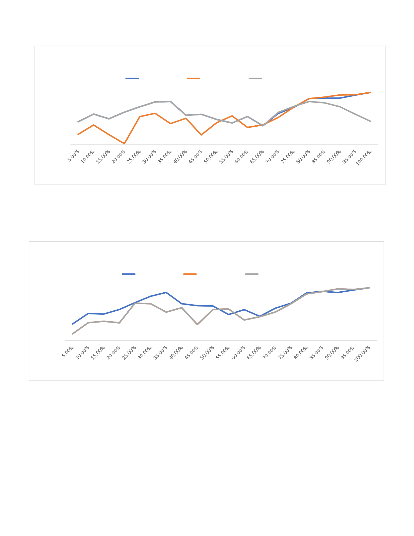
Figure 21 is the visual representation for the commercial projects underscores the

accuracy comparison when the performance factor is set to SCI.

5.5 The Analysis of Residential Projects.

For residential projects, in contrast to other projects, the Earned Schedule method secures the

highest overall percentage. Furthermore, under the conditions of a performance factor set to 1,

SPI, and SCI, the upcoming visual representation will deliver a comprehensive overview of

accuracy percentages across project duration percentages for performance factors 1, SPI, SCI,

and the average.

65%

70%

75%

80%

85%

90%

95%

100%

Accuracy

Duration Percentage

EARNED SC HE DULE VS EARNED DUR ATION VS PLA NNED

DURATION AT PF = SP I (EDU C TIONAL PROJ EC TS)

Earned Duration Earned Schedule Planned Value

60%

65%

70%

75%

80%

85%

90%

95%

100%

Accuracy

Duration Percentage

EAR NED S C HEDULE VS EARNED DUR ATIO N VS PLANNE D

DURATION AT P F = SCI (EDUCTIO NA L PROJ ECT S)

Earned Duration Earned Schedule Planned Value

Figure 20 Earned Schedule vs Earned duration vs Planned duration (Educational projects) at PF = SPI

Figure 21 Earned Schedule vs Earned duration vs Planned duration (Educational projects) AT PF = SCI

Figure 22 highlights the comparison of accuracy among the three methods on an

average scale.

Figure 23 illustrates the comparison of accuracy among the three methods when the

performance factor is set to 1.

Figure 24 showcases the accuracy comparison among the three methods when the performance

factor is configured to SPI.

60%

65%

70%

75%

80%

85%

90%

95%

100%

Accuracy

Duration Percentage

AVER AGE EARNE D S CHEDULE VS EA RNE D DUR ATION VS

PLANNE D DUR ATIO N (RES IDNETIAL PR OJ ECT S)

Earned Duration Earned Schedule Planned Value

65%

70%

75%

80%

85%

90%

95%

100%

Accuracy

Duration Percentage

EARNED SC HEDULE VS EARNED DUR ATIO N VS P LANNED

DURATION AT PF = 1(R ES ID NET IAL PROJ ECTS )

Earned Duration Earned Schedule Planned Value

Figure 22Average Earned Schedule vs Earned duration vs Planned duration (Residential projects)

Figure

Average Earned Schedule vs Earned duration vs Planned duration (Residential projects)

AT PF = 1

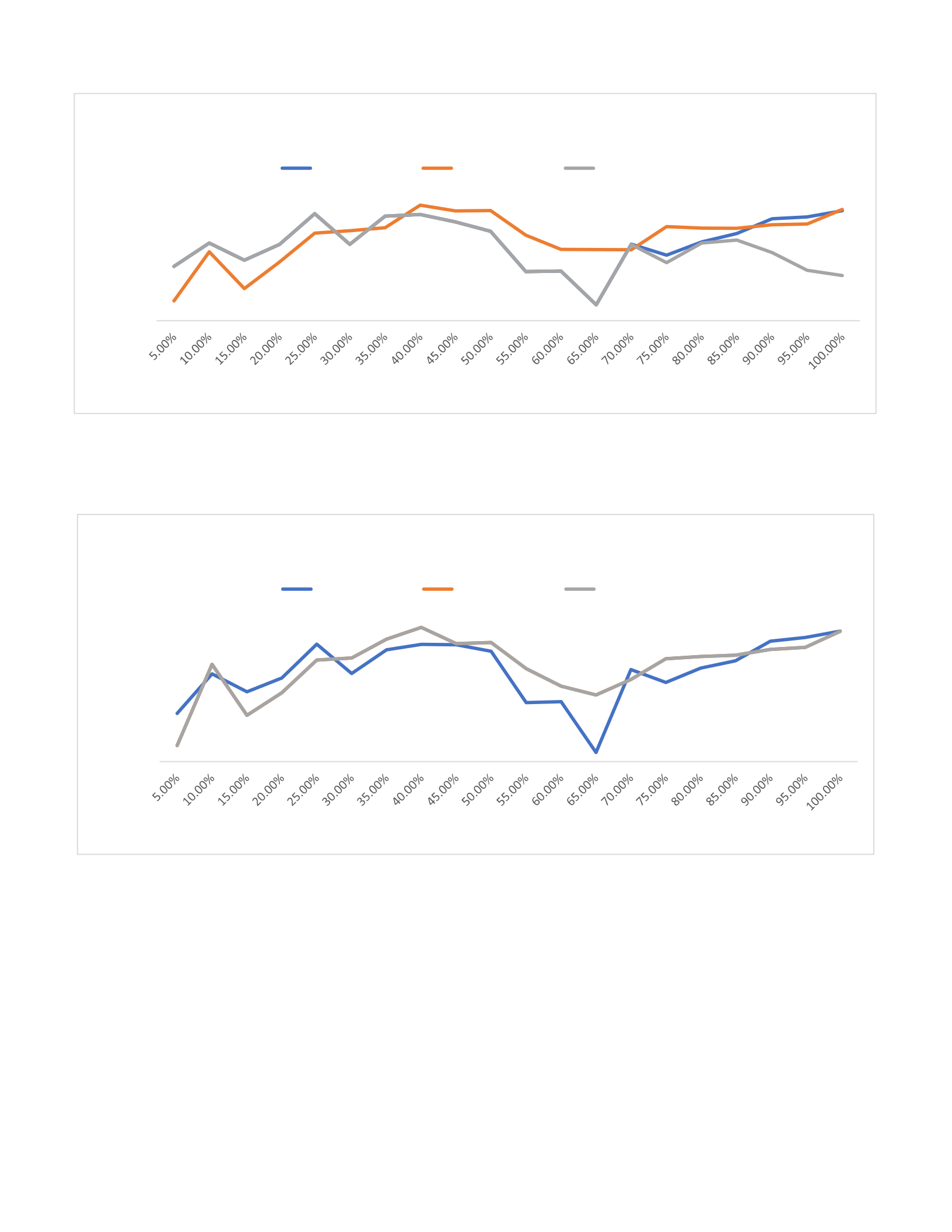
Figure 25 is the visual representation for commercial projects emphasizes the accuracy

comparison when the performance factor is set to SCI.

5.6 The Analysis of Renovation Projects.

In renovation endeavours, much like residential projects, the Earned Schedule method

consistently achieves the highest overall percentage. Additionally, when the performance

factor is set to 1, the earned duration takes precedence, while equality between the performance

factor, SPI, and SCI results in the earned duration coming out on top. A forthcoming visual

55%

60%

65%

70%

75%

80%

85%

90%

95%

100%

Accuracy

Duration Percentage

EAR NED S CHEDULE VS EAR NED DUR ATIO N VS PLANNE D

DURATION AT PF =S CI (RESID NETIAL P ROJ ECT S)

Earned Duration Earned Schedule Planned Value

Figure 25 Earned Schedule vs Earned duration vs Planned duration (Residential projects) AT PF = SCI

60%

65%

70%

75%

80%

85%

90%

95%

100%

Accuracy

Duration Percentage

EARNED SC HEDULE VS EARNED DUR ATIO N VS P LANNED

DURATION AT P F = SP I (RE SIDN ET IAL PR OJEC TS)

Earned Duration Earned Schedule Planned Value

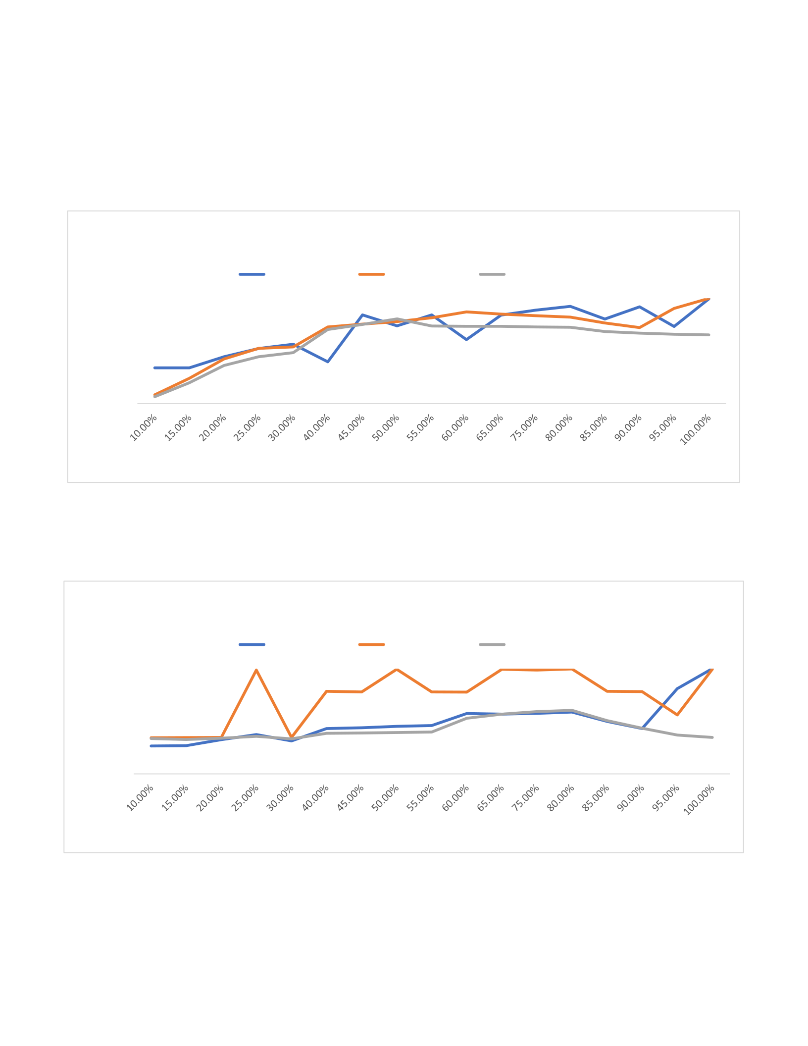
representation will provide a comprehensive overview of accuracy percentages across project

duration percentages for performance factors 1, SPI, SCI, and the average.

Figure 26 emphasizes the comparison of accuracy among the three methods on an average

scale.

Figure 27 depicts a comparison of accuracy among the three methods under the condition of a

performance factor set to 1.

Figure 28 displays a comparison of accuracy among the three methods under the configuration

of the performance factor to SPI.

80%

85%

90%

95%

100%

Accuracy

Duration Percentage

AVER AGE E ARN ED S CHEDULE VS E ARNE D DUR ATION VS

PLANNE D DUR ATION (R EN O VATIO N P ROJEC TS )

Earned Duration Earned Schedule Planned Value

90%

95%

100%

Accuracy

Duration Percentage

EAR NED S CHEDULE VS EAR NED DUR ATIO N VS PLANNE D

DURATION AT P F = 1(RE NO VATIO N PRO J ECT S)

Earned Duration Earned Schedule Planned Value

Figure 26 Average Earned Schedule vs Earned duration vs Planned duration (Renovation projects)

Figure 27 Earned Schedule vs Earned duration vs Planned duration (Renovation projects) AT PF =1

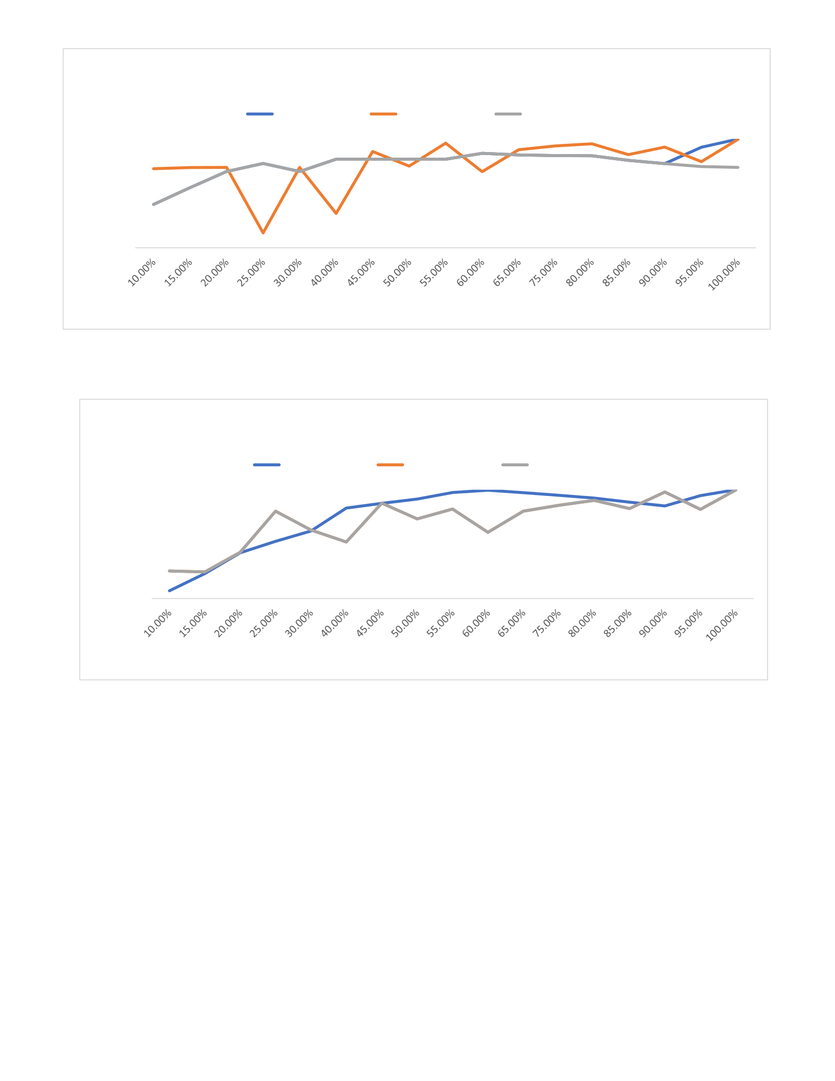
Figure 29 is the visual representation for commercial projects emphasizes the accuracy

comparison when the performance factor is set to SCI.

In summary, the analysis of various project types reveals distinct patterns in the

performance of Earned Duration and Earned Schedule methods under different performance

factors. In industrial projects, Earned Duration consistently secures the highest overall

percentage, except when the performance factor is set to SPI, where Earned Schedule excels in

accuracy. A similar trend is observed in commercial projects, with Earned Duration dominating

overall and Earned Schedule leading under the SPI performance factor. Educational projects

showcase a nuanced scenario, where Earned Duration performs best overall but Earned

Schedule surpasses under a performance factor set to 1. Notably, residential and renovation

projects deviate from the general pattern, with Earned Schedule emerging as the method with

the highest overall percentage. The detailed visual representations across project duration

75%

80%

85%

90%

95%

100%

Accuracy

Duration Percentage

EARNED SC HEDULE VS EARNED DUR ATIO N VS P LANNED

DURATION AT P F = SP I ( RE NOVATION PROJ ECTS)

Earned Duration Earned Schedule Planned Value

65%

70%

75%

80%

85%

90%

95%

100%

Accuracy

Duration Percentage

EARNED SC HE DULE VS EARNED DUR ATION VS PLA NNED

DURATION AT PF = SC I (RENOVATION P ROJ EC TS)

Earned Duration Earned Schedule Planned Value

Figure 28 Average Earned Schedule vs Earned duration vs Planned duration (Renovation projects) AT PF = SPI

Figure 29 Average Earned Schedule vs Earned duration vs Planned duration (Renovation projects) AT PF = SCI

percentages and performance factors 1, SPI, SCI, and the average offer a comprehensive

overview, aiding in understanding the nuanced dynamics of accuracy across diverse project

types and conditions.

5.7 International and domestic project managers

Another crucial criterion employed for the analysis involves assessing the accuracy by

comparing projects managed by international and domestic project managers. This aims to

underscore potential disparities between these two factors. Table 3 illustrates the variance in

accuracy between domestic and international project managers when using performance factor

equal to 1. As depicted in the table, projects led by international project managers consistently

exhibit higher accuracy levels compared to those overseen by domestic counterparts throughout

the project timeline.

Table 3 Comparison between international and domestic project managers when performance

factor equal to 1

Table 4 presents the discrepancy in accuracy between domestic and international

project managers when utilizing the performance factor equivalent to SPI. As indicated in the

table, projects supervised by international project managers consistently demonstrate higher

accuracy levels in comparison to those managed by domestic counterparts throughout the

project timeline.

Duration %

PM Accuracy At PF = 1 PM Accuracy At PF = 1

International

75.23% 74.37% 74.64% Domestic

64.58%

64.50% 64.40%

10%

International

74.63% 75.06% 73.15%

Domestic

69.82%

70.82% 69.48%

15%

International

79.06% 81.04% 76.92%

Domestic

68.53%

70.21% 68.47%

20%

International

75.05% 75.40% 72.52% Domestic

69.56%

71.84% 69.38%

25%

International

78.74% 78.90% 76.18% Domestic

75.17%

76.17% 74.04%

30%

International

77.86% 73.94% 74.78% Domestic

75.34%

74.69% 74.51%

35%

International

78.54% 77.11% 74.61% Domestic

77.18%

75.77% 76.85%

40%

International

82.40% 80.71% 78.59% Domestic

81.71%

80.75% 81.47%

45%

International

85.06% 84.10% 81.32% Domestic

81.62%

82.03% 81.49%

50%

International

84.98% 81.05% 82.80% Domestic

84.74%

85.16% 84.12%

55%

International

87.67% 81.11% 86.63% Domestic

85.91%

86.38% 85.46%

60%

International

88.11% 84.76% 85.47%

Domestic

86.10%

85.62% 84.48%

65%

International

89.99% 86.79% 85.75%

Domestic

88.38%

89.92% 86.14%

70%

International

89.01% 85.75% 83.15% Domestic

90.65%

89.32% 84.47%

75%

International

92.19% 89.32% 83.78% Domestic

91.18%

90.40% 82.77%

80%

International

93.22% 90.59% 84.12% Domestic

92.44%

92.55% 80.39%

85%

International

93.64% 94.11% 81.25% Domestic

93.27%

92.32% 78.77%

90%

International

95.80% 95.55% 77.61% Domestic

93.59%

94.28% 74.19%

95%

International

97.56% 96.91% 72.71% Domestic

96.42%

96.41% 73.68%

100%

International

99.18% 98.93% 70.56% Domestic

99.12%

98.79% 68.22%

Table 4 Comparison between international and domestic project managers when performance factor equal to 1

Table 5 displays the variation in accuracy between domestic and international project

managers, utilizing the performance factor equivalent to SCI. As outlined in the table, projects

overseen by international project managers consistently showcase higher accuracy levels

compared to those managed by their domestic counterparts across the project timeline.

Duration %

PM Accuracy At PF = SPI PM Accuracy At PF = SPI

International 72.43% 71.29% 72.43% Domestic

68.04%

64.21% 68.04%

10%

International 79.15% 64.98% 79.15% Domestic

73.79%

69.60% 73.79%

15%

International 80.29% 71.99% 80.29% Domestic

72.99%

74.13% 72.99%

20%

International

82.68% 86.37% 82.68%

Domestic

77.00%

71.44% 77.00%

25%

International

81.69% 86.27% 81.69%

Domestic

85.55%

79.28% 85.55%

30%

International

78.78% 76.75% 78.78%

Domestic

77.70%

85.81% 77.70%

35%

International

85.51% 86.51% 85.51% Domestic

76.15%

85.82% 76.15%

40%

International 83.67% 84.67% 83.67% Domestic

75.67%

84.62% 75.67%

45%

International 81.23% 83.28% 81.23% Domestic

81.33%

85.24% 81.30%

50%

International 79.48% 80.37% 79.48% Domestic

80.62%

79.38% 80.39%

55%

International 77.62% 85.78% 77.34% Domestic

79.49%

79.31% 79.36%

60%

International 75.36% 79.48% 73.85% Domestic

82.81%

81.99% 82.37%

65%

International 77.53% 81.77% 75.90% Domestic

81.23%

81.19% 80.18%

70%

International

86.18% 86.78% 79.97%

Domestic

84.85%

85.36% 81.42%

75%

International

87.12% 88.50% 78.65%

Domestic

82.85%

84.44% 75.89%

80%

International

91.28% 88.28% 82.89%

Domestic

88.36%

85.16% 78.26%

85%

International

92.69% 92.67% 81.53% Domestic

87.07%

87.46% 74.54%

90%

International 95.88% 93.67% 78.54% Domestic 92.23%

89.62% 74.18%

95%

International 97.80% 95.41% 72.92% Domestic 96.01%

93.61% 74.19%

100%

International 99.19% 98.63% 70.51% Domestic 99.11%

97.79% 68.22%

Duration %

PM Accuracy At PF = SCI PM Accuracy At PF = SCI

International

66.08% 66.47% 66.47% Domestic

63.58%

61.67% 61.67%

10%

International

73.66% 68.51% 68.51% Domestic

69.74%

69.10% 69.10%

15%

International

71.55% 65.62% 65.62% Domestic

68.41%

70.52% 70.52%

20%

International

76.57% 82.89% 82.89% Domestic

73.04%

72.14% 72.14%

25%

International

76.35% 81.58% 81.58%

Domestic

82.34%

82.69% 82.69%

30%

International

75.75% 73.82% 73.82%

Domestic

76.58%

86.36% 86.36%

35%

International

83.68% 81.07% 81.07% Domestic

75.00%

84.41% 84.41%

40%

International

80.78% 79.37% 79.37% Domestic

74.97%

83.53% 83.53%

45%

International

76.90% 76.94% 76.94% Domestic

79.48%

82.05% 82.05%

50%

International

76.99% 77.55% 77.55% Domestic

80.35%

78.46% 78.46%

55%

International

76.29% 80.57% 80.57% Domestic

78.15%

77.60% 77.60%

60%

International

72.44% 74.56% 74.56% Domestic

80.35%

79.20% 79.20%

65%

International

75.84% 77.77% 77.77% Domestic

80.85%

79.19% 79.19%

70%

International

85.03% 84.10% 84.10% Domestic

83.19%

83.95% 83.95%

In conclusion, the analysis of accuracy in project management, considering 1, SPI and SCI

performance factors, revealed consistent trends when comparing projects led by international

and domestic project managers. Tables 3, 4, and 5 consistently demonstrate that projects

supervised by international project managers consistently exhibit higher accuracy levels than

those managed by domestic counterparts throughout the entire project timeline. This

underscores a notable pattern suggesting that international project managers tend to achieve

higher accuracy in project execution, emphasizing the significance of managerial expertise in

achieving project objectives.

5.8 Guidelines Derived from the Above.

Following an in-depth analysis and meticulous calculations for project types, the subsequent

phase involves extending our scrutiny to encompass the collective results derived from thirty

distinct projects. This comprehensive examination aims to unveil overarching patterns and

insights, shedding light on the most effective method for projecting project completion dates.

Through a nuanced exploration of various facets and project durations, we endeavour to distil

valuable conclusions that will serve as practical guidance for optimizing the accuracy of project

forecasting methods.

 First and foremost, the Earned Duration method emerged as the most accurate among the

three techniques across various metrics, including average accuracy, performance factor set

to 1, and performance factor set to SPI Earned Schedule were the highest. However, under

the performance factor set to SCI, both Planned Duration and Earned Schedule surpassed

Earned Duration, achieving an accuracy of 81.52%%. This underscores the Earned

Duration method's exceptional efficacy in predicting project completion dates across a

diverse spectrum of project types and durations.

75%

International

85.51% 84.60% 84.60%

Domestic

81.28%

81.84% 81.84%

80%

International

88.98% 85.44% 85.44%

Domestic

87.37%

83.48% 83.48%

85%

International

90.01% 91.64% 91.64% Domestic

85.73%

85.53% 85.53%

90%

International 94.42% 92.60% 92.60% Domestic 91.91%

88.72% 88.72%

95%

International 97.24% 95.04% 95.04% Domestic 95.87%

93.11% 93.11%

100%

International 99.13% 98.57% 98.57% Domestic 99.12%

97.70% 97.70%

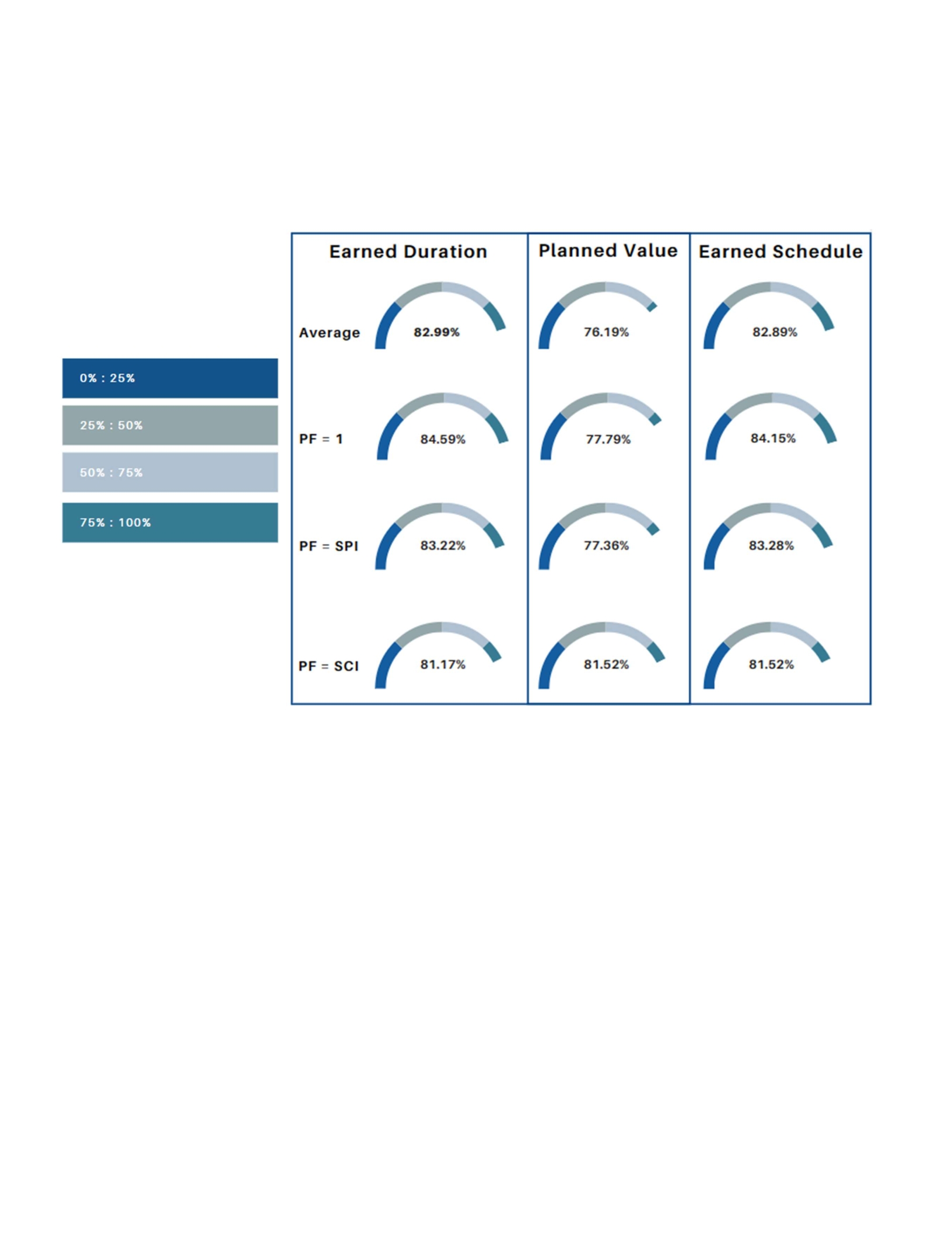
In Figure 30, the variation in average accuracy achieved by each method is illustrated. The

gauge chart displays four categories, ranging from 0 to 25%, 25% to 50%, 50% to 75%, and

finally, 75% to 100%, with each category represented by a distinct color as shown below.

 Furthermore, the thesis unveiled a useful guideline for selecting the most efficient

technique based on project duration percentages. These guidelines will assist project

managers and practitioners in making informed decisions about which technique to employ

for the most accurate project forecasting in general:

1- For projects with a duration ranging from 0% to 20% of the total project timeline,

the Earned Duration method is recommended.

2- In the case of projects spanning from 20% to 50% of the project duration, the Earned

Schedule method is the optimal choice.

3- Projects in the 55% to 65% duration range are best suited for the Earned Duration

method.

Figure 30 Overall accuracy achieved per method.

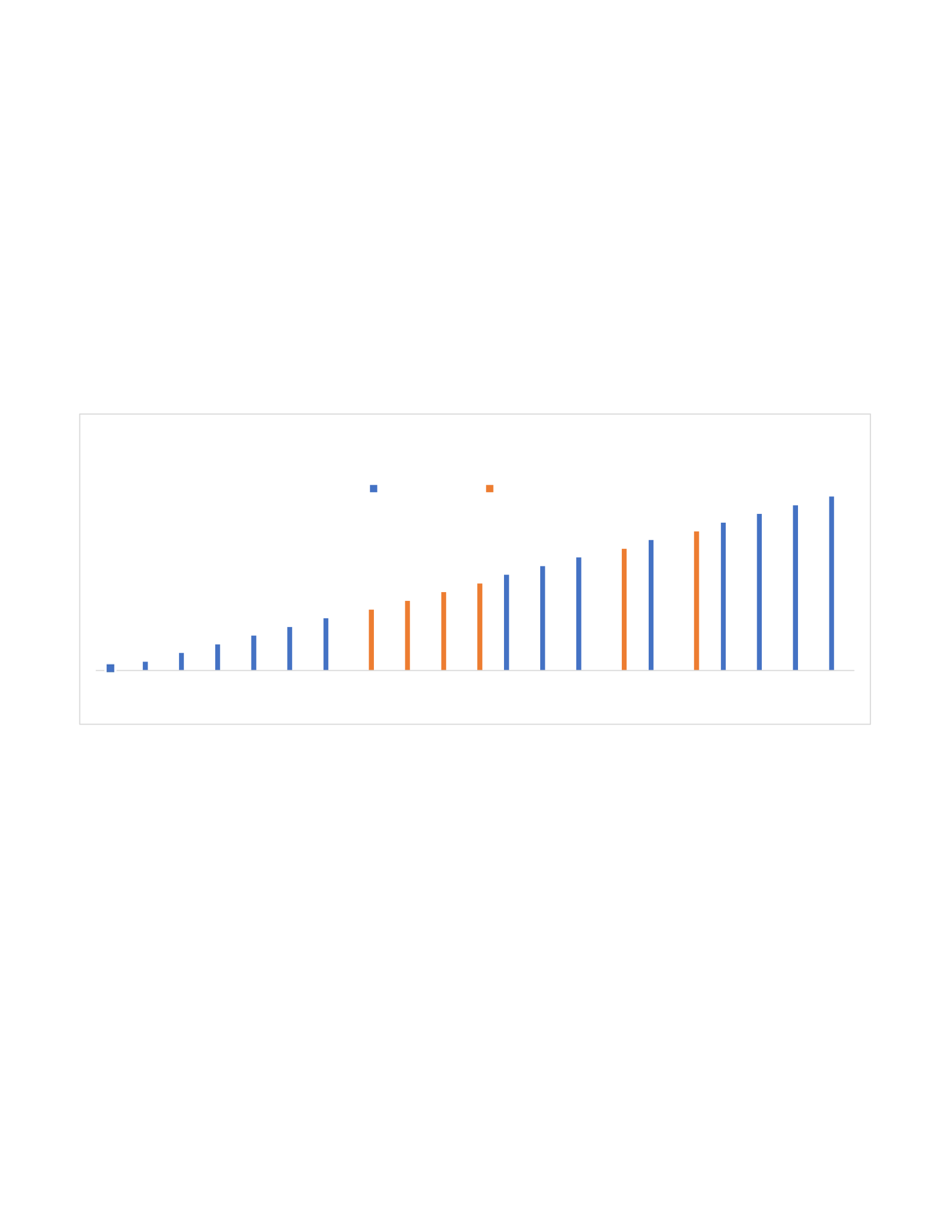
4- Between 65% and 70% of the project timeline, the Earned Schedule method proves

to be the most efficient.

5- For projects from 70% to 75% of their duration, the Earned Duration method is once

again the recommended technique.

6- In the 75% to 80% project duration range, the Earned Schedule method is the most

effective.

7- Finally, for projects nearing completion, from 80% to 100% of the project duration,

the Earned Duration method is the superior choice.

Figure 31 illustrates the best method to use over the project duration percentage as mentioned

above.

Additionally, the thesis introduced a practical guideline for selecting the most effective

technique based on project duration percentages. These recommendations are designed to aid

project managers and practitioners in making well-informed decisions regarding the choice of

techniques for precise project forecasting when using a performance factor equal to 1:

1- For projects constituting 0% to 5% of the total project timeline, it is advisable to use

the Earned Duration method.

2- Projects with a duration falling within the 5% to 30% range of the total project timeline

are best suited for the Earned Schedule method.

3- Optimal results are achieved with the Earned Duration method for projects spanning

from 30% to 60% of the project duration.

Figure 31 Comparison Between Earned Duration vs Earned Schedule over the project duration Percentage.

0 % 5 % 1 0 % 1 5 % 2 0% 2 5 % 3 0 % 3 5 % 4 0 % 4 5 % 5 0 % 5 5 % 6 0% 6 5 % 7 0 % 7 5 % 8 0% 8 5 % 9 0 % 9 5 % 1 0 0 %

DURATION PERCENTAGE

COM PARISON BE TWEE N E AR NED DURATIO N VS EAR NED

SCHED U LE OVER THE P ROJ EC T DU RAT ION P ERC ENTAGE

Earned Duration Earned Schedule

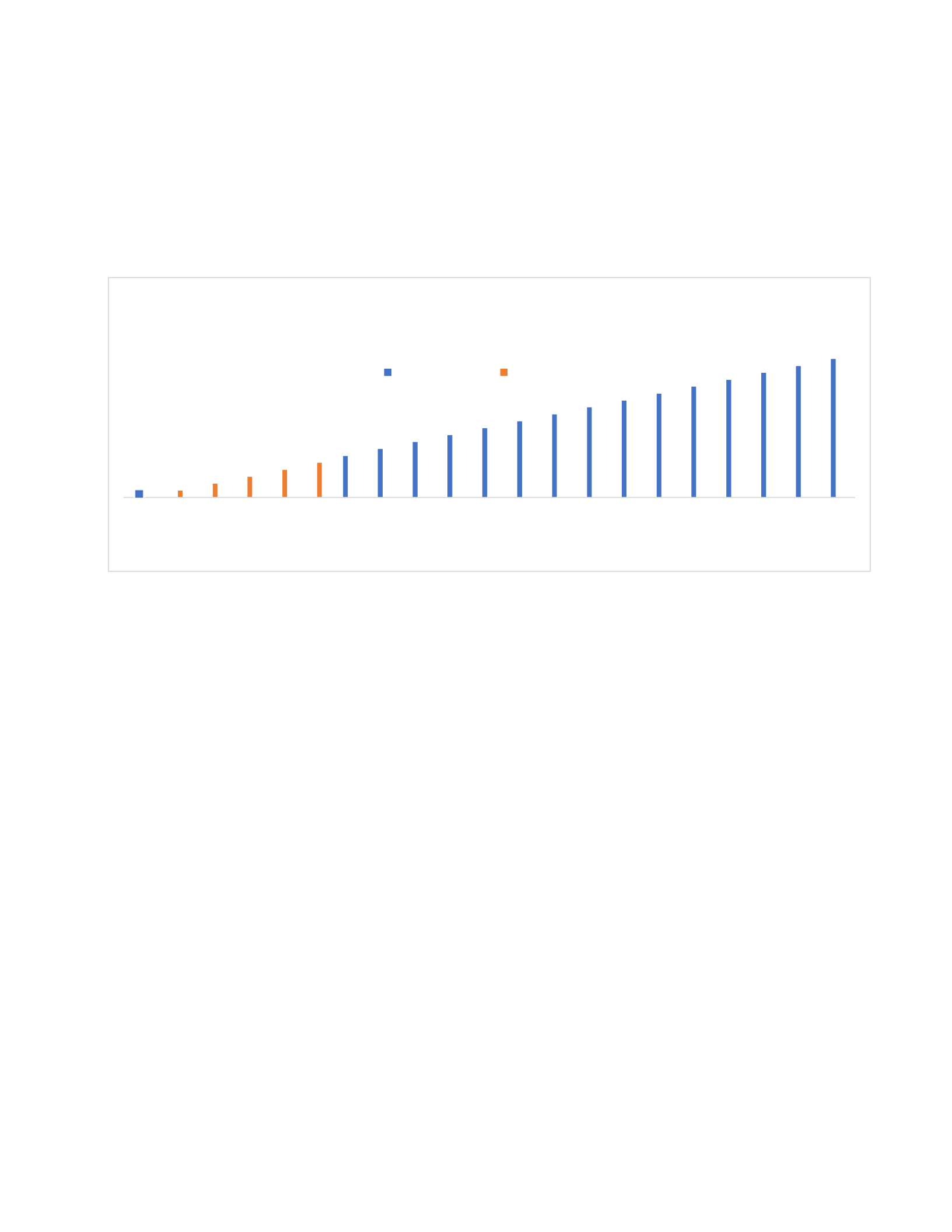
4- Projects with a duration ranging from 65% to 70% are most appropriately managed

using the Earned Schedule method.

5- Between 70% and 100% of the project timeline, the Earned Duration method

demonstrates the highest efficiency.

Figure 32 depicts the overall outcome when the performance factor is set to 1.

Moreover, the thesis introduced a valuable guideline for selecting the most effective

technique based on project duration percentages. These recommendations aim to assist project

managers and practitioners in making well-informed decisions regarding the choice of

techniques for accurate project forecasting, particularly when employing the performance

factor SPI:

1. It is advisable to use the Earned Duration method for projects constituting 0% to 30%

of the total project timeline.

2. Projects with a duration falling within the 30% to 65% range of the total project timeline

are most suitable for the Earned Schedule method.

3. Optimal results are attained with the Earned Duration method for projects spanning

from 65% to 70% of the project duration.

4. Projects with a duration ranging from 70% to 75% are best managed using the Earned

Schedule method.

5. Between 75% and 100% of the project timeline, the Earned Duration method

demonstrates the highest efficiency.

Figure 32 Comparison Between Earned Duration vs Earned Schedule over the project duration Percentage.

0% 5% 1 0% 1 5% 2 0 % 2 5 % 3 0 % 3 5 % 40 % 4 5% 50 % 5 5 % 60 % 6 5% 70 % 7 5 % 8 0% 8 5 % 90% 9 5 % 1 0 0 %

DURATION PERCENTAGE

COM PARISON BE TWEE N E AR NED DURATIO N VS EAR NED

SCHED U LE OVER THE P ROJ EC T DU RAT ION PE RC ENTAGE AT

PF = 1

Earned Duration Earned Schedule

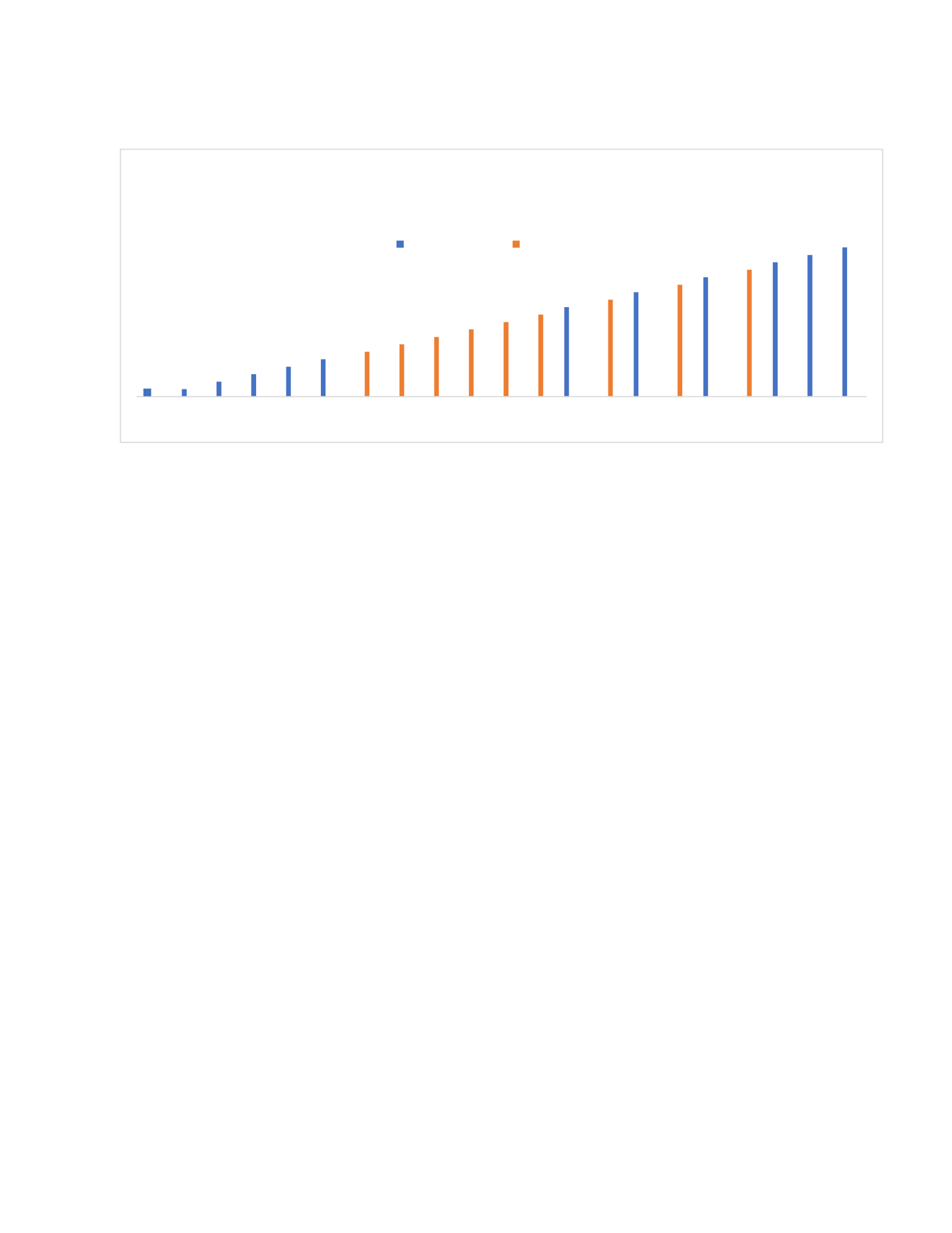
Figure 33 illustrates the overall outcome when the performance factor is configured to SPI.

The selection of techniques for precise project forecasting when utilizing the performance

factor SPI multiplied by CPI:

1. It is recommended to employ the Earned Duration method for projects encompassing

0% to 15% of the total project timeline.

2. Projects with a duration ranging from 15% to 55% of the total project timeline are most

appropriately managed using the Earned Schedule method.

3. Optimal outcomes are achieved with the Earned Duration method for projects spanning

from 55% to 60% of the project duration.

4. Projects with a duration falling within the 60% to 65% range are most effectively

handled through the Earned Schedule method.

5. Between 65% and 70% of the project timeline, the Earned Duration method

demonstrates the highest efficiency.

6. Within the 70% to 75% duration range, the Earned Schedule method exhibits the

highest efficiency.

7. For projects constituting 75% to 100% of the project timeline, the Earned Duration

method demonstrates the highest efficiency.

Figure

Comparison Between Earned Duration vs Earned Schedule over the project duration Percentage AT PF = SPI

0 % 5 % 1 0 % 1 5 % 2 0% 2 5 % 3 0 % 3 5 % 4 0 % 4 5 % 5 0% 5 5 % 60 % 6 5 % 7 0 % 7 5 % 8 0% 8 5 % 9 0 % 9 5 % 1 0 0%

DURATION PERCENTAGE

COMPARIS ON BE TW E EN EAR NED DURATION VS E AR NED

SC HE D ULE OVER THE P ROJEC T DU RATION PE RC EN TA GE AT

PF = S PI

Earned Duration Earned Schedule

Figure 34 depicts the overall outcome when the performance factor is set to SCI.

 The analysis considered each technique based on three essential performance factors:

Performance Factor (PF) equal to 1, PF equal to Schedule Performance Index (SPI), and

PF equal to SPI multiplied by Cost Performance Index (CPI). The Average comparison

between the three methods is shown in figure 35.

Figure 35 Average comparison between Earned Schedule Vs Earned Duration Vs Planned Value

The findings from the projects indicate the following:

0 % 5 % 1 0 % 1 5 % 2 0% 2 5 % 3 0% 3 5 % 4 0 % 4 5 % 5 0 % 5 5 % 6 0 % 6 5 % 7 0 % 7 5% 8 0 % 8 5 % 9 0 % 9 5 % 1 0 0 %

DURATION PERCENTAGE

COM PARISON BE TWEE N E AR NED DURATIO N VS EAR NED

SCHED U LE OVER THE P ROJ EC T DU RAT ION PE RC ENTAGE AT

PF = SC I

Earned Duration Earned Schedule

Figure 34 Comparison Between Earned Duration vs Earned Schedule over the project duration Percentage AT PF = SCI.

60.00%

70.00%

80.00%

90.00%

100.00%

Accuracy

Duration Percentage

Average comparison between Earned Schedule Vs Earned

Duration Vs Planned Value

Earned Duration Earned Schedule Planned Value

1- When evaluating the performance factor (PF) as 1, or simply assessing whether projects

were completed on schedule without considering cost and schedule performance, the

Earned Duration method consistently emerged as the superior technique with 98.88%

very close to earned schedule percentage which is 98.71% as shown in figure 36.

2- Similarly, when focusing solely on the Schedule Performance Index (SPI), which

measures schedule adherence regardless of cost performance, the Earned Duration

method consistently displayed the highest accuracy as shown in figure 37.

60.00%

65.00%

70.00%

75.00%

80.00%

85.00%

90.00%

95.00%

100.00%

Axis Title

Earned Schedule Vs Earned Duration Vs Planned Value at PF = 1

Earned Duration Earned Schedule Planned Value

Figure 36 Earned Schedule Vs Earned Duration Vs Planned Value at PF = 1

Figure 37 Earned Schedule Vs Earned Duration Vs Planned Value at PF = SPI

60.00%

65.00%

70.00%

75.00%

80.00%

85.00%

90.00%

95.00%

100.00%

Axis Title

Earned Schedule Vs Earned Duration Vs Planned Value at PF = SPI

Earned Duration Earned Schedule Planned Value

3- Notably, when considering both schedule and cost performance together, represented

as PF = SPI x CPI, both the Earned Duration and Earned Schedule methods achieved

the same level of accuracy. This indicates that in scenarios where both schedule and

cost performance are vital considerations, these two methods provide equally reliable

results as shown in figure 38.

In a similar fashion, encompassing the project types, the subsequent outcomes were derived

from the examination of both industrial and commercial projects in table 4.

In industrial projects, the highest accuracy throughout the project duration is consistently

attained with the earned duration method, particularly when employing the performance factors

equal to SPI and one. In some instances, the earned schedule also emerges as a leading method.

Similarly, for commercial projects, the pattern is largely analogous to industrial projects, with

earned duration predominating in most phases of the project timeline. In the context of

educational projects, earned duration consistently secures the highest accuracy across a

significant portion of the project duration percentages, while earned schedule and planned

value take precedence in certain duration percentages. The overall outcomes are shown in table

4 which illustrates the methods and performance factors with highest accuracy according to

duration % and project industrial, commercial, and educational.

60.00%

65.00%

70.00%

75.00%

80.00%

85.00%

90.00%

95.00%

100.00%

Axis Title

Earned Schedule Vs Earned Duration Vs Planned Value at PF =

SCI

Earned Duration Earned Schedule Planned Value

Figure 38 Earned Schedule Vs Earned Duration Vs Planned Value at PF = SCI

Table 5 Industrial, commercial, and educational projects comparison based on duration percentage.

Similarly, considering the various project types, the subsequent results were obtained through

an analysis of both educational and renovation projects in table above. Finally, incorporating

the project types, the following results were obtained through the examination of renovation

projects. However, it should be noted that this may not be a robust measure, as only one project

was utilized in this analysis in table 6.

Table 6 method and performance factors with highest accuracy according to duration

% and project type (Educational and Residential)

Duration %

Type PF

Method

Accuracy

Type PF Method

Accuracy

Type PF

Method

Accuracy

5% Industrial

1 ED 61.91% Commercial

SPI

69.76%

Educational

SPI

79.76%

10% Industrial

SPI

ES 72.08% Commercial

SPI

ED 69.47% Educational

SPI

ED 84.76%

15% Industrial

SPI

ED 72.61% Commercial

SPI

ES 72.77% Educational

1 ES 83.11%

20% Industrial

SPI

ES 80.72% Commercial

SPI

ED 76.12% Educational

SPI

ED 86.00%

25% Industrial

SPI

ES 78.88% Commercial

SPI

82.09%

Educational

SPI

89.50%

30% Industrial

1 ES 73.94% Commercial

SPI

ES 76.57% Educational

SPI

ED 92.70%

35% Industrial

SCI

ED 83.90% Commercial

SPI

ES 84.46% Educational

SCI

ED 95.53%

40% Industrial

1 ED 77.18% Commercial

SPI

ES 81.29% Educational

1 ED 89.95%

45% Industrial

1 ED 79.57% Commercial

SPI

88.65%

Educational

91.52%

50% Industrial

1 ED 79.23% Commercial

1 ED 82.67% Educational

1 ES 92.10%

55% Industrial

SPI

ES 82.36% Commercial

1 ED 85.18% Educational

1 ES 95.02%

60% Industrial

1 ED 80.55% Commercial

1 ED 86.10% Educational

1 PV 94.74%

65% Industrial

SPI

ED 86.97% Commercial

1 ED 88.94% Educational

1 PV 94.10%

70% Industrial

SPI

ED 88.86% Commercial

1 ED 90.93% Educational

1 PV 94.75%

75% Industrial

SPI

ED 89.96% Commercial

91.56%

Educational

95.32%

80% Industrial

SPI

ED 90.66% Commercial

1 ED 92.76% Educational

1 ES 97.54%

85% Industrial

SCI

ES 93.80% Commercial

1 ED 93.50% Educational

SCI

ED 96.34%

90% Industrial

SPI

ED 93.98% Commercial

1 ED 93.10% Educational

SCI

ES 98.20%

95% Industrial

SPI

ED 96.61% Commercial

96.05%

Educational

97.67%

100% Industrial

SCI

ES 99.18% Commercial

SCI

ED 98.58% Educational

SCI

ED 98.98%

Duration

% Type PF Method

Accuracy

Type PF Method

Accuracy

Residential

SPI

77.52%

10%

Renovation

93.43%

10%

Residential

SCI

85.39%

15%

Renovation

93.45%

15%

Residential

SPI

79.52%

20%

Renovation

93.46%

20%

Residential

SPI

84.59%

25%

Renovation

99.86%

25%

Residential

SPI

94.52%

30%

Renovation

93.46%

30%

Residential

SPI

89.02%

40%

Renovation

97.84%

35%

Residential

SPI

93.73%

45%

Renovation

97.79%

40%

Residential

SPI

97.27%

50%

Renovation

99.94%

45%

Residential

SPI

95.36%

55%

Renovation

SCI

99.10%

50%

Residential

SPI

95.55%

60%

Renovation

SCI

99.85%

55%

Residential

92.48%

65%

Renovation

99.94%

60%

Residential

91.68%

75%

Renovation

99.87%

65%

Residential

92.76%

80%

Renovation

99.97%

70%

Residential

93.53%

85%

Renovation

97.84%

Table 6 Residential and renovation comparison based on duration percentage.

Ultimately, by integrating the various project types, the subsequent results were derived

through the comprehensive analysis of all projects, excluding consideration of specific project

types. In general, the earned duration method proves to be the most effective throughout nearly

the entire project duration. Concerning performance factors, it is generally advisable to utilize

the schedule performance index (SPI) for up to approximately 50% of the project duration.

Subsequently, employing the performance factor equal to 1 emerges as the preferred approach

to attain optimal results.

In conclusion to the discussion chapter, future research directions could involve

implementing the identified findings and assessing their accuracy. A valuable avenue for

exploration would be to compare the outcomes of this study with subsequent measurements,

75%

Residential

94.49%

90%

Renovation

SCI

99.26%

80%

Residential

95.45%

95%

Renovation

SCI

98.13%

85%

Residential

91.32%

100%

Renovation

100.00%

90%

Residential 1 ED 94.95%

95%

Residential 1 ED 95.05%

100%

Residential 1 ED 96.68%

Duration

% PF Method

Accuracy

SPI

68.36%

10%

SPI

74.25%

15%

SPI

73.59%

20%

SPI

77.84%

25%

SPI

83.64%

30%

SPI

79.74%

35%

SPI

84.19%

40%

SPI PV 83.66%

45%

SPI PV 85.48%

50%

1 ED 84.08%

55%

86.16%

60%

86.35%

65%

88.42%

70%

1 ED 90.05%

75%

1 ED 91.47%

80%

1 ED 92.60%

85%

1 ED 92.96%

90%

1 ED 93.79%

95%

1 ED 96.22%

100%

1 ED 98.42%

Table 7 Overall Projects highest accuracy achieved based on duration percentage.

analyzing any differences in accuracy between the initial and subsequent results. Additionally,

while the study delved into various EVM techniques and highlighted their limitations, future

research might explore alternative approaches for comparison.

Moreover, the study raises questions about the continued reliance on EVM,

emphasizing the need for proper improvements to potentially enhance the application of these

techniques in upcoming construction projects. It is worth noting that the research did not

address the construction of a model for future estimations, leaving room for further

investigation in this area.

The next chapter, Conclusion, will serve as the culmination of this research journey,

summarizing the essential discoveries, outlining practical implications, and suggesting avenues

for further exploration. Our exploration of EVM within the construction landscape will come

full circle, providing a comprehensive understanding that bridges theory and practice.

Chapter 6: Conclusion

the implementation of EVM within the Egyptian construction industry presents notable

challenges pertaining to application, accuracy, and result interpretability. Despite these

challenges, there exists a significant opportunity to leverage technological advancements and

develop a refined, controlled EVM approach that can markedly enhance project management

practices.

This research aims to contribute to this enhancement by conducting a thorough

evaluation of Earned Duration, Earned Schedule, and Planned Value methods in the context of

a diverse array of 30 construction projects across various sectors in Egypt. Spanning

commercial, educational, industrial, renovation, and residential domains, these projects were

analyzed for their accuracy in forecasting completion dates, with a focus on identifying the

most efficient method based on project duration percentages.

The comprehensive study covered a significant timeframe, from January 15, 2015, to

December 30, 2023, providing a robust foundation for the findings. Notably, the Earned

Duration method emerged as the most accurate technique across multiple metrics, including

average accuracy, performance factors set to 1 and SPI. However, under the performance factor

set to SCI, both Planned Duration and Earned Schedule surpassed Earned Duration,

emphasizing the need for nuanced considerations in method selection.

While Earned Duration consistently proved effective for industrial, commercial, and

educational projects, the Earned Schedule method outperformed in renovation and residential

contexts. The thesis not only shed light on the most accurate methods but also provided

practical guidelines for selecting techniques based on project duration percentages, offering

valuable insights for project managers in the Egyptian construction sector. The introduced

guidelines, tailored to different performance factors, serve as a roadmap for informed decision-

making, contributing to improved project forecasting accuracy and overall project management

practices. The applicability of these recommendations underscores the importance of aligning

the choice of technique with the unique characteristics of each construction project, thus

enhancing the reliability and efficiency of the forecasting process.

Furthermore, the investigation prompts inquiries regarding the ongoing dependence on

EVM, underscoring the necessity for substantial enhancements to potentially elevate the

efficacy of these techniques in forthcoming construction projects. Importantly, it is essential to

highlight that the study did not encompass projects beyond the geographical scope of Egypt.

Unlocking the potential of Earned Value management in construction: A Comparative Study

Students also viewed