


Chapter 1 Course Overview
Chapter 1
Course Overview
1.1 Goals for 6.01
We have many goals for this course. Our primary goal is for you to learn to appreciate and use the
fundamental design principles of modularity and abstraction in a variety of contexts from electrical
engineering and computer science. To achieve this goal, we will study electrical engineering (EE) and
computer science (CS) largely from the perspective of how to build systems that interact with, and attempt
to control, an external environment. Such systems include everything from low-level controllers like heat
regulators or cardiac pacemakers, to medium-level systems like automated navigation or virtual surgery,
to high-level systems that provide more natural human-computer interfaces.
Our second goal is to show you that making mathematical models of real systems can help in the design
and analysis of those systems; and to give you practice with the difficult step of deciding which aspects of
the real world are important to the problem being solved and how to model them in ways that give insight
into the problem.
We also hope to engage you more actively in the educational process. Most of the work of this course will
not be like typical problems from the end of a chapter. You will work individually and in pairs to solve
problems that are deeper and more open-ended. There will not be a unique right answer. Argument,
explanation, and justification of approach will be more important than the answer. We hope to expose
you to the ubiquity of trade-offs in engineering design: it is rare that an approach will be best in every
dimension; some will excel in one way, others in a different way. Deciding how to make such trade-offs is
a crucial part of engineering.
Another way in which we hope to engage you in the material is by having many of you return to the course
as lab assistants in future semesters. Having a large number of lab assistants in the class means that
students can be given more open-ended problems, and have people around to help them when they are
stuck. Even more importantly, the lab assistants are meant to question the students as they go; to
challenge their understanding and help them see and evaluate a variety of approaches. This process is of
great intellectual value to student and lab assistant alike.
Finally, of course, we have the more typical goals of teaching exciting and important basic material from
electrical engineering and computer science, including modern software engineering, linear systems

analysis, electronic circuits, and decision-making. This material all has an internal elegance and beauty, as
well as crucial role in building modern EE and CS systems.
1.2 Modularity, abstraction, and modeling
Whether proving a theorem by building up from lemmas to basic theorems to more specialized results, or
designing a circuit by building up from components to modules to complex processors, or designing a
software system by building up from generic procedures to classes to class libraries, humans deal with
complexity by exploiting the power of abstraction and modularity. Without such tools, a single person
would be overwhelmed by the complexity of a system, as there is only so much detail that a single person
can consciously manage at a time.
Modularity is the idea of building components that can be re-used; and abstraction is the idea that after
constructing a module (be it software or circuits or gears), most of the details of the module construction
can be ignored and a simpler description used for module interaction (the module computes the square
root, or doubles the voltage, or changes the direction of motion).
Given basic modules, one can move up a level of abstraction and construct a new module by putting
together several previously-built modules, thinking only of their abstract descriptions, and not their
implementations. And, of course, this process can be repeated over many stages. This process gives one
the ability to construct systems with complexity far beyond what would be possible if it were necessary to
understand each component in detail.
Any module can be described in a large number of ways. We might describe the circuitry in a digital watch
in terms of how it behaves as a clock and a stopwatch, or in terms of voltages and currents within the
circuit, or in terms of the heat produced at different parts of the circuitry. Each of these is a different model
of the watch. Different models will be appropriate for different tasks: there is no single correct model.
Rather, each model exposes different dimensions of the system, allowing us to explore many aspects of
the design space of a system, and to trade off different factors in the performance of a system.
The primary theme of this course will be to learn about different methods for building modules out of
primitives, and of building different abstract models of them, so that we can analyze or predict their
behavior, and so we can recombine them into even more complex systems. The same fundamental
principles will apply to software, to control systems, and to circuits.
1.2.1 Example problem
Imagine that you need to make a robot that will roll up close to a light bulb and stop a fixed distance from
it. The first question is, how can we get electrical signals to relate to the physical phenomena of light
readings and robot wheel rotations? There is a large part of electrical engineering related to the design of
physical devices that connect to the physical world in such a way that some electrical property of the
device relates to a physical process in the world. For example, a light-sensitive resistor (photo-resistor) is
a sensor whose resistance changes depending on light intensity impinging on it; a motor is an effector
whose rotor speed is related to the voltage across its two terminals. In this course, we will not examine
the detailed physics of sensors and effectors, but will concentrate on ways of designing systems that use
sensors and effectors to perform both simple and more complicated tasks. To get a robot to stop in front
of a light bulb, the problem will be to find a way to connect the photo-resistor to the motor, so that the

robot will stop at an appropriate distance from the bulb. Thus, we will already use the idea of abstraction
to treat sensors Chapter 1 Course Overview
and effectors as primitive modules whose internal details we can ignore, and whose performance
characteristics we can use as we design systems built on these elements.
1.2.2 An abstraction hierarchy of mechanisms
Given the light-sensitive resistor and the motor, we could find many ways of connecting them, using bits
of metal and ceramic of different kinds, or making some kind of magnetic or mechanical linkages. The
space of possible designs of machines is enormous.
One of the most important things that engineers do, when faced with a set of design problems, is to
standardize on a basis set of components to use to build their systems. There are many reasons for
standardizing on a basis set of components, mostly having to do with efficiency of understanding and of
manufacturing. It is important, as a designer, to develop a repertoire of standard bits and pieces of designs
that you understand well and can put together in various ways to make more complex systems. If you use
the same basis set of components as other designers, you can learn valuable techniques from them, rather
than having to re-invent the techniques yourself. And other people will be able to readily understand and
modify your designs.
We can often make a design job easier by limiting the space of possible designs, and by standardizing on:
• a basis set of primitive components;
• ways of combining the primitive components to make more complex systems;
• ways of “packaging” or abstracting pieces of a design so they can be reused (in essence creating
new “primitives”); and
• ways of capturing common patterns of abstraction (essentially, abstracting our abstractions).
Very complicated design problems can become tractable using such a primitive-combinationabstraction-
pattern (PCAP) approach. In this class, we will examine and learn to use a variety of PCAP strategies
common in EE and CS, and will even design some of our own, for special purposes. In the rest of this
section, we will hint at some of the PCAP systems we will be developing in much greater depth throughout
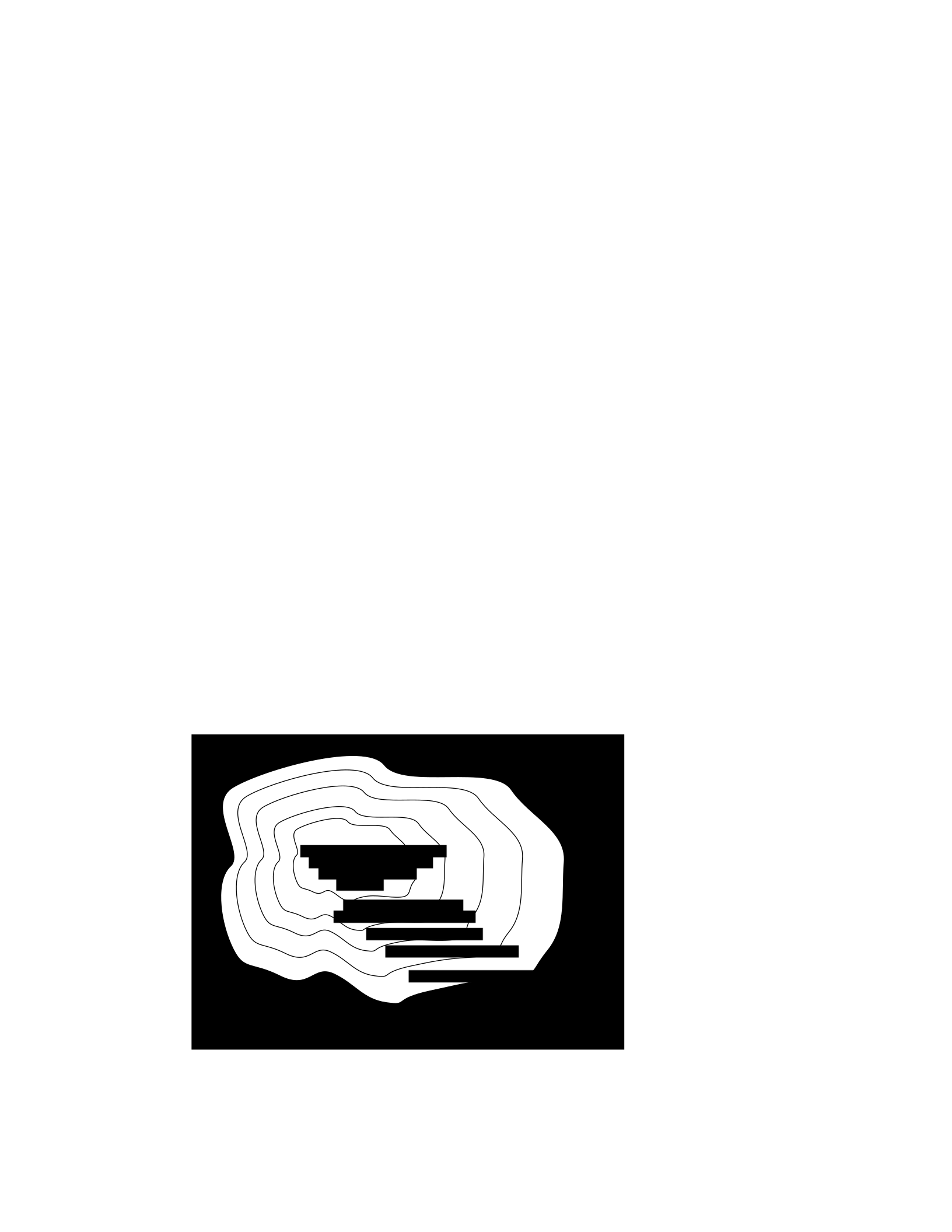
the class. Figure 1.1 shows one view of this development, as a successive set of restrictions of the design
space of mechanisms.
One very important thing about abstract models is that once we have fixed the abstraction, it will usually
be possible to implement it using a variety of different underlying substrates. So, as shown in figure 1.2,
we can construct general-purpose computers out of a variety of different kinds of systems, including digital
circuits and general-purpose computers. And systems satisfying the digital circuit abstraction can be
constructed from analog circuits, but also from gears or water or light.
Another demonstration of the value of abstracted models is that we can use them, by analogy, to describe
quite different systems. So, for example, the constraint models of circuits that we will study can be applied
to describing transmission of neural signals down the spinal cord, or of heat through a network of
connected bodies.
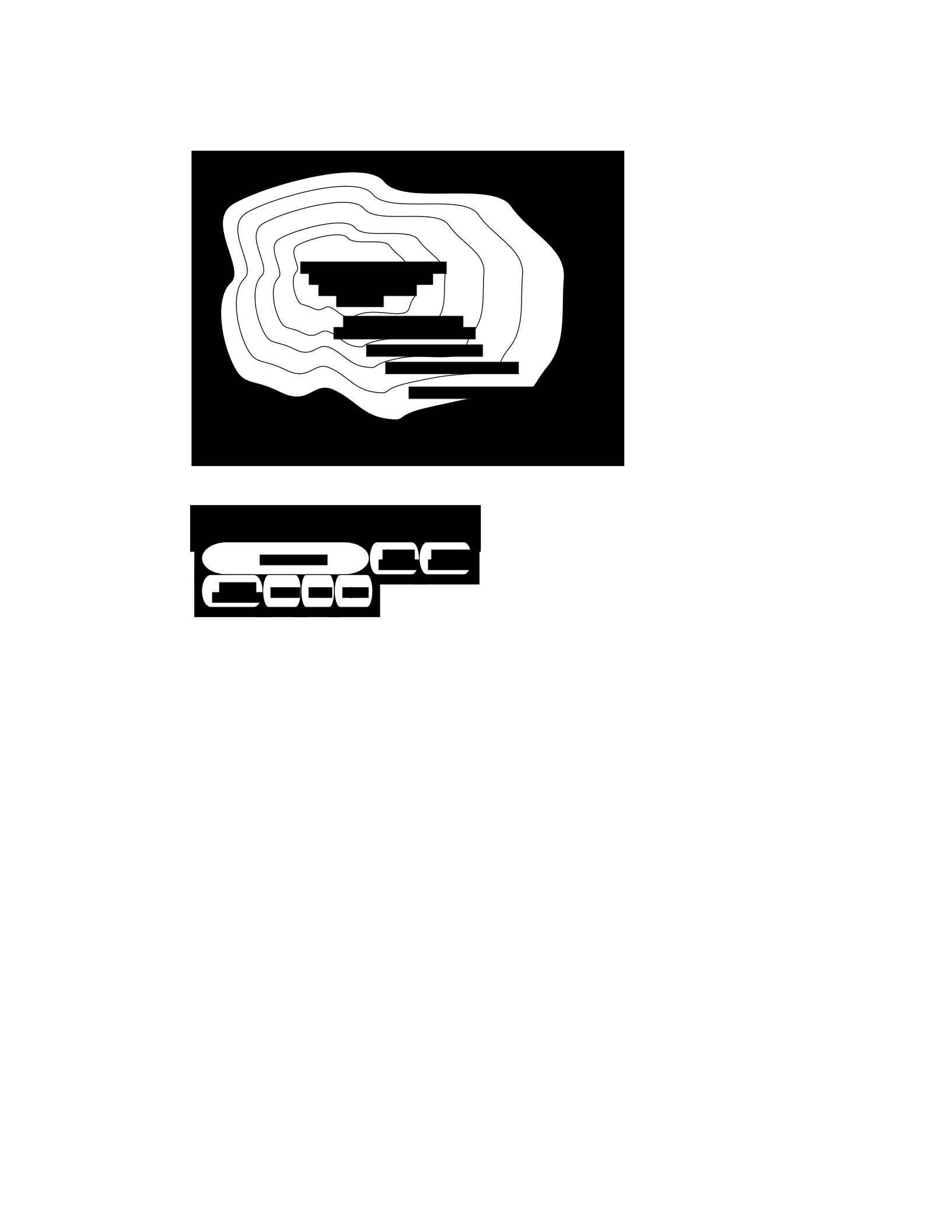
Let’s explore the abstraction hierarchy figure 1.1 in some more detail, moving up abstraction levels while
observing common patterns.
Figure 1.1 Increasingly constrained systems.
Figure 1.2 A single abstraction may have a variety of different underlying implementations.
Circuits
Typical electronics circuits are built out of a basis set of primitive components such as voltage sources,
resistors, capacitors, inductors and transistors. This set of component types was chosen to be closely
related to primitive concepts in our physical understanding of electronic systems in terms of voltage,
current, resistance, and the rate of change of those quantities over time. So, when we buy a physical
resistor, we tend to think only of its resistance; and when we buy a capacitor, we think of its ability to store
charge. But, of course, that physical resistor has some capacitance, and the capacitor, some resistance.
Still, it helps us in our designs to have devices that are as close to the ideal models as possible; and it helps
that people have been designing with these components for years, so that we can adopt the strategies
that generations of clever people have developed.
The method of combining circuit elements is to connect their terminals with conductors (wires, crimps,
solder, etc.), a process that is generically referred to as wiring. And our method of abstraction is to describe
the constraints that a circuit element exerts on the currents and voltages of terminals to which the
element is connected.
So, armed with the standard basis set of analog circuit components, we can try to build a circuit to control
our robot. We have a resistance that varies with the light level, but we need a voltage that does so, as well.
electrical systems
traditional analog circuits
digital electronic circuits
electronic computers
electronic computers
running Python programs
electronic computers with
Python programs that
select outputs by
planning
General-purpose computer
Digital circuits
T
uring
machine
Cellular
automata
Analog
electronics
Gears
Light
W
ater

wo
ep
ggg
ee
ee
ore
erg
ee
We can achieve this by using a voltage divider, which is shown in figure 1.3A. Using an abstract, constraint-
based model of the behavior of circuit components that we will

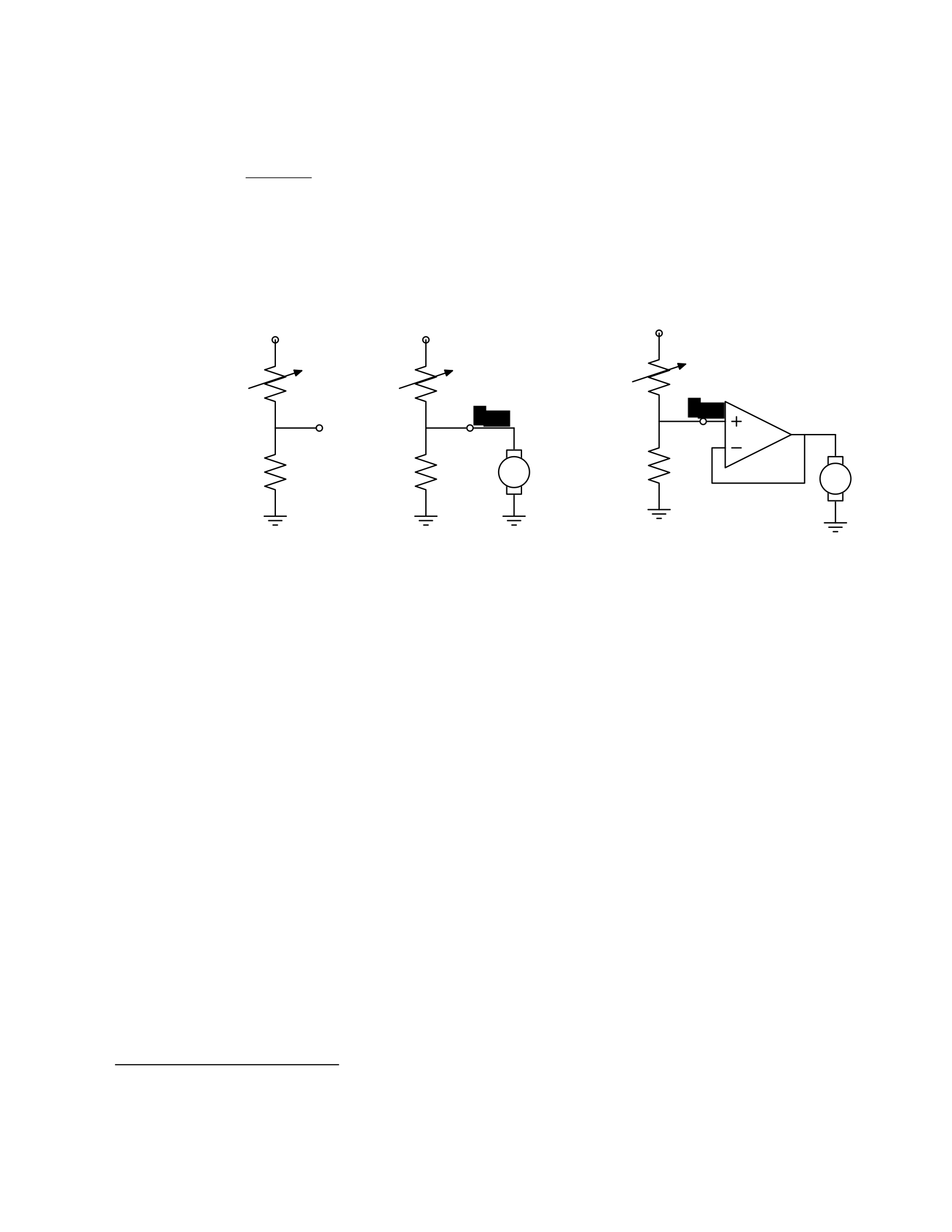
study in detail later in the course, we can determine the following relationship between Vout and
Vin:
RB
Vout = Vin .
RA + RB
So, for example, if RA = RB, then Vout = Vin/2. Or, in our case, if RA actually varies with the amount
of light shining on it, then Vout will also vary with the light.
1
Vin Vin Vin
RARARA
Vout
RBRBmotor RBmotor
Figure 1.3 Voltage dividers: A. Resistor divider. B. Connected to a motor, in a way that breaks
the abstraction from part A. C. Connected to a motor, with a buffer.
That is great. So, now, we might imagine that we could use this voltage difference that we have
created to drive the motor at different speeds, depending on the light hitting the resistor, using
a circuit something like the one shown in figure 1.3B. But, sadly, that will not work. It turns out
that once we connect the motor to the circuit, it actually changes the voltages, and we can no
longer maintain the voltage difference needed to drive the motor.
So, although we have developed an abstract model of the behavior of circuit components, which
lets us analyze the behavior of a particular complete circuit design, it does not give us
modularity. That is, we cannot design two parts of a circuit, understand each of their behaviors,
and then predict the behavior of the composite system based on the behavior of the separate
components. Instead, we would have to re-analyze the joint behavior of the whole composite
system. Lack of modularity makes it very difficult to design large systems, because two different
people, or the same person at two different times, cannot design pieces and put them together
without understanding the whole.
To solve this problem, we can augment our analog-circuit toolbox with some additional
components that allow us to design components with modular behavior; they “buffer” or
“isolate” one part of the circuit from another in ways that allow us to combine the parts more
1
Do not worry if this example does not make much sense to you; we will explore this all in great detail later.

easily. In this class, we will use op-amps to build buffers, which will let us solve our sample
problem using a slightly more complex circuit, as shown in figure 1.3C.
Thus, the key point is that good modules preserve abstraction barriers between the use of a
module and internal details of how they are constructed. We will see this theme recur as we
discuss different PCAP systems.
Digital circuits
In analog circuits, we think about voltages on terminals ranging over real values. This gives us
the freedom to create an enormous variety of circuits, but sometimes that freedom actually
makes the design process more difficult. To design ever more complex circuits, we can move to
a much stronger, digital abstraction, in which the voltages on the terminals are thought of as
only taking on values that are either “low” or “high” (often called 0 and 1). This PCAP system is
made up of a basis set of elements, called gates, that are built out of simpler analog circuit
components, such as transistors and resistors. Adopting the digital abstraction is a huge
limitation on the kinds of circuits that can be built. However, digital circuits can be easy to design
and build and also can be inexpensive because the basic elements (gates) are simple (fewer
transisters are need to construct a gate than to construct an op amp), versatile (only a small
number of different kinds of logic elements are necessary to construct an arbitrary digital
circuit), and combinations are easy to think about (using Boolean logic). These properties allow
designers to build incredibly complex machines by designing small parts and putting them
together into increasingly larger pieces. Digital watches, calculators, and computers are all built
this way.
Digital design is a very important part of EECS, and it is treated in a number of our courses at
basic and advanced levels, but is not one of the topics we will go into in detail in 6.01.
Nevertheless, the same central points that we explore in this course apply to this domain as
well.
Computers
One of the most important developments in the design of digital circuits is that of the
generalpurpose “stored program” computer. Computers are a particular class of digital circuits
that are general purpose: the same actual circuit can perform (almost) any transformation
between its inputs and its outputs. Which particular transformation it performs is governed by
a program, which is some settings of physical switches, or information written on an external
physical memory, such as cards or a tape, or information stored in some sort of internal memory.
The “almost” in the previous section refers to the actual memory capacity of the computer.
Exactly what computations a computer can perform depends on the amount of memory it has;
and also on the time you are willing to wait. So, although a general-purpose computer can do
anything a special-purpose digital circuit can do, in the information-processing sense, the
computer might be slower or use more power. However, using general-purpose computers can
save an enormous amount of engineering time and effort. It is much cheaper and easier to
debug and modify and manufacture software than hardware. The modularities and abstractions
that software PCAP systems give us are even more powerful than those derived from the digital
circuit abstraction.

Again, we can see how abstraction separates use from details; we don’t need to know how the
circuits inside a computer are designed, we just need to know the rules by which we can use
them and the constraints under which they perform.
Python programs
Every general-purpose computer has a different detailed design, which means that the way its
program needs to be specified is different. Furthermore, the “machine languages” for
describing computer programs, at the most primitive level, are awkward for human
programmers. So, we have developed a number of computer programming languages for
specifying a desired computation. These languages are converted into instructions in the
computer’s native machine language by other computer programs, called compilers or
interpreters. One of the coolest and most powerful things about general-purpose computers is
this ability to write computer programs that process or create or modify other computer
programs.
Computer programming languages are PCAP systems. They provide primitive operations, ways
of combining them, ways of abstracting over them, and ways of capturing common abstraction
patterns. We will spend a considerable amount of time in this course studying the particular
primitives, combination mechanisms, and abstraction mechanisms made available in the
Python programming language. But the choice of Python is relatively unimportant. Virtually all
modern programming languages supply a similar set of mechanisms, and the choice of
programming language is primarily a matter of taste and convenience.
In a computer program we have both data primitives and computation primitives. At the most
basic level, computers generally store binary digits (bits) in groups of 32 or 64, called words.
These words are data primitives, and they can be interpreted by our programs as representing
integers, floating-point numbers, strings, or addresses of other data in the computer’s memory.
The computational primitives supported by most computers include numerical operations such
as addition and multiplication, and locating and extracting the contents of a memory at a given
address. In Python, we will work at a level of abstraction that does not require us to think very
much about addresses of data, but it is useful to understand that level of description, as well.
Primitive data and computation elements can be combined and abstracted in a variety of
different ways, depending on choices of programming style. We will explore these in more detail
in section 1.3.2.
1.2.3 Models
So far, we have discussed a number of ways of framing the problem of designing and
constructing mechanisms. Each PCAP system is accompanied by a modeling system that lets us
make mathematical models of the systems we construct.
What is a model? It is a new system that is considerably simpler than the system being modeled,
but which captures the important aspects of the original system. We might make a physical
model of an airplane to test in a wind tunnel. It does not have to have passenger seats or landing
lights; but it has to have surfaces of the correct shape, in order to capture the important
properties for this purpose. Mathematical models can capture properties of systems that are

important to us, and allow us to discover things about the system much more conveniently than
by manipulating the original system itself.
One of the hardest things about building models is deciding which aspects of the original system
to model and which ones to ignore. Many classic, dramatic engineering failures can be ascribed
to failing to model important aspects of the system. One example (which turned out to be an
ethical success story, rather than a failure) is LeMessurier’s Citicorp Building
2
, in which an
engineering design change was made, but tested in a model in which the wind came only from
a limited set of directions.
Another important dimension in modeling is whether the model is deterministic or not. We
might, for example, model the effect of the robot executing a command to set its velocity as
making an instantaneous change to the commanded velocity. But, of course, there is likely to
be some delay and some error. We have to decide whether to ignore that delay and error in our
model and treat it as if it were ideal; or, for example, to make a probabilistic model of the
possible results of that command. Generally speaking, the more different the possible outcomes
of a particular action or command, and the more diffuse the probability distribution over those
outcomes, the more important it is to explicitly include uncertainty in the model.
Once we have a model, we can use it in a variety of different ways, which we explore below.
Analytical models
By far the most prevalent use of models is in analysis: Given a circuit design, what will the
voltage on this terminal be? Given a computer program, will it compute the desired answer?
How long will it take? Given a control system, implemented as a circuit or as a program, will the
system stop at the right distance from the light bulb?
Analytical tools are important. It can be hard to verify the correctness of a system by trying it in
all possible initial conditions with all possible inputs; sometimes it is easier to develop a
mathematical model and then prove a theorem about the model.
For some systems, such as pure software computations, or the addition circuitry in a calculator,
it is possible to analyze correctness or speed with just a model of the system in question. For
other systems, such as fuel injectors, it is impossible to analyze the correctness of the controller
without also modeling the environment (or “plant”) to which it is connected, and then analyzing
the behavior of the coupled system of the controller and environment.
To demonstrate some of these tradeoffs, we can do a very simple analysis of a robot moving
toward a lamp. Imagine that we arrange it so that the robot’s velocity at time t, V[t], is
proportional to the difference between the actual light level, X[t], and a desired light level (that
is, the light level we expect to encounter when the robot is the desired distance from the lamp),
Xdesired ; that is, we can model our control system with the difference equation
2
See “The Fifty-Nine Story Crisis”, The New Yorker, May 29, 1995, pp 45-53.

V[t] = k(Xdesired − X[t]) where k is the constant of
proportionality, or gain, of the controller.
Now, we need to model the world. For simplicity, we equate the light level to the robot’s position
(assuming that the units match); in addition we assume the robot’s position at time t is its
position at time t−1 plus its velocity at time t−1 (actually, this should be the product of the
velocity and the length of time between samples, but we can just assume a unit time step and
thus use velocity). When we couple these models, we get the difference equation
X[t] = X[t − 1] + k(Xdesired − X[t − 1]) .
Now, for a given value of k, we can determine how the system will behave over time, by solving
the difference equation in X.
Later in the course, we will see how easily-determined mathematical properties of a
differenceequation model can tell us whether a control system will have the desired behavior
and whether or not the controller will cause the system to oscillate. These same kinds of
analyses can be applied to robot control systems as well as to the temporal properties of
voltages in a circuit, and even to problems as unrelated as the consequences of a monetary
policy decision in economics. It is important to note that treating the system as moving in
discrete time steps is an approximation to underlying continuous dynamics; it can make models
that are easier to analyze, but it requires sophisticated understanding of sampling to understand
the effects of this approximation on the correctness of the results.
Synthetic models
One goal of many people in a variety of sub-disciplines of computer science and electrical
engineering is automatic synthesis of systems from formal descriptions of their desired
behavior. For example, you might describe some properties you would want the input/output
behavior of a circuit or computer program to have, and then have a computer system discover
a circuit or program with the desired property.
This is a well-specified problem, but generally the search space of possible circuits or programs
is much too large for an automated process; the intuition and previous experience of an expert
human designer cannot yet be matched by computational search methods.
However, humans use informal models of systems for synthesis. The documentation of a
software library, which describes the function of the various procedures, serves as an informal
model that a programmer can use to assemble those components to build new, complex
systems.
Internal models
As we wish to build more and more complex systems with software programs as controllers, we
find that it is often useful to build additional layers of abstraction on top of the one provided by
a generic programming language. This is particularly true when the nature of the exact

computation required depends considerably on information that is only received during the
execution of the system.
Consider, for example, an automated taxi robot (or, more prosaically, the navigation system in
your new car). It takes, as input, a current location in the city and a goal location, and gives, as
output, a path from the current location to the goal. It has a map built into it.
It is theoretically possible to build an enormous digital circuit or computer program that
contains a look-up table, in which we precompute the path for all pairs of locations and store
them away. Then when we want to find a path, we could simply look in the table at the location
corresponding to the start and goal location and retrieve the precomputed path. Unfortunately,
the size of that table is too huge to contemplate. Instead, what we do is construct an abstraction
of the problem as one of finding a path from any start state to any goal state, through a graph
(an abstract mathematical construct of “nodes” with “arcs” connecting them). We can develop
and implement a general-purpose algorithm that will solve any shortest-path problem in a
graph. That algorithm and implementation will be useful for a wide variety of possible problems.
And for the navigation system, all we have to do is represent the map as a graph, specify the
start and goal states, and call the general graph-search algorithm.
We can think of this process as actually putting a model of the system’s interactions with the
world inside the controller; it can consider different courses of action in the world and pick the
one that is the best according to some criterion.
Another example of using internal models is when the system has some significant lack of
information about the state of the environment. In such situations, it may be appropriate to
explicitly model the set of possible states of the external world and their associated
probabilities, and to update this model over time as new evidence is gathered. We will pursue
an example of this approach near the end of the course.
1.3 Programming embedded systems
There are many different ways of thinking about modularity and abstraction for software.
Different models will make some things easier to say and do and others more difficult, making
different models appropriate for different tasks. In the following sections, we explore different
strategies for building software systems that interact with an external environment, and then
different strategies for specifying the purely computational part of a system.
1.3.1 Interacting with the environment
Increasingly, computer systems need to interact with the world around them, receiving
information about the external world, and taking actions to affect the world. Furthermore, the
world is dynamic, so that as the system is computing, the world is changing, requiring future
computation to adapt to the new state of the world.
There are a variety of different ways to organize computations that interact with an external
world. Generally speaking, such a computation needs to:
1. get information from sensors (light sensors, sonars, mouse, keyboard, etc.),
2. perform computation, remembering some of the results, and

3. take actions to change the outside world (move the robot, print, draw, etc.).
These operations can be put together in different styles.
1.3.1.1 Sequential
The most immediately straightforward style for constructing a program that interacts with the
world is the basic imperative style, in which the program gives a sequence of ’commands’ to the
system it is controlling. A library of special procedures is defined, some of which read
information from the sensors and others of which cause actions to be performed. Example
procedures might move a robot forward a fixed distance, or send a file out over the network, or
move video-game characters on the screen.
In this model, we could naturally write a program that moves an idealized robot in a square, if
there is space in front of it.
if noObstacleInFront:
moveDistance(1)
turnAngle(90)
moveDistance(1)
turnAngle(90)
moveDistance(1)
turnAngle(90)
moveDistance(1)
turnAngle(90)
The major problem with this style of programming is that the programmer has to remember to
check the sensors sufficiently frequently. For instance, if the robot checks for free space in front,
and then starts moving, it might turn out that a subsequent sensor reading will show that there
is something in front of the robot, either because someone walked in front of it or because the
previous reading was erroneous. It is hard to have the discipline, as a programmer, to remember
to keep checking the sensor conditions frequently enough, and the resulting programs can be
quite difficult to read and understand.
For the robot moving toward the light, we might write a program like this:
while lightValue <
desiredValue:
moveDistance(0.1)
This would have the robot creep up, step by step, toward the light. We might want to modify it
so that the robot moved a distance that was related to the difference between the current and
desired light values. However, if it takes larger steps, then during the time that it is moving it
will not be sensitive to possible changes in the light value and cannot react immediately to
them.
1.3.1.2 Event-Driven
User-interface programs are often best organized differently, as event-driven (also called
interrupt driven) programs. In this case, the program is specified as a collection of procedures

(called ’handlers’ or ’callbacks’) that are attached to particular events that can take place. So,
for example, there might be procedures that are called when the mouse is clicked on each
button in the interface, when the user types into a text field, or when the temperature of a
reactor gets too high. An “event loop” runs continuously, checking to see whether any of the
triggering events have happened, and, if they have, calling the associated procedure.
In our simple example, we might imagine writing a program that told the robot to drive forward
by default; and then install an event handler that says that if the light level reaches the desired
value, it should stop. This program would be reactive to sudden changes in the environment.
As the number and frequency of the conditions that need responses increases, it can be difficult
to both keep a program like this running well and guarantee a minimum response time to any
event.
1.3.1.3 Transducer
An alternative view is that programming a system that interacts with an external world is like
building a transducer with internal state. Think of a transducer as a processing box that runs
continuously. At regular intervals (perhaps many times per second), the transducer reads all of
the sensors, does a small amount of computation, stores some values it will need for the next
computation, and then generates output values for the actions.
This computation happens over and over and over again. Complex behavior can arise out of the
temporal pattern of inputs and outputs. So, for example, a robot might try to move forward
without hitting something by defining a procedure:
def step(): distToFront = min(frontSonarReadings)
motorOutput(gain * (distToFront - desiredDistance), 0.0)
Executed repeatedly, this program will automatically modulate the robot’s speed to be
proportional to the free space in front of it.
The main problem with the transducer approach is that it can be difficult to do tasks that are
fundamentally sequential (like the example of driving in a square, shown above). We will start
with the transducer model, and then, as described in section 4.3, we will build a new abstraction
layer on top of it that will make it easy to do sequential commands, as well.
1.3.2 Programming models
Just as there are different strategies for organizing entire software systems, there are different
strategies for formally expressing computational processes within those structures.
1.3.2.1 Imperative computation
Most of you have probably been exposed to an imperative model of computer programming, in
which we think of programs as giving a sequential set of instructions to the computer to do
something. And, in fact, that is how the internals of the processors of computers are typically
structured. So, in Java or C or C++, you write typically procedures that consist of lists of
instructions to the computer:

1. Put this value in this variable
2. Square the variable
3. Divide it by pi
4. If the result is greater than 1, return the result
In this model of computation, the primitive computational elements are basic arithmetic
operations and assignment statements. We can combine the elements using sequences of
statements, and control structures such as if, for, and while. We can abstract away from the
details of a computation by defining a procedure that does it. Now, the engineer only needs to
know the specifications of the procedure, but not the implementation details, in order to use
it.
1.3.2.2 Functional computation
Another style of programming is the functional style. In this model, we gain power through
function calls. Rather than telling the computer to do things, we ask it questions: What is 4 + 5?
What is the square root of 6? What is the largest element of the list?
These questions can all be expressed as asking for the value of a function applied to some
arguments. But where do the functions come from? The answer is, from other functions. We
start with some set of basic functions (like “plus”), and use them to construct more complex
functions.
This method would not be powerful without the mechanisms of conditional evaluation and
recursion. Conditional functions ask one question under some conditions and another question
under other conditions. Recursion is a mechanism that lets the definition of a function refer to
the function being defined. Recursion is as powerful as iteration.
In this model of computation, the primitive computational elements are typically basic
arithmetic and list operations. We combine elements using function composition (using the
output of one function as the input to another), if, and recursion. We use function definition as
a method of abstraction, and the idea of higher-order functions (passing functions as arguments
to other functions) as a way of capturing common high-level patterns.
1.3.2.3 Data structures
In either style of asking the computer to do work for us, we have another kind of modularity
and abstraction, which is centered around the organization of data.
At the most primitive level, computers operate on collections of (usually 32 or 64) bits. We can
interpret such a collection of bits as representing different things: a positive integer, a signed
integer, a floating-point number, a Boolean value (true or false), one or more characters, or an
address of some other data in the memory of the computer. Python gives us the ability to work
directly with all of these primitives, except for addresses.
There is only so much you can do with a single number, though. We would like to build computer
programs that operate on representations of documents or maps or circuits or social networks.

To do so, we need to aggregate primitive data elements into more complex data structures.
These can include lists, arrays, dictionaries, and other structures of our own devising.
Here, again, we gain the power of abstraction. We can write programs that do operations on a
data structure representing a social network, for example, without having to worry about the
details of how the social network is represented in terms of bits in the machine.
1.3.2.4 Object-oriented programming: computation + data structures
Object-oriented programming is a style that applies the ideas of modularity and abstraction to
execution and data at the same time.
An object is a data structure, together with a set of procedures that operate on the data. Basic
procedures can be written in an imperative or a functional style, but ultimately there is
imperative assignment to state variables in the object.
One major new type of abstraction in OO programming is “generic” programming. It might be
that all objects have a procedure called print associated with them. So, we can ask any object
to print itself, without having to know how it is implemented. Or, in a graphics system, we might
have a variety of different objects that know their x,y positions on the screen. So each of them
can be asked, in the same way, to say what their position is, even though they might be
represented very differently inside the objects.
In addition, most object-oriented systems support inheritance, which is a way to make new
kinds of objects by saying that they are mostly like another kind of object, but with some
exceptions.
This is another way to take advantage of abstraction.
Programming languages
Python as well as other modern programming languages, such as Java, Ruby and C++, support
all of these programming models. The programmer needs to choose which programming model
best suits the task. This is an issue that we will return to throughout the course.
1.4 Summary
We hope that this course will give you a rich set of conceptual tools and practical techniques,
as well as an appreciation of how math, modeling, and implementation can work together to
enable the design and analysis of complex computational systems that interact with the world.
Acknowledgments
Thanks to Jacob White, Hal Abelson, Tomas Lozano-Perez, Sarah Finney, Sari Canelake, Eric
Grimson, Ike Chuang, and Berthold Horn for useful comments and criticisms, and to Denny
Freeman for significant parts and most of the figures in the linear systems chapter. - LPK
1.1 Goals for 6.01
We have many goals for this course. Our primary goal is for you to learn to appreciate and use the
fundamental design principles of modularity and abstraction in a variety of contexts from electrical

engineering and computer science. To achieve this goal, we will study electrical engineering (EE) and
computer science (CS) largely from the perspective of how to build systems that interact with, and attempt
to control, an external environment. Such systems include everything from low-level controllers like heat
regulators or cardiac pacemakers, to medium-level systems like automated navigation or virtual surgery,
to high-level systems that provide more natural human-computer interfaces.
Our second goal is to show you that making mathematical models of real systems can help in the design
and analysis of those systems; and to give you practice with the difficult step of deciding which aspects of
the real world are important to the problem being solved and how to model them in ways that give insight
into the problem.
We also hope to engage you more actively in the educational process. Most of the work of this course will
not be like typical problems from the end of a chapter. You will work individually and in pairs to solve
problems that are deeper and more open-ended. There will not be a unique right answer. Argument,
explanation, and justification of approach will be more important than the answer. We hope to expose
you to the ubiquity of trade-offs in engineering design: it is rare that an approach will be best in every
dimension; some will excel in one way, others in a different way. Deciding how to make such trade-offs is
a crucial part of engineering.
Another way in which we hope to engage you in the material is by having many of you return to the course
as lab assistants in future semesters. Having a large number of lab assistants in the class means that
students can be given more open-ended problems, and have people around to help them when they are
stuck. Even more importantly, the lab assistants are meant to question the students as they go; to
challenge their understanding and help them see and evaluate a variety of approaches. This process is of
great intellectual value to student and lab assistant alike.
Finally, of course, we have the more typical goals of teaching exciting and important basic material from
electrical engineering and computer science, including modern software engineering, linear systems
analysis, electronic circuits, and decision-making. This material all has an internal elegance and beauty, as
well as crucial role in building modern EE and CS systems.
1.2 Modularity, abstraction, and modeling
Whether proving a theorem by building up from lemmas to basic theorems to more specialized results, or
designing a circuit by building up from components to modules to complex processors, or designing a
software system by building up from generic procedures to classes to class libraries, humans deal with
complexity by exploiting the power of abstraction and modularity. Without such tools, a single person
would be overwhelmed by the complexity of a system, as there is only so much detail that a single person
can consciously manage at a time.
Modularity is the idea of building components that can be re-used; and abstraction is the idea that after
constructing a module (be it software or circuits or gears), most of the details of the module construction
can be ignored and a simpler description used for module interaction (the module computes the square
root, or doubles the voltage, or changes the direction of motion).
Given basic modules, one can move up a level of abstraction and construct a new module by putting
together several previously-built modules, thinking only of their abstract descriptions, and not their
implementations. And, of course, this process can be repeated over many stages. This process gives one

the ability to construct systems with complexity far beyond what would be possible if it were necessary to
understand each component in detail.
Any module can be described in a large number of ways. We might describe the circuitry in a digital watch
in terms of how it behaves as a clock and a stopwatch, or in terms of voltages and currents within the
circuit, or in terms of the heat produced at different parts of the circuitry. Each of these is a different model
of the watch. Different models will be appropriate for different tasks: there is no single correct model.
Rather, each model exposes different dimensions of the system, allowing us to explore many aspects of
the design space of a system, and to trade off different factors in the performance of a system.
The primary theme of this course will be to learn about different methods for building modules out of
primitives, and of building different abstract models of them, so that we can analyze or predict their
behavior, and so we can recombine them into even more complex systems. The same fundamental
principles will apply to software, to control systems, and to circuits.
1.2.1 Example problem
Imagine that you need to make a robot that will roll up close to a light bulb and stop a fixed distance from
it. The first question is, how can we get electrical signals to relate to the physical phenomena of light
readings and robot wheel rotations? There is a large part of electrical engineering related to the design of
physical devices that connect to the physical world in such a way that some electrical property of the
device relates to a physical process in the world. For example, a light-sensitive resistor (photo-resistor) is
a sensor whose resistance changes depending on light intensity impinging on it; a motor is an effector
whose rotor speed is related to the voltage across its two terminals. In this course, we will not examine
the detailed physics of sensors and effectors, but will concentrate on ways of designing systems that use
sensors and effectors to perform both simple and more complicated tasks. To get a robot to stop in front
of a light bulb, the problem will be to find a way to connect the photo-resistor to the motor, so that the
robot will stop at an appropriate distance from the bulb. Thus, we will already use the idea of abstraction
to treat sensors Chapter 1 Course Overview
and effectors as primitive modules whose internal details we can ignore, and whose performance
characteristics we can use as we design systems built on these elements.
1.2.2 An abstraction hierarchy of mechanisms
Given the light-sensitive resistor and the motor, we could find many ways of connecting them, using bits
of metal and ceramic of different kinds, or making some kind of magnetic or mechanical linkages. The
space of possible designs of machines is enormous.
One of the most important things that engineers do, when faced with a set of design problems, is to
standardize on a basis set of components to use to build their systems. There are many reasons for
standardizing on a basis set of components, mostly having to do with efficiency of understanding and of
manufacturing. It is important, as a designer, to develop a repertoire of standard bits and pieces of designs
that you understand well and can put together in various ways to make more complex systems. If you use
the same basis set of components as other designers, you can learn valuable techniques from them, rather
than having to re-invent the techniques yourself. And other people will be able to readily understand and
modify your designs.
We can often make a design job easier by limiting the space of possible designs, and by standardizing on:
• a basis set of primitive components;
• ways of combining the primitive components to make more complex systems;
• ways of “packaging” or abstracting pieces of a design so they can be reused (in essence creating
new “primitives”); and
• ways of capturing common patterns of abstraction (essentially, abstracting our abstractions).
Very complicated design problems can become tractable using such a primitive-combinationabstraction-
pattern (PCAP) approach. In this class, we will examine and learn to use a variety of PCAP strategies
common in EE and CS, and will even design some of our own, for special purposes. In the rest of this
section, we will hint at some of the PCAP systems we will be developing in much greater depth throughout
the class. Figure 1.1 shows one view of this development, as a successive set of restrictions of the design
space of mechanisms.
One very important thing about abstract models is that once we have fixed the abstraction, it will usually
be possible to implement it using a variety of different underlying substrates. So, as shown in figure 1.2,
we can construct general-purpose computers out of a variety of different kinds of systems, including digital
circuits and general-purpose computers. And systems satisfying the digital circuit abstraction can be
constructed from analog circuits, but also from gears or water or light.
Another demonstration of the value of abstracted models is that we can use them, by analogy, to describe
quite different systems. So, for example, the constraint models of circuits that we will study can be applied
to describing transmission of neural signals down the spinal cord, or of heat through a network of
connected bodies.
Let’s explore the abstraction hierarchy figure 1.1 in some more detail, moving up abstraction levels while
observing common patterns.
Figure 1.1 Increasingly constrained systems.
electrical systems
traditional analog circuits
digital electronic circuits
electronic computers
electronic computers
running Python programs
electronic computers with
Python programs that
select outputs by
planning

Figure 1.2 A single abstraction may have a variety of different underlying implementations.
Circuits
Typical electronics circuits are built out of a basis set of primitive components such as voltage sources,
resistors, capacitors, inductors and transistors. This set of component types was chosen to be closely
related to primitive concepts in our physical understanding of electronic systems in terms of voltage,
current, resistance, and the rate of change of those quantities over time. So, when we buy a physical
resistor, we tend to think only of its resistance; and when we buy a capacitor, we think of its ability to store
charge. But, of course, that physical resistor has some capacitance, and the capacitor, some resistance.
Still, it helps us in our designs to have devices that are as close to the ideal models as possible; and it helps
that people have been designing with these components for years, so that we can adopt the strategies
that generations of clever people have developed.
The method of combining circuit elements is to connect their terminals with conductors (wires, crimps,
solder, etc.), a process that is generically referred to as wiring. And our method of abstraction is to describe
the constraints that a circuit element exerts on the currents and voltages of terminals to which the
element is connected.
So, armed with the standard basis set of analog circuit components, we can try to build a circuit to control
our robot. We have a resistance that varies with the light level, but we need a voltage that does so, as well.
We can achieve this by using a voltage divider, which is shown in figure 1.3A. Using an abstract, constraint-
based model of the behavior of circuit components that we will
General-purpose computer
Digital circuits
T
uring
machine
Cellular
automata
Analog
electronics
Gears
Light
W
ater
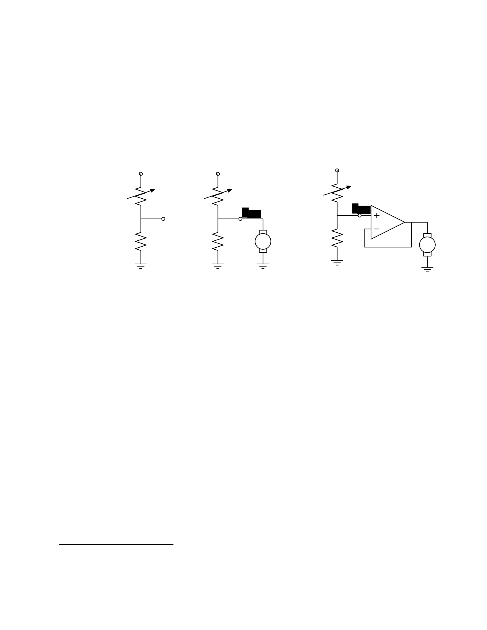
study in detail later in the course, we can determine the following relationship between Vout and
Vin:
RB
Vout = Vin .
RA + RB
So, for example, if RA = RB, then Vout = Vin/2. Or, in our case, if RA actually varies with the amount
of light shining on it, then Vout will also vary with the light.
3
Vin Vin Vin
RARARA
Vout
RBRBmotor RBmotor
Figure 1.3 Voltage dividers: A. Resistor divider. B. Connected to a motor, in a way that breaks
the abstraction from part A. C. Connected to a motor, with a buffer.
That is great. So, now, we might imagine that we could use this voltage difference that we have
created to drive the motor at different speeds, depending on the light hitting the resistor, using
a circuit something like the one shown in figure 1.3B. But, sadly, that will not work. It turns out
that once we connect the motor to the circuit, it actually changes the voltages, and we can no
longer maintain the voltage difference needed to drive the motor.
So, although we have developed an abstract model of the behavior of circuit components, which
lets us analyze the behavior of a particular complete circuit design, it does not give us
modularity. That is, we cannot design two parts of a circuit, understand each of their behaviors,
and then predict the behavior of the composite system based on the behavior of the separate
components. Instead, we would have to re-analyze the joint behavior of the whole composite
system. Lack of modularity makes it very difficult to design large systems, because two different
people, or the same person at two different times, cannot design pieces and put them together
without understanding the whole.
To solve this problem, we can augment our analog-circuit toolbox with some additional
components that allow us to design components with modular behavior; they “buffer” or
“isolate” one part of the circuit from another in ways that allow us to combine the parts more
3
Do not worry if this example does not make much sense to you; we will explore this all in great detail later.

easily. In this class, we will use op-amps to build buffers, which will let us solve our sample
problem using a slightly more complex circuit, as shown in figure 1.3C.
Thus, the key point is that good modules preserve abstraction barriers between the use of a
module and internal details of how they are constructed. We will see this theme recur as we
discuss different PCAP systems.
Digital circuits
In analog circuits, we think about voltages on terminals ranging over real values. This gives us
the freedom to create an enormous variety of circuits, but sometimes that freedom actually
makes the design process more difficult. To design ever more complex circuits, we can move to
a much stronger, digital abstraction, in which the voltages on the terminals are thought of as
only taking on values that are either “low” or “high” (often called 0 and 1). This PCAP system is
made up of a basis set of elements, called gates, that are built out of simpler analog circuit
components, such as transistors and resistors. Adopting the digital abstraction is a huge
limitation on the kinds of circuits that can be built. However, digital circuits can be easy to design
and build and also can be inexpensive because the basic elements (gates) are simple (fewer
transisters are need to construct a gate than to construct an op amp), versatile (only a small
number of different kinds of logic elements are necessary to construct an arbitrary digital
circuit), and combinations are easy to think about (using Boolean logic). These properties allow
designers to build incredibly complex machines by designing small parts and putting them
together into increasingly larger pieces. Digital watches, calculators, and computers are all built
this way.
Digital design is a very important part of EECS, and it is treated in a number of our courses at
basic and advanced levels, but is not one of the topics we will go into in detail in 6.01.
Nevertheless, the same central points that we explore in this course apply to this domain as
well.
Computers
One of the most important developments in the design of digital circuits is that of the
generalpurpose “stored program” computer. Computers are a particular class of digital circuits
that are general purpose: the same actual circuit can perform (almost) any transformation
between its inputs and its outputs. Which particular transformation it performs is governed by
a program, which is some settings of physical switches, or information written on an external
physical memory, such as cards or a tape, or information stored in some sort of internal memory.
The “almost” in the previous section refers to the actual memory capacity of the computer.
Exactly what computations a computer can perform depends on the amount of memory it has;
and also on the time you are willing to wait. So, although a general-purpose computer can do
anything a special-purpose digital circuit can do, in the information-processing sense, the
computer might be slower or use more power. However, using general-purpose computers can
save an enormous amount of engineering time and effort. It is much cheaper and easier to
debug and modify and manufacture software than hardware. The modularities and abstractions
that software PCAP systems give us are even more powerful than those derived from the digital
circuit abstraction.

Again, we can see how abstraction separates use from details; we don’t need to know how the
circuits inside a computer are designed, we just need to know the rules by which we can use
them and the constraints under which they perform.
Python programs
Every general-purpose computer has a different detailed design, which means that the way its
program needs to be specified is different. Furthermore, the “machine languages” for
describing computer programs, at the most primitive level, are awkward for human
programmers. So, we have developed a number of computer programming languages for
specifying a desired computation. These languages are converted into instructions in the
computer’s native machine language by other computer programs, called compilers or
interpreters. One of the coolest and most powerful things about general-purpose computers is
this ability to write computer programs that process or create or modify other computer
programs.
Computer programming languages are PCAP systems. They provide primitive operations, ways
of combining them, ways of abstracting over them, and ways of capturing common abstraction
patterns. We will spend a considerable amount of time in this course studying the particular
primitives, combination mechanisms, and abstraction mechanisms made available in the
Python programming language. But the choice of Python is relatively unimportant. Virtually all
modern programming languages supply a similar set of mechanisms, and the choice of
programming language is primarily a matter of taste and convenience.
In a computer program we have both data primitives and computation primitives. At the most
basic level, computers generally store binary digits (bits) in groups of 32 or 64, called words.
These words are data primitives, and they can be interpreted by our programs as representing
integers, floating-point numbers, strings, or addresses of other data in the computer’s memory.
The computational primitives supported by most computers include numerical operations such
as addition and multiplication, and locating and extracting the contents of a memory at a given
address. In Python, we will work at a level of abstraction that does not require us to think very
much about addresses of data, but it is useful to understand that level of description, as well.
Primitive data and computation elements can be combined and abstracted in a variety of
different ways, depending on choices of programming style. We will explore these in more detail
in section 1.3.2.
1.2.3 Models
So far, we have discussed a number of ways of framing the problem of designing and
constructing mechanisms. Each PCAP system is accompanied by a modeling system that lets us
make mathematical models of the systems we construct.
What is a model? It is a new system that is considerably simpler than the system being modeled,
but which captures the important aspects of the original system. We might make a physical
model of an airplane to test in a wind tunnel. It does not have to have passenger seats or landing
lights; but it has to have surfaces of the correct shape, in order to capture the important
properties for this purpose. Mathematical models can capture properties of systems that are

important to us, and allow us to discover things about the system much more conveniently than
by manipulating the original system itself.
One of the hardest things about building models is deciding which aspects of the original system
to model and which ones to ignore. Many classic, dramatic engineering failures can be ascribed
to failing to model important aspects of the system. One example (which turned out to be an
ethical success story, rather than a failure) is LeMessurier’s Citicorp Building
4
, in which an
engineering design change was made, but tested in a model in which the wind came only from
a limited set of directions.
Another important dimension in modeling is whether the model is deterministic or not. We
might, for example, model the effect of the robot executing a command to set its velocity as
making an instantaneous change to the commanded velocity. But, of course, there is likely to
be some delay and some error. We have to decide whether to ignore that delay and error in our
model and treat it as if it were ideal; or, for example, to make a probabilistic model of the
possible results of that command. Generally speaking, the more different the possible outcomes
of a particular action or command, and the more diffuse the probability distribution over those
outcomes, the more important it is to explicitly include uncertainty in the model.
Once we have a model, we can use it in a variety of different ways, which we explore below.
Analytical models
By far the most prevalent use of models is in analysis: Given a circuit design, what will the
voltage on this terminal be? Given a computer program, will it compute the desired answer?
How long will it take? Given a control system, implemented as a circuit or as a program, will the
system stop at the right distance from the light bulb?
Analytical tools are important. It can be hard to verify the correctness of a system by trying it in
all possible initial conditions with all possible inputs; sometimes it is easier to develop a
mathematical model and then prove a theorem about the model.
For some systems, such as pure software computations, or the addition circuitry in a calculator,
it is possible to analyze correctness or speed with just a model of the system in question. For
other systems, such as fuel injectors, it is impossible to analyze the correctness of the controller
without also modeling the environment (or “plant”) to which it is connected, and then analyzing
the behavior of the coupled system of the controller and environment.
To demonstrate some of these tradeoffs, we can do a very simple analysis of a robot moving
toward a lamp. Imagine that we arrange it so that the robot’s velocity at time t, V[t], is
proportional to the difference between the actual light level, X[t], and a desired light level (that
is, the light level we expect to encounter when the robot is the desired distance from the lamp),
Xdesired ; that is, we can model our control system with the difference equation
4
See “The Fifty-Nine Story Crisis”, The New Yorker, May 29, 1995, pp 45-53.

V[t] = k(Xdesired − X[t]) where k is the constant of
proportionality, or gain, of the controller.
Now, we need to model the world. For simplicity, we equate the light level to the robot’s position
(assuming that the units match); in addition we assume the robot’s position at time t is its
position at time t−1 plus its velocity at time t−1 (actually, this should be the product of the
velocity and the length of time between samples, but we can just assume a unit time step and
thus use velocity). When we couple these models, we get the difference equation
X[t] = X[t − 1] + k(Xdesired − X[t − 1]) .
Now, for a given value of k, we can determine how the system will behave over time, by solving
the difference equation in X.
Later in the course, we will see how easily-determined mathematical properties of a
differenceequation model can tell us whether a control system will have the desired behavior
and whether or not the controller will cause the system to oscillate. These same kinds of
analyses can be applied to robot control systems as well as to the temporal properties of
voltages in a circuit, and even to problems as unrelated as the consequences of a monetary
policy decision in economics. It is important to note that treating the system as moving in
discrete time steps is an approximation to underlying continuous dynamics; it can make models
that are easier to analyze, but it requires sophisticated understanding of sampling to understand
the effects of this approximation on the correctness of the results.
Synthetic models
One goal of many people in a variety of sub-disciplines of computer science and electrical
engineering is automatic synthesis of systems from formal descriptions of their desired
behavior. For example, you might describe some properties you would want the input/output
behavior of a circuit or computer program to have, and then have a computer system discover
a circuit or program with the desired property.
This is a well-specified problem, but generally the search space of possible circuits or programs
is much too large for an automated process; the intuition and previous experience of an expert
human designer cannot yet be matched by computational search methods.
However, humans use informal models of systems for synthesis. The documentation of a
software library, which describes the function of the various procedures, serves as an informal
model that a programmer can use to assemble those components to build new, complex
systems.
Internal models
As we wish to build more and more complex systems with software programs as controllers, we
find that it is often useful to build additional layers of abstraction on top of the one provided by
a generic programming language. This is particularly true when the nature of the exact

computation required depends considerably on information that is only received during the
execution of the system.
Consider, for example, an automated taxi robot (or, more prosaically, the navigation system in
your new car). It takes, as input, a current location in the city and a goal location, and gives, as
output, a path from the current location to the goal. It has a map built into it.
It is theoretically possible to build an enormous digital circuit or computer program that
contains a look-up table, in which we precompute the path for all pairs of locations and store
them away. Then when we want to find a path, we could simply look in the table at the location
corresponding to the start and goal location and retrieve the precomputed path. Unfortunately,
the size of that table is too huge to contemplate. Instead, what we do is construct an abstraction
of the problem as one of finding a path from any start state to any goal state, through a graph
(an abstract mathematical construct of “nodes” with “arcs” connecting them). We can develop
and implement a general-purpose algorithm that will solve any shortest-path problem in a
graph. That algorithm and implementation will be useful for a wide variety of possible problems.
And for the navigation system, all we have to do is represent the map as a graph, specify the
start and goal states, and call the general graph-search algorithm.
We can think of this process as actually putting a model of the system’s interactions with the
world inside the controller; it can consider different courses of action in the world and pick the
one that is the best according to some criterion.
Another example of using internal models is when the system has some significant lack of
information about the state of the environment. In such situations, it may be appropriate to
explicitly model the set of possible states of the external world and their associated
probabilities, and to update this model over time as new evidence is gathered. We will pursue
an example of this approach near the end of the course.
1.3 Programming embedded systems
There are many different ways of thinking about modularity and abstraction for software.
Different models will make some things easier to say and do and others more difficult, making
different models appropriate for different tasks. In the following sections, we explore different
strategies for building software systems that interact with an external environment, and then
different strategies for specifying the purely computational part of a system.
1.3.1 Interacting with the environment
Increasingly, computer systems need to interact with the world around them, receiving
information about the external world, and taking actions to affect the world. Furthermore, the
world is dynamic, so that as the system is computing, the world is changing, requiring future
computation to adapt to the new state of the world.
There are a variety of different ways to organize computations that interact with an external
world. Generally speaking, such a computation needs to:
4. get information from sensors (light sensors, sonars, mouse, keyboard, etc.),
5. perform computation, remembering some of the results, and

6. take actions to change the outside world (move the robot, print, draw, etc.).
These operations can be put together in different styles.
1.3.1.1 Sequential
The most immediately straightforward style for constructing a program that interacts with the
world is the basic imperative style, in which the program gives a sequence of ’commands’ to the
system it is controlling. A library of special procedures is defined, some of which read
information from the sensors and others of which cause actions to be performed. Example
procedures might move a robot forward a fixed distance, or send a file out over the network, or
move video-game characters on the screen.
In this model, we could naturally write a program that moves an idealized robot in a square, if
there is space in front of it.
if noObstacleInFront:
moveDistance(1)
turnAngle(90)
moveDistance(1)
turnAngle(90)
moveDistance(1)
turnAngle(90)
moveDistance(1)
turnAngle(90)
The major problem with this style of programming is that the programmer has to remember to
check the sensors sufficiently frequently. For instance, if the robot checks for free space in front,
and then starts moving, it might turn out that a subsequent sensor reading will show that there
is something in front of the robot, either because someone walked in front of it or because the
previous reading was erroneous. It is hard to have the discipline, as a programmer, to remember
to keep checking the sensor conditions frequently enough, and the resulting programs can be
quite difficult to read and understand.
For the robot moving toward the light, we might write a program like this:
while lightValue <
desiredValue:
moveDistance(0.1)
This would have the robot creep up, step by step, toward the light. We might want to modify it
so that the robot moved a distance that was related to the difference between the current and
desired light values. However, if it takes larger steps, then during the time that it is moving it
will not be sensitive to possible changes in the light value and cannot react immediately to
them.
1.3.1.2 Event-Driven
User-interface programs are often best organized differently, as event-driven (also called
interrupt driven) programs. In this case, the program is specified as a collection of procedures

(called ’handlers’ or ’callbacks’) that are attached to particular events that can take place. So,
for example, there might be procedures that are called when the mouse is clicked on each
button in the interface, when the user types into a text field, or when the temperature of a
reactor gets too high. An “event loop” runs continuously, checking to see whether any of the
triggering events have happened, and, if they have, calling the associated procedure.
In our simple example, we might imagine writing a program that told the robot to drive forward
by default; and then install an event handler that says that if the light level reaches the desired
value, it should stop. This program would be reactive to sudden changes in the environment.
As the number and frequency of the conditions that need responses increases, it can be difficult
to both keep a program like this running well and guarantee a minimum response time to any
event.
1.3.1.3 Transducer
An alternative view is that programming a system that interacts with an external world is like
building a transducer with internal state. Think of a transducer as a processing box that runs
continuously. At regular intervals (perhaps many times per second), the transducer reads all of
the sensors, does a small amount of computation, stores some values it will need for the next
computation, and then generates output values for the actions.
This computation happens over and over and over again. Complex behavior can arise out of the
temporal pattern of inputs and outputs. So, for example, a robot might try to move forward
without hitting something by defining a procedure:
def step(): distToFront = min(frontSonarReadings)
motorOutput(gain * (distToFront - desiredDistance), 0.0)
Executed repeatedly, this program will automatically modulate the robot’s speed to be
proportional to the free space in front of it.
The main problem with the transducer approach is that it can be difficult to do tasks that are
fundamentally sequential (like the example of driving in a square, shown above). We will start
with the transducer model, and then, as described in section 4.3, we will build a new abstraction
layer on top of it that will make it easy to do sequential commands, as well.
1.3.2 Programming models
Just as there are different strategies for organizing entire software systems, there are different
strategies for formally expressing computational processes within those structures.
1.3.2.1 Imperative computation
Most of you have probably been exposed to an imperative model of computer programming, in
which we think of programs as giving a sequential set of instructions to the computer to do
something. And, in fact, that is how the internals of the processors of computers are typically
structured. So, in Java or C or C++, you write typically procedures that consist of lists of
instructions to the computer:

5. Put this value in this variable
6. Square the variable
7. Divide it by pi
8. If the result is greater than 1, return the result
In this model of computation, the primitive computational elements are basic arithmetic
operations and assignment statements. We can combine the elements using sequences of
statements, and control structures such as if, for, and while. We can abstract away from the
details of a computation by defining a procedure that does it. Now, the engineer only needs to
know the specifications of the procedure, but not the implementation details, in order to use
it.
1.3.2.2 Functional computation
Another style of programming is the functional style. In this model, we gain power through
function calls. Rather than telling the computer to do things, we ask it questions: What is 4 + 5?
What is the square root of 6? What is the largest element of the list?
These questions can all be expressed as asking for the value of a function applied to some
arguments. But where do the functions come from? The answer is, from other functions. We
start with some set of basic functions (like “plus”), and use them to construct more complex
functions.
This method would not be powerful without the mechanisms of conditional evaluation and
recursion. Conditional functions ask one question under some conditions and another question
under other conditions. Recursion is a mechanism that lets the definition of a function refer to
the function being defined. Recursion is as powerful as iteration.
In this model of computation, the primitive computational elements are typically basic
arithmetic and list operations. We combine elements using function composition (using the
output of one function as the input to another), if, and recursion. We use function definition as
a method of abstraction, and the idea of higher-order functions (passing functions as arguments
to other functions) as a way of capturing common high-level patterns.
1.3.2.3 Data structures
In either style of asking the computer to do work for us, we have another kind of modularity
and abstraction, which is centered around the organization of data.
At the most primitive level, computers operate on collections of (usually 32 or 64) bits. We can
interpret such a collection of bits as representing different things: a positive integer, a signed
integer, a floating-point number, a Boolean value (true or false), one or more characters, or an
address of some other data in the memory of the computer. Python gives us the ability to work
directly with all of these primitives, except for addresses.
There is only so much you can do with a single number, though. We would like to build computer
programs that operate on representations of documents or maps or circuits or social networks.

To do so, we need to aggregate primitive data elements into more complex data structures.
These can include lists, arrays, dictionaries, and other structures of our own devising.
Here, again, we gain the power of abstraction. We can write programs that do operations on a
data structure representing a social network, for example, without having to worry about the
details of how the social network is represented in terms of bits in the machine.
1.3.2.4 Object-oriented programming: computation + data structures
Object-oriented programming is a style that applies the ideas of modularity and abstraction to
execution and data at the same time.
An object is a data structure, together with a set of procedures that operate on the data. Basic
procedures can be written in an imperative or a functional style, but ultimately there is
imperative assignment to state variables in the object.
One major new type of abstraction in OO programming is “generic” programming. It might be
that all objects have a procedure called print associated with them. So, we can ask any object
to print itself, without having to know how it is implemented. Or, in a graphics system, we might
have a variety of different objects that know their x,y positions on the screen. So each of them
can be asked, in the same way, to say what their position is, even though they might be
represented very differently inside the objects.
In addition, most object-oriented systems support inheritance, which is a way to make new
kinds of objects by saying that they are mostly like another kind of object, but with some
exceptions.
This is another way to take advantage of abstraction.
Programming languages
Python as well as other modern programming languages, such as Java, Ruby and C++, support
all of these programming models. The programmer needs to choose which programming model
best suits the task. This is an issue that we will return to throughout the course.
1.4 Summary
We hope that this course will give you a rich set of conceptual tools and practical techniques,
as well as an appreciation of how math, modeling, and implementation can work together to
enable the design and analysis of complex computational systems that interact with the world.
Acknowledgments
Thanks to Jacob White, Hal Abelson, Tomas Lozano-Perez, Sarah Finney, Sari Canelake, Eric
Grimson, Ike Chuang, and Berthold Horn for useful comments and criticisms, and to Denny
Freeman for significant parts and most of the figures in the linear systems chapter. - LPK
1.1 Goals for 6.01
We have many goals for this course. Our primary goal is for you to learn to appreciate and use the
fundamental design principles of modularity and abstraction in a variety of contexts from electrical

engineering and computer science. To achieve this goal, we will study electrical engineering (EE) and
computer science (CS) largely from the perspective of how to build systems that interact with, and attempt
to control, an external environment. Such systems include everything from low-level controllers like heat
regulators or cardiac pacemakers, to medium-level systems like automated navigation or virtual surgery,
to high-level systems that provide more natural human-computer interfaces.
Our second goal is to show you that making mathematical models of real systems can help in the design
and analysis of those systems; and to give you practice with the difficult step of deciding which aspects of
the real world are important to the problem being solved and how to model them in ways that give insight
into the problem.
We also hope to engage you more actively in the educational process. Most of the work of this course will
not be like typical problems from the end of a chapter. You will work individually and in pairs to solve
problems that are deeper and more open-ended. There will not be a unique right answer. Argument,
explanation, and justification of approach will be more important than the answer. We hope to expose
you to the ubiquity of trade-offs in engineering design: it is rare that an approach will be best in every
dimension; some will excel in one way, others in a different way. Deciding how to make such trade-offs is
a crucial part of engineering.
Another way in which we hope to engage you in the material is by having many of you return to the course
as lab assistants in future semesters. Having a large number of lab assistants in the class means that
students can be given more open-ended problems, and have people around to help them when they are
stuck. Even more importantly, the lab assistants are meant to question the students as they go; to
challenge their understanding and help them see and evaluate a variety of approaches. This process is of
great intellectual value to student and lab assistant alike.
Finally, of course, we have the more typical goals of teaching exciting and important basic material from
electrical engineering and computer science, including modern software engineering, linear systems
analysis, electronic circuits, and decision-making. This material all has an internal elegance and beauty, as
well as crucial role in building modern EE and CS systems.
1.2 Modularity, abstraction, and modeling
Whether proving a theorem by building up from lemmas to basic theorems to more specialized results, or
designing a circuit by building up from components to modules to complex processors, or designing a
software system by building up from generic procedures to classes to class libraries, humans deal with
complexity by exploiting the power of abstraction and modularity. Without such tools, a single person
would be overwhelmed by the complexity of a system, as there is only so much detail that a single person
can consciously manage at a time.
Modularity is the idea of building components that can be re-used; and abstraction is the idea that after
constructing a module (be it software or circuits or gears), most of the details of the module construction
can be ignored and a simpler description used for module interaction (the module computes the square
root, or doubles the voltage, or changes the direction of motion).
Given basic modules, one can move up a level of abstraction and construct a new module by putting
together several previously-built modules, thinking only of their abstract descriptions, and not their
implementations. And, of course, this process can be repeated over many stages. This process gives one

the ability to construct systems with complexity far beyond what would be possible if it were necessary to
understand each component in detail.
Any module can be described in a large number of ways. We might describe the circuitry in a digital watch
in terms of how it behaves as a clock and a stopwatch, or in terms of voltages and currents within the
circuit, or in terms of the heat produced at different parts of the circuitry. Each of these is a different model
of the watch. Different models will be appropriate for different tasks: there is no single correct model.
Rather, each model exposes different dimensions of the system, allowing us to explore many aspects of
the design space of a system, and to trade off different factors in the performance of a system.
The primary theme of this course will be to learn about different methods for building modules out of
primitives, and of building different abstract models of them, so that we can analyze or predict their
behavior, and so we can recombine them into even more complex systems. The same fundamental
principles will apply to software, to control systems, and to circuits.
1.2.1 Example problem
Imagine that you need to make a robot that will roll up close to a light bulb and stop a fixed distance from
it. The first question is, how can we get electrical signals to relate to the physical phenomena of light
readings and robot wheel rotations? There is a large part of electrical engineering related to the design of
physical devices that connect to the physical world in such a way that some electrical property of the
device relates to a physical process in the world. For example, a light-sensitive resistor (photo-resistor) is
a sensor whose resistance changes depending on light intensity impinging on it; a motor is an effector
whose rotor speed is related to the voltage across its two terminals. In this course, we will not examine
the detailed physics of sensors and effectors, but will concentrate on ways of designing systems that use
sensors and effectors to perform both simple and more complicated tasks. To get a robot to stop in front
of a light bulb, the problem will be to find a way to connect the photo-resistor to the motor, so that the
robot will stop at an appropriate distance from the bulb. Thus, we will already use the idea of abstraction
to treat sensors Chapter 1 Course Overview
and effectors as primitive modules whose internal details we can ignore, and whose performance
characteristics we can use as we design systems built on these elements.
1.2.2 An abstraction hierarchy of mechanisms
Given the light-sensitive resistor and the motor, we could find many ways of connecting them, using bits
of metal and ceramic of different kinds, or making some kind of magnetic or mechanical linkages. The
space of possible designs of machines is enormous.
One of the most important things that engineers do, when faced with a set of design problems, is to
standardize on a basis set of components to use to build their systems. There are many reasons for
standardizing on a basis set of components, mostly having to do with efficiency of understanding and of
manufacturing. It is important, as a designer, to develop a repertoire of standard bits and pieces of designs
that you understand well and can put together in various ways to make more complex systems. If you use
the same basis set of components as other designers, you can learn valuable techniques from them, rather
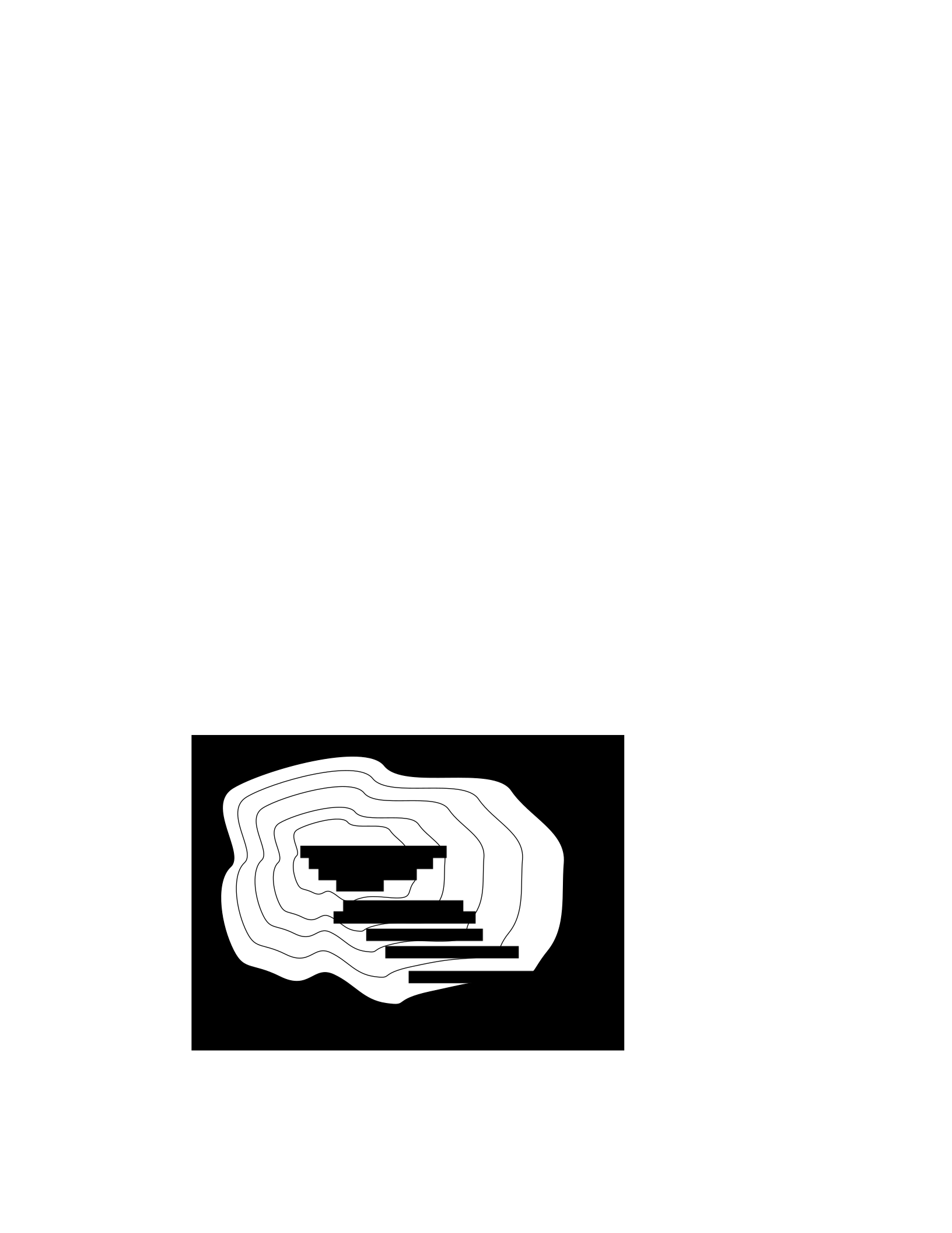
than having to re-invent the techniques yourself. And other people will be able to readily understand and
modify your designs.
We can often make a design job easier by limiting the space of possible designs, and by standardizing on:
• a basis set of primitive components;
• ways of combining the primitive components to make more complex systems;
• ways of “packaging” or abstracting pieces of a design so they can be reused (in essence creating
new “primitives”); and
• ways of capturing common patterns of abstraction (essentially, abstracting our abstractions).
Very complicated design problems can become tractable using such a primitive-combinationabstraction-
pattern (PCAP) approach. In this class, we will examine and learn to use a variety of PCAP strategies
common in EE and CS, and will even design some of our own, for special purposes. In the rest of this
section, we will hint at some of the PCAP systems we will be developing in much greater depth throughout
the class. Figure 1.1 shows one view of this development, as a successive set of restrictions of the design
space of mechanisms.
One very important thing about abstract models is that once we have fixed the abstraction, it will usually
be possible to implement it using a variety of different underlying substrates. So, as shown in figure 1.2,
we can construct general-purpose computers out of a variety of different kinds of systems, including digital
circuits and general-purpose computers. And systems satisfying the digital circuit abstraction can be
constructed from analog circuits, but also from gears or water or light.
Another demonstration of the value of abstracted models is that we can use them, by analogy, to describe
quite different systems. So, for example, the constraint models of circuits that we will study can be applied
to describing transmission of neural signals down the spinal cord, or of heat through a network of
connected bodies.
Let’s explore the abstraction hierarchy figure 1.1 in some more detail, moving up abstraction levels while
observing common patterns.
Figure 1.1 Increasingly constrained systems.
electrical systems
traditional analog circuits
digital electronic circuits
electronic computers
electronic computers
running Python programs
electronic computers with
Python programs that
select outputs by
planning

Figure 1.2 A single abstraction may have a variety of different underlying implementations.
Circuits
Typical electronics circuits are built out of a basis set of primitive components such as voltage sources,
resistors, capacitors, inductors and transistors. This set of component types was chosen to be closely
related to primitive concepts in our physical understanding of electronic systems in terms of voltage,
current, resistance, and the rate of change of those quantities over time. So, when we buy a physical
resistor, we tend to think only of its resistance; and when we buy a capacitor, we think of its ability to store
charge. But, of course, that physical resistor has some capacitance, and the capacitor, some resistance.
Still, it helps us in our designs to have devices that are as close to the ideal models as possible; and it helps
that people have been designing with these components for years, so that we can adopt the strategies
that generations of clever people have developed.
The method of combining circuit elements is to connect their terminals with conductors (wires, crimps,
solder, etc.), a process that is generically referred to as wiring. And our method of abstraction is to describe
the constraints that a circuit element exerts on the currents and voltages of terminals to which the
element is connected.
So, armed with the standard basis set of analog circuit components, we can try to build a circuit to control
our robot. We have a resistance that varies with the light level, but we need a voltage that does so, as well.
We can achieve this by using a voltage divider, which is shown in figure 1.3A. Using an abstract, constraint-
based model of the behavior of circuit components that we will
General-purpose computer
Digital circuits
T
uring
machine
Cellular
automata
Analog
electronics
Gears
Light
W
ater
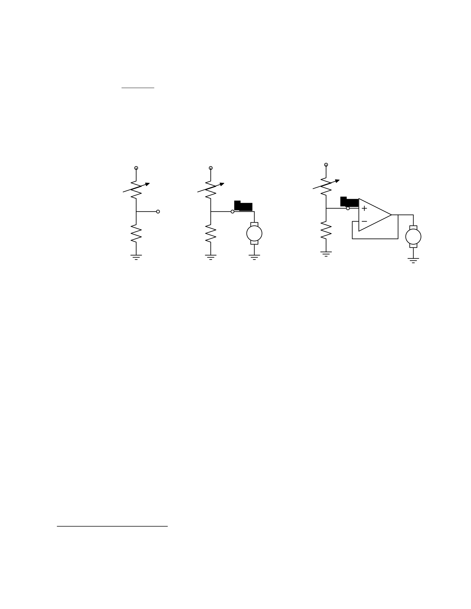
study in detail later in the course, we can determine the following relationship between Vout and
Vin:
RB
Vout = Vin .
RA + RB
So, for example, if RA = RB, then Vout = Vin/2. Or, in our case, if RA actually varies with the amount
of light shining on it, then Vout will also vary with the light.
5
Vin Vin Vin
RARARA
Vout
RBRBmotor RBmotor
Figure 1.3 Voltage dividers: A. Resistor divider. B. Connected to a motor, in a way that breaks
the abstraction from part A. C. Connected to a motor, with a buffer.
That is great. So, now, we might imagine that we could use this voltage difference that we have
created to drive the motor at different speeds, depending on the light hitting the resistor, using
a circuit something like the one shown in figure 1.3B. But, sadly, that will not work. It turns out
that once we connect the motor to the circuit, it actually changes the voltages, and we can no
longer maintain the voltage difference needed to drive the motor.
So, although we have developed an abstract model of the behavior of circuit components, which
lets us analyze the behavior of a particular complete circuit design, it does not give us
modularity. That is, we cannot design two parts of a circuit, understand each of their behaviors,
and then predict the behavior of the composite system based on the behavior of the separate
components. Instead, we would have to re-analyze the joint behavior of the whole composite
system. Lack of modularity makes it very difficult to design large systems, because two different
people, or the same person at two different times, cannot design pieces and put them together
without understanding the whole.
To solve this problem, we can augment our analog-circuit toolbox with some additional
components that allow us to design components with modular behavior; they “buffer” or
“isolate” one part of the circuit from another in ways that allow us to combine the parts more
5
Do not worry if this example does not make much sense to you; we will explore this all in great detail later.

easily. In this class, we will use op-amps to build buffers, which will let us solve our sample
problem using a slightly more complex circuit, as shown in figure 1.3C.
Thus, the key point is that good modules preserve abstraction barriers between the use of a
module and internal details of how they are constructed. We will see this theme recur as we
discuss different PCAP systems.
Digital circuits
In analog circuits, we think about voltages on terminals ranging over real values. This gives us
the freedom to create an enormous variety of circuits, but sometimes that freedom actually
makes the design process more difficult. To design ever more complex circuits, we can move to
a much stronger, digital abstraction, in which the voltages on the terminals are thought of as
only taking on values that are either “low” or “high” (often called 0 and 1). This PCAP system is
made up of a basis set of elements, called gates, that are built out of simpler analog circuit
components, such as transistors and resistors. Adopting the digital abstraction is a huge
limitation on the kinds of circuits that can be built. However, digital circuits can be easy to design
and build and also can be inexpensive because the basic elements (gates) are simple (fewer
transisters are need to construct a gate than to construct an op amp), versatile (only a small
number of different kinds of logic elements are necessary to construct an arbitrary digital
circuit), and combinations are easy to think about (using Boolean logic). These properties allow
designers to build incredibly complex machines by designing small parts and putting them
together into increasingly larger pieces. Digital watches, calculators, and computers are all built
this way.
Digital design is a very important part of EECS, and it is treated in a number of our courses at
basic and advanced levels, but is not one of the topics we will go into in detail in 6.01.
Nevertheless, the same central points that we explore in this course apply to this domain as
well.
Computers
One of the most important developments in the design of digital circuits is that of the
generalpurpose “stored program” computer. Computers are a particular class of digital circuits
that are general purpose: the same actual circuit can perform (almost) any transformation
between its inputs and its outputs. Which particular transformation it performs is governed by
a program, which is some settings of physical switches, or information written on an external
physical memory, such as cards or a tape, or information stored in some sort of internal memory.
The “almost” in the previous section refers to the actual memory capacity of the computer.
Exactly what computations a computer can perform depends on the amount of memory it has;
and also on the time you are willing to wait. So, although a general-purpose computer can do
anything a special-purpose digital circuit can do, in the information-processing sense, the
computer might be slower or use more power. However, using general-purpose computers can
save an enormous amount of engineering time and effort. It is much cheaper and easier to
debug and modify and manufacture software than hardware. The modularities and abstractions
that software PCAP systems give us are even more powerful than those derived from the digital
circuit abstraction.

Again, we can see how abstraction separates use from details; we don’t need to know how the
circuits inside a computer are designed, we just need to know the rules by which we can use
them and the constraints under which they perform.
Python programs
Every general-purpose computer has a different detailed design, which means that the way its
program needs to be specified is different. Furthermore, the “machine languages” for
describing computer programs, at the most primitive level, are awkward for human
programmers. So, we have developed a number of computer programming languages for
specifying a desired computation. These languages are converted into instructions in the
computer’s native machine language by other computer programs, called compilers or
interpreters. One of the coolest and most powerful things about general-purpose computers is
this ability to write computer programs that process or create or modify other computer
programs.
Computer programming languages are PCAP systems. They provide primitive operations, ways
of combining them, ways of abstracting over them, and ways of capturing common abstraction
patterns. We will spend a considerable amount of time in this course studying the particular
primitives, combination mechanisms, and abstraction mechanisms made available in the
Python programming language. But the choice of Python is relatively unimportant. Virtually all
modern programming languages supply a similar set of mechanisms, and the choice of
programming language is primarily a matter of taste and convenience.
In a computer program we have both data primitives and computation primitives. At the most
basic level, computers generally store binary digits (bits) in groups of 32 or 64, called words.
These words are data primitives, and they can be interpreted by our programs as representing
integers, floating-point numbers, strings, or addresses of other data in the computer’s memory.
The computational primitives supported by most computers include numerical operations such
as addition and multiplication, and locating and extracting the contents of a memory at a given
address. In Python, we will work at a level of abstraction that does not require us to think very
much about addresses of data, but it is useful to understand that level of description, as well.
Primitive data and computation elements can be combined and abstracted in a variety of
different ways, depending on choices of programming style. We will explore these in more detail
in section 1.3.2.
1.2.3 Models
So far, we have discussed a number of ways of framing the problem of designing and
constructing mechanisms. Each PCAP system is accompanied by a modeling system that lets us
make mathematical models of the systems we construct.
What is a model? It is a new system that is considerably simpler than the system being modeled,
but which captures the important aspects of the original system. We might make a physical
model of an airplane to test in a wind tunnel. It does not have to have passenger seats or landing
lights; but it has to have surfaces of the correct shape, in order to capture the important
properties for this purpose. Mathematical models can capture properties of systems that are

important to us, and allow us to discover things about the system much more conveniently than
by manipulating the original system itself.
One of the hardest things about building models is deciding which aspects of the original system
to model and which ones to ignore. Many classic, dramatic engineering failures can be ascribed
to failing to model important aspects of the system. One example (which turned out to be an
ethical success story, rather than a failure) is LeMessurier’s Citicorp Building
6
, in which an
engineering design change was made, but tested in a model in which the wind came only from
a limited set of directions.
Another important dimension in modeling is whether the model is deterministic or not. We
might, for example, model the effect of the robot executing a command to set its velocity as
making an instantaneous change to the commanded velocity. But, of course, there is likely to
be some delay and some error. We have to decide whether to ignore that delay and error in our
model and treat it as if it were ideal; or, for example, to make a probabilistic model of the
possible results of that command. Generally speaking, the more different the possible outcomes
of a particular action or command, and the more diffuse the probability distribution over those
outcomes, the more important it is to explicitly include uncertainty in the model.
Once we have a model, we can use it in a variety of different ways, which we explore below.
Analytical models
By far the most prevalent use of models is in analysis: Given a circuit design, what will the
voltage on this terminal be? Given a computer program, will it compute the desired answer?
How long will it take? Given a control system, implemented as a circuit or as a program, will the
system stop at the right distance from the light bulb?
Analytical tools are important. It can be hard to verify the correctness of a system by trying it in
all possible initial conditions with all possible inputs; sometimes it is easier to develop a
mathematical model and then prove a theorem about the model.
For some systems, such as pure software computations, or the addition circuitry in a calculator,
it is possible to analyze correctness or speed with just a model of the system in question. For
other systems, such as fuel injectors, it is impossible to analyze the correctness of the controller
without also modeling the environment (or “plant”) to which it is connected, and then analyzing
the behavior of the coupled system of the controller and environment.
To demonstrate some of these tradeoffs, we can do a very simple analysis of a robot moving
toward a lamp. Imagine that we arrange it so that the robot’s velocity at time t, V[t], is
proportional to the difference between the actual light level, X[t], and a desired light level (that
is, the light level we expect to encounter when the robot is the desired distance from the lamp),
Xdesired ; that is, we can model our control system with the difference equation
6
See “The Fifty-Nine Story Crisis”, The New Yorker, May 29, 1995, pp 45-53.

V[t] = k(Xdesired − X[t]) where k is the constant of
proportionality, or gain, of the controller.
Now, we need to model the world. For simplicity, we equate the light level to the robot’s position
(assuming that the units match); in addition we assume the robot’s position at time t is its
position at time t−1 plus its velocity at time t−1 (actually, this should be the product of the
velocity and the length of time between samples, but we can just assume a unit time step and
thus use velocity). When we couple these models, we get the difference equation
X[t] = X[t − 1] + k(Xdesired − X[t − 1]) .
Now, for a given value of k, we can determine how the system will behave over time, by solving
the difference equation in X.
Later in the course, we will see how easily-determined mathematical properties of a
differenceequation model can tell us whether a control system will have the desired behavior
and whether or not the controller will cause the system to oscillate. These same kinds of
analyses can be applied to robot control systems as well as to the temporal properties of
voltages in a circuit, and even to problems as unrelated as the consequences of a monetary
policy decision in economics. It is important to note that treating the system as moving in
discrete time steps is an approximation to underlying continuous dynamics; it can make models
that are easier to analyze, but it requires sophisticated understanding of sampling to understand
the effects of this approximation on the correctness of the results.
Synthetic models
One goal of many people in a variety of sub-disciplines of computer science and electrical
engineering is automatic synthesis of systems from formal descriptions of their desired
behavior. For example, you might describe some properties you would want the input/output
behavior of a circuit or computer program to have, and then have a computer system discover
a circuit or program with the desired property.
This is a well-specified problem, but generally the search space of possible circuits or programs
is much too large for an automated process; the intuition and previous experience of an expert
human designer cannot yet be matched by computational search methods.
However, humans use informal models of systems for synthesis. The documentation of a
software library, which describes the function of the various procedures, serves as an informal
model that a programmer can use to assemble those components to build new, complex
systems.
Internal models
As we wish to build more and more complex systems with software programs as controllers, we
find that it is often useful to build additional layers of abstraction on top of the one provided by
a generic programming language. This is particularly true when the nature of the exact

computation required depends considerably on information that is only received during the
execution of the system.
Consider, for example, an automated taxi robot (or, more prosaically, the navigation system in
your new car). It takes, as input, a current location in the city and a goal location, and gives, as
output, a path from the current location to the goal. It has a map built into it.
It is theoretically possible to build an enormous digital circuit or computer program that
contains a look-up table, in which we precompute the path for all pairs of locations and store
them away. Then when we want to find a path, we could simply look in the table at the location
corresponding to the start and goal location and retrieve the precomputed path. Unfortunately,
the size of that table is too huge to contemplate. Instead, what we do is construct an abstraction
of the problem as one of finding a path from any start state to any goal state, through a graph
(an abstract mathematical construct of “nodes” with “arcs” connecting them). We can develop
and implement a general-purpose algorithm that will solve any shortest-path problem in a
graph. That algorithm and implementation will be useful for a wide variety of possible problems.
And for the navigation system, all we have to do is represent the map as a graph, specify the
start and goal states, and call the general graph-search algorithm.
We can think of this process as actually putting a model of the system’s interactions with the
world inside the controller; it can consider different courses of action in the world and pick the
one that is the best according to some criterion.
Another example of using internal models is when the system has some significant lack of
information about the state of the environment. In such situations, it may be appropriate to
explicitly model the set of possible states of the external world and their associated
probabilities, and to update this model over time as new evidence is gathered. We will pursue
an example of this approach near the end of the course.
1.3 Programming embedded systems
There are many different ways of thinking about modularity and abstraction for software.
Different models will make some things easier to say and do and others more difficult, making
different models appropriate for different tasks. In the following sections, we explore different
strategies for building software systems that interact with an external environment, and then
different strategies for specifying the purely computational part of a system.
1.3.1 Interacting with the environment
Increasingly, computer systems need to interact with the world around them, receiving
information about the external world, and taking actions to affect the world. Furthermore, the
world is dynamic, so that as the system is computing, the world is changing, requiring future
computation to adapt to the new state of the world.
There are a variety of different ways to organize computations that interact with an external
world. Generally speaking, such a computation needs to:
7. get information from sensors (light sensors, sonars, mouse, keyboard, etc.),
8. perform computation, remembering some of the results, and

9. take actions to change the outside world (move the robot, print, draw, etc.).
These operations can be put together in different styles.
1.3.1.1 Sequential
The most immediately straightforward style for constructing a program that interacts with the
world is the basic imperative style, in which the program gives a sequence of ’commands’ to the
system it is controlling. A library of special procedures is defined, some of which read
information from the sensors and others of which cause actions to be performed. Example
procedures might move a robot forward a fixed distance, or send a file out over the network, or
move video-game characters on the screen.
In this model, we could naturally write a program that moves an idealized robot in a square, if
there is space in front of it.
if noObstacleInFront:
moveDistance(1)
turnAngle(90)
moveDistance(1)
turnAngle(90)
moveDistance(1)
turnAngle(90)
moveDistance(1)
turnAngle(90)
The major problem with this style of programming is that the programmer has to remember to
check the sensors sufficiently frequently. For instance, if the robot checks for free space in front,
and then starts moving, it might turn out that a subsequent sensor reading will show that there
is something in front of the robot, either because someone walked in front of it or because the
previous reading was erroneous. It is hard to have the discipline, as a programmer, to remember
to keep checking the sensor conditions frequently enough, and the resulting programs can be
quite difficult to read and understand.
For the robot moving toward the light, we might write a program like this:
while lightValue <
desiredValue:
moveDistance(0.1)
This would have the robot creep up, step by step, toward the light. We might want to modify it
so that the robot moved a distance that was related to the difference between the current and
desired light values. However, if it takes larger steps, then during the time that it is moving it
will not be sensitive to possible changes in the light value and cannot react immediately to
them.
1.3.1.2 Event-Driven
User-interface programs are often best organized differently, as event-driven (also called
interrupt driven) programs. In this case, the program is specified as a collection of procedures

(called ’handlers’ or ’callbacks’) that are attached to particular events that can take place. So,
for example, there might be procedures that are called when the mouse is clicked on each
button in the interface, when the user types into a text field, or when the temperature of a
reactor gets too high. An “event loop” runs continuously, checking to see whether any of the
triggering events have happened, and, if they have, calling the associated procedure.
In our simple example, we might imagine writing a program that told the robot to drive forward
by default; and then install an event handler that says that if the light level reaches the desired
value, it should stop. This program would be reactive to sudden changes in the environment.
As the number and frequency of the conditions that need responses increases, it can be difficult
to both keep a program like this running well and guarantee a minimum response time to any
event.
1.3.1.3 Transducer
An alternative view is that programming a system that interacts with an external world is like
building a transducer with internal state. Think of a transducer as a processing box that runs
continuously. At regular intervals (perhaps many times per second), the transducer reads all of
the sensors, does a small amount of computation, stores some values it will need for the next
computation, and then generates output values for the actions.
This computation happens over and over and over again. Complex behavior can arise out of the
temporal pattern of inputs and outputs. So, for example, a robot might try to move forward
without hitting something by defining a procedure:
def step(): distToFront = min(frontSonarReadings)
motorOutput(gain * (distToFront - desiredDistance), 0.0)
Executed repeatedly, this program will automatically modulate the robot’s speed to be
proportional to the free space in front of it.
The main problem with the transducer approach is that it can be difficult to do tasks that are
fundamentally sequential (like the example of driving in a square, shown above). We will start
with the transducer model, and then, as described in section 4.3, we will build a new abstraction
layer on top of it that will make it easy to do sequential commands, as well.
1.3.2 Programming models
Just as there are different strategies for organizing entire software systems, there are different
strategies for formally expressing computational processes within those structures.
1.3.2.1 Imperative computation
Most of you have probably been exposed to an imperative model of computer programming, in
which we think of programs as giving a sequential set of instructions to the computer to do
something. And, in fact, that is how the internals of the processors of computers are typically
structured. So, in Java or C or C++, you write typically procedures that consist of lists of
instructions to the computer:

9. Put this value in this variable
10. Square the variable
11. Divide it by pi
12. If the result is greater than 1, return the result
In this model of computation, the primitive computational elements are basic arithmetic
operations and assignment statements. We can combine the elements using sequences of
statements, and control structures such as if, for, and while. We can abstract away from the
details of a computation by defining a procedure that does it. Now, the engineer only needs to
know the specifications of the procedure, but not the implementation details, in order to use
it.
1.3.2.2 Functional computation
Another style of programming is the functional style. In this model, we gain power through
function calls. Rather than telling the computer to do things, we ask it questions: What is 4 + 5?
What is the square root of 6? What is the largest element of the list?
These questions can all be expressed as asking for the value of a function applied to some
arguments. But where do the functions come from? The answer is, from other functions. We
start with some set of basic functions (like “plus”), and use them to construct more complex
functions.
This method would not be powerful without the mechanisms of conditional evaluation and
recursion. Conditional functions ask one question under some conditions and another question
under other conditions. Recursion is a mechanism that lets the definition of a function refer to
the function being defined. Recursion is as powerful as iteration.
In this model of computation, the primitive computational elements are typically basic
arithmetic and list operations. We combine elements using function composition (using the
output of one function as the input to another), if, and recursion. We use function definition as
a method of abstraction, and the idea of higher-order functions (passing functions as arguments
to other functions) as a way of capturing common high-level patterns.
1.3.2.3 Data structures
In either style of asking the computer to do work for us, we have another kind of modularity
and abstraction, which is centered around the organization of data.
At the most primitive level, computers operate on collections of (usually 32 or 64) bits. We can
interpret such a collection of bits as representing different things: a positive integer, a signed
integer, a floating-point number, a Boolean value (true or false), one or more characters, or an
address of some other data in the memory of the computer. Python gives us the ability to work
directly with all of these primitives, except for addresses.
There is only so much you can do with a single number, though. We would like to build computer
programs that operate on representations of documents or maps or circuits or social networks.

To do so, we need to aggregate primitive data elements into more complex data structures.
These can include lists, arrays, dictionaries, and other structures of our own devising.
Here, again, we gain the power of abstraction. We can write programs that do operations on a
data structure representing a social network, for example, without having to worry about the
details of how the social network is represented in terms of bits in the machine.
1.3.2.4 Object-oriented programming: computation + data structures
Object-oriented programming is a style that applies the ideas of modularity and abstraction to
execution and data at the same time.
An object is a data structure, together with a set of procedures that operate on the data. Basic
procedures can be written in an imperative or a functional style, but ultimately there is
imperative assignment to state variables in the object.
One major new type of abstraction in OO programming is “generic” programming. It might be
that all objects have a procedure called print associated with them. So, we can ask any object
to print itself, without having to know how it is implemented. Or, in a graphics system, we might
have a variety of different objects that know their x,y positions on the screen. So each of them
can be asked, in the same way, to say what their position is, even though they might be
represented very differently inside the objects.
In addition, most object-oriented systems support inheritance, which is a way to make new
kinds of objects by saying that they are mostly like another kind of object, but with some
exceptions.
This is another way to take advantage of abstraction.
Programming languages
Python as well as other modern programming languages, such as Java, Ruby and C++, support
all of these programming models. The programmer needs to choose which programming model
best suits the task. This is an issue that we will return to throughout the course.
1.4 Summary
We hope that this course will give you a rich set of conceptual tools and practical techniques,
as well as an appreciation of how math, modeling, and implementation can work together to
enable the design and analysis of complex computational systems that interact with the world.
Acknowledgments
Thanks to Jacob White, Hal Abelson, Tomas Lozano-Perez, Sarah Finney, Sari Canelake, Eric
Grimson, Ike Chuang, and Berthold Horn for useful comments and criticisms, and to Denny
Freeman for significant parts and most of the figures in the linear systems chapter. - LPK
1.1 Goals for 6.01
We have many goals for this course. Our primary goal is for you to learn to appreciate and use the
fundamental design principles of modularity and abstraction in a variety of contexts from electrical

engineering and computer science. To achieve this goal, we will study electrical engineering (EE) and
computer science (CS) largely from the perspective of how to build systems that interact with, and attempt
to control, an external environment. Such systems include everything from low-level controllers like heat
regulators or cardiac pacemakers, to medium-level systems like automated navigation or virtual surgery,
to high-level systems that provide more natural human-computer interfaces.
Our second goal is to show you that making mathematical models of real systems can help in the design
and analysis of those systems; and to give you practice with the difficult step of deciding which aspects of
the real world are important to the problem being solved and how to model them in ways that give insight
into the problem.
We also hope to engage you more actively in the educational process. Most of the work of this course will
not be like typical problems from the end of a chapter. You will work individually and in pairs to solve
problems that are deeper and more open-ended. There will not be a unique right answer. Argument,
explanation, and justification of approach will be more important than the answer. We hope to expose
you to the ubiquity of trade-offs in engineering design: it is rare that an approach will be best in every
dimension; some will excel in one way, others in a different way. Deciding how to make such trade-offs is
a crucial part of engineering.
Another way in which we hope to engage you in the material is by having many of you return to the course
as lab assistants in future semesters. Having a large number of lab assistants in the class means that
students can be given more open-ended problems, and have people around to help them when they are
stuck. Even more importantly, the lab assistants are meant to question the students as they go; to
challenge their understanding and help them see and evaluate a variety of approaches. This process is of
great intellectual value to student and lab assistant alike.
Finally, of course, we have the more typical goals of teaching exciting and important basic material from
electrical engineering and computer science, including modern software engineering, linear systems
analysis, electronic circuits, and decision-making. This material all has an internal elegance and beauty, as
well as crucial role in building modern EE and CS systems.
1.2 Modularity, abstraction, and modeling
Whether proving a theorem by building up from lemmas to basic theorems to more specialized results, or
designing a circuit by building up from components to modules to complex processors, or designing a
software system by building up from generic procedures to classes to class libraries, humans deal with
complexity by exploiting the power of abstraction and modularity. Without such tools, a single person
would be overwhelmed by the complexity of a system, as there is only so much detail that a single person
can consciously manage at a time.
Modularity is the idea of building components that can be re-used; and abstraction is the idea that after
constructing a module (be it software or circuits or gears), most of the details of the module construction
can be ignored and a simpler description used for module interaction (the module computes the square
root, or doubles the voltage, or changes the direction of motion).
Given basic modules, one can move up a level of abstraction and construct a new module by putting
together several previously-built modules, thinking only of their abstract descriptions, and not their
implementations. And, of course, this process can be repeated over many stages. This process gives one

the ability to construct systems with complexity far beyond what would be possible if it were necessary to
understand each component in detail.
Any module can be described in a large number of ways. We might describe the circuitry in a digital watch
in terms of how it behaves as a clock and a stopwatch, or in terms of voltages and currents within the
circuit, or in terms of the heat produced at different parts of the circuitry. Each of these is a different model
of the watch. Different models will be appropriate for different tasks: there is no single correct model.
Rather, each model exposes different dimensions of the system, allowing us to explore many aspects of
the design space of a system, and to trade off different factors in the performance of a system.
The primary theme of this course will be to learn about different methods for building modules out of
primitives, and of building different abstract models of them, so that we can analyze or predict their
behavior, and so we can recombine them into even more complex systems. The same fundamental
principles will apply to software, to control systems, and to circuits.
1.2.1 Example problem
Imagine that you need to make a robot that will roll up close to a light bulb and stop a fixed distance from
it. The first question is, how can we get electrical signals to relate to the physical phenomena of light
readings and robot wheel rotations? There is a large part of electrical engineering related to the design of
physical devices that connect to the physical world in such a way that some electrical property of the
device relates to a physical process in the world. For example, a light-sensitive resistor (photo-resistor) is
a sensor whose resistance changes depending on light intensity impinging on it; a motor is an effector
whose rotor speed is related to the voltage across its two terminals. In this course, we will not examine
the detailed physics of sensors and effectors, but will concentrate on ways of designing systems that use
sensors and effectors to perform both simple and more complicated tasks. To get a robot to stop in front
of a light bulb, the problem will be to find a way to connect the photo-resistor to the motor, so that the
robot will stop at an appropriate distance from the bulb. Thus, we will already use the idea of abstraction
to treat sensors Chapter 1 Course Overview
and effectors as primitive modules whose internal details we can ignore, and whose performance
characteristics we can use as we design systems built on these elements.
1.2.2 An abstraction hierarchy of mechanisms
Given the light-sensitive resistor and the motor, we could find many ways of connecting them, using bits
of metal and ceramic of different kinds, or making some kind of magnetic or mechanical linkages. The
space of possible designs of machines is enormous.
One of the most important things that engineers do, when faced with a set of design problems, is to
standardize on a basis set of components to use to build their systems. There are many reasons for
standardizing on a basis set of components, mostly having to do with efficiency of understanding and of
manufacturing. It is important, as a designer, to develop a repertoire of standard bits and pieces of designs
that you understand well and can put together in various ways to make more complex systems. If you use
the same basis set of components as other designers, you can learn valuable techniques from them, rather
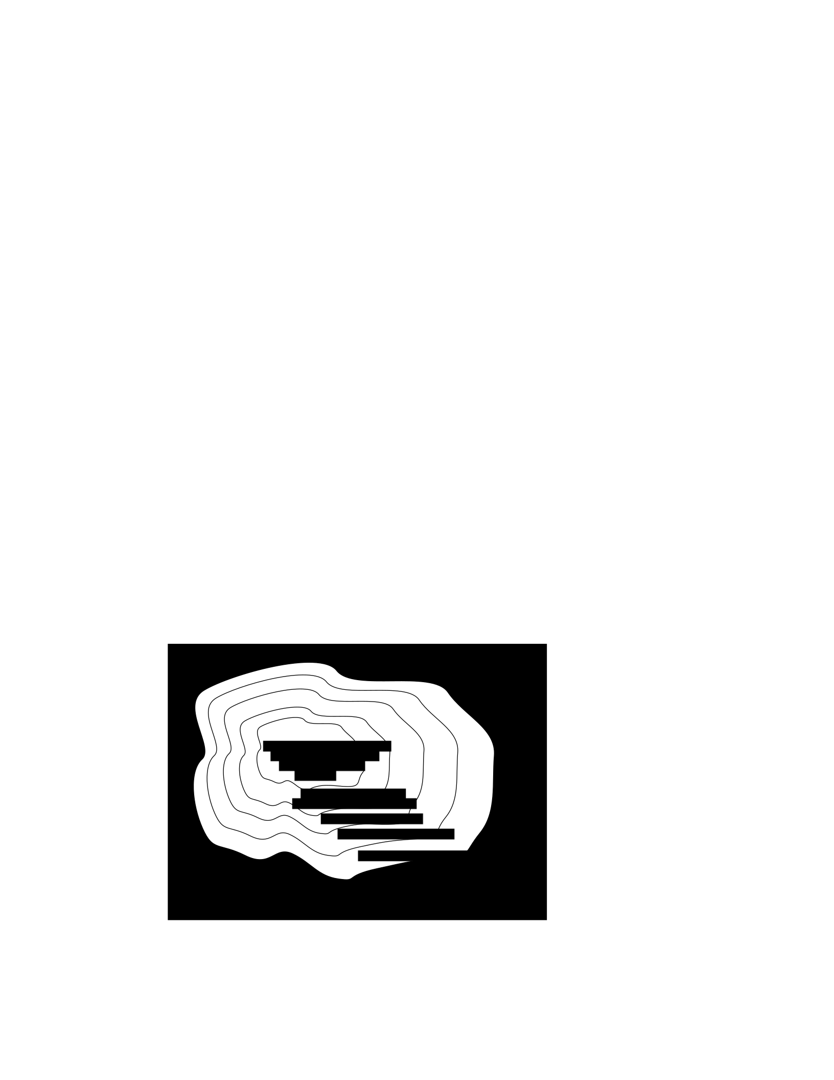
than having to re-invent the techniques yourself. And other people will be able to readily understand and
modify your designs.
We can often make a design job easier by limiting the space of possible designs, and by standardizing on:
• a basis set of primitive components;
• ways of combining the primitive components to make more complex systems;
• ways of “packaging” or abstracting pieces of a design so they can be reused (in essence creating
new “primitives”); and
• ways of capturing common patterns of abstraction (essentially, abstracting our abstractions).
Very complicated design problems can become tractable using such a primitive-combinationabstraction-
pattern (PCAP) approach. In this class, we will examine and learn to use a variety of PCAP strategies
common in EE and CS, and will even design some of our own, for special purposes. In the rest of this
section, we will hint at some of the PCAP systems we will be developing in much greater depth throughout
the class. Figure 1.1 shows one view of this development, as a successive set of restrictions of the design
space of mechanisms.
One very important thing about abstract models is that once we have fixed the abstraction, it will usually
be possible to implement it using a variety of different underlying substrates. So, as shown in figure 1.2,
we can construct general-purpose computers out of a variety of different kinds of systems, including digital
circuits and general-purpose computers. And systems satisfying the digital circuit abstraction can be
constructed from analog circuits, but also from gears or water or light.
Another demonstration of the value of abstracted models is that we can use them, by analogy, to describe
quite different systems. So, for example, the constraint models of circuits that we will study can be applied
to describing transmission of neural signals down the spinal cord, or of heat through a network of
connected bodies.
Let’s explore the abstraction hierarchy figure 1.1 in some more detail, moving up abstraction levels while
observing common patterns.
Figure 1.1 Increasingly constrained systems.
electrical systems
traditional analog circuits
digital electronic circuits
electronic computers
electronic computers
running Python programs
electronic computers with
Python programs that
select outputs by
planning

Figure 1.2 A single abstraction may have a variety of different underlying implementations.
Circuits
Typical electronics circuits are built out of a basis set of primitive components such as voltage sources,
resistors, capacitors, inductors and transistors. This set of component types was chosen to be closely
related to primitive concepts in our physical understanding of electronic systems in terms of voltage,
current, resistance, and the rate of change of those quantities over time. So, when we buy a physical
resistor, we tend to think only of its resistance; and when we buy a capacitor, we think of its ability to store
charge. But, of course, that physical resistor has some capacitance, and the capacitor, some resistance.
Still, it helps us in our designs to have devices that are as close to the ideal models as possible; and it helps
that people have been designing with these components for years, so that we can adopt the strategies
that generations of clever people have developed.
The method of combining circuit elements is to connect their terminals with conductors (wires, crimps,
solder, etc.), a process that is generically referred to as wiring. And our method of abstraction is to describe
the constraints that a circuit element exerts on the currents and voltages of terminals to which the
element is connected.
So, armed with the standard basis set of analog circuit components, we can try to build a circuit to control
our robot. We have a resistance that varies with the light level, but we need a voltage that does so, as well.
We can achieve this by using a voltage divider, which is shown in figure 1.3A. Using an abstract, constraint-
based model of the behavior of circuit components that we will
General-purpose computer
Digital circuits
T
uring
machine
Cellular
automata
Analog
electronics
Gears
Light
W
ater
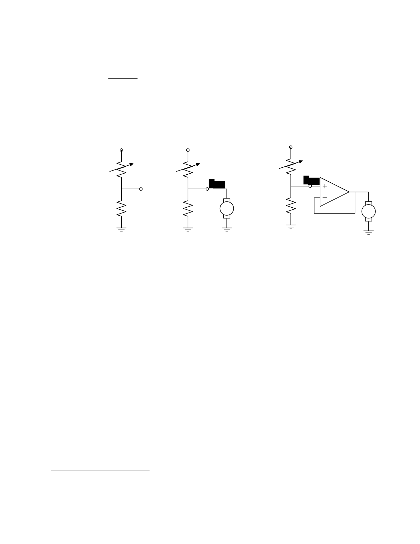
study in detail later in the course, we can determine the following relationship between Vout and
Vin:
RB
Vout = Vin .
RA + RB
So, for example, if RA = RB, then Vout = Vin/2. Or, in our case, if RA actually varies with the amount
of light shining on it, then Vout will also vary with the light.
7
Vin Vin Vin
RARARA
Vout
RBRBmotor RBmotor
Figure 1.3 Voltage dividers: A. Resistor divider. B. Connected to a motor, in a way that breaks
the abstraction from part A. C. Connected to a motor, with a buffer.
That is great. So, now, we might imagine that we could use this voltage difference that we have
created to drive the motor at different speeds, depending on the light hitting the resistor, using
a circuit something like the one shown in figure 1.3B. But, sadly, that will not work. It turns out
that once we connect the motor to the circuit, it actually changes the voltages, and we can no
longer maintain the voltage difference needed to drive the motor.
So, although we have developed an abstract model of the behavior of circuit components, which
lets us analyze the behavior of a particular complete circuit design, it does not give us
modularity. That is, we cannot design two parts of a circuit, understand each of their behaviors,
and then predict the behavior of the composite system based on the behavior of the separate
components. Instead, we would have to re-analyze the joint behavior of the whole composite
system. Lack of modularity makes it very difficult to design large systems, because two different
people, or the same person at two different times, cannot design pieces and put them together
without understanding the whole.
To solve this problem, we can augment our analog-circuit toolbox with some additional
components that allow us to design components with modular behavior; they “buffer” or
“isolate” one part of the circuit from another in ways that allow us to combine the parts more
7
Do not worry if this example does not make much sense to you; we will explore this all in great detail later.

easily. In this class, we will use op-amps to build buffers, which will let us solve our sample
problem using a slightly more complex circuit, as shown in figure 1.3C.
Thus, the key point is that good modules preserve abstraction barriers between the use of a
module and internal details of how they are constructed. We will see this theme recur as we
discuss different PCAP systems.
Digital circuits
In analog circuits, we think about voltages on terminals ranging over real values. This gives us
the freedom to create an enormous variety of circuits, but sometimes that freedom actually
makes the design process more difficult. To design ever more complex circuits, we can move to
a much stronger, digital abstraction, in which the voltages on the terminals are thought of as
only taking on values that are either “low” or “high” (often called 0 and 1). This PCAP system is
made up of a basis set of elements, called gates, that are built out of simpler analog circuit
components, such as transistors and resistors. Adopting the digital abstraction is a huge
limitation on the kinds of circuits that can be built. However, digital circuits can be easy to design
and build and also can be inexpensive because the basic elements (gates) are simple (fewer
transisters are need to construct a gate than to construct an op amp), versatile (only a small
number of different kinds of logic elements are necessary to construct an arbitrary digital
circuit), and combinations are easy to think about (using Boolean logic). These properties allow
designers to build incredibly complex machines by designing small parts and putting them
together into increasingly larger pieces. Digital watches, calculators, and computers are all built
this way.
Digital design is a very important part of EECS, and it is treated in a number of our courses at
basic and advanced levels, but is not one of the topics we will go into in detail in 6.01.
Nevertheless, the same central points that we explore in this course apply to this domain as
well.
Computers
One of the most important developments in the design of digital circuits is that of the
generalpurpose “stored program” computer. Computers are a particular class of digital circuits
that are general purpose: the same actual circuit can perform (almost) any transformation
between its inputs and its outputs. Which particular transformation it performs is governed by
a program, which is some settings of physical switches, or information written on an external
physical memory, such as cards or a tape, or information stored in some sort of internal memory.
The “almost” in the previous section refers to the actual memory capacity of the computer.
Exactly what computations a computer can perform depends on the amount of memory it has;
and also on the time you are willing to wait. So, although a general-purpose computer can do
anything a special-purpose digital circuit can do, in the information-processing sense, the
computer might be slower or use more power. However, using general-purpose computers can
save an enormous amount of engineering time and effort. It is much cheaper and easier to
debug and modify and manufacture software than hardware. The modularities and abstractions
that software PCAP systems give us are even more powerful than those derived from the digital
circuit abstraction.

Again, we can see how abstraction separates use from details; we don’t need to know how the
circuits inside a computer are designed, we just need to know the rules by which we can use
them and the constraints under which they perform.
Python programs
Every general-purpose computer has a different detailed design, which means that the way its
program needs to be specified is different. Furthermore, the “machine languages” for
describing computer programs, at the most primitive level, are awkward for human
programmers. So, we have developed a number of computer programming languages for
specifying a desired computation. These languages are converted into instructions in the
computer’s native machine language by other computer programs, called compilers or
interpreters. One of the coolest and most powerful things about general-purpose computers is
this ability to write computer programs that process or create or modify other computer
programs.
Computer programming languages are PCAP systems. They provide primitive operations, ways
of combining them, ways of abstracting over them, and ways of capturing common abstraction
patterns. We will spend a considerable amount of time in this course studying the particular
primitives, combination mechanisms, and abstraction mechanisms made available in the
Python programming language. But the choice of Python is relatively unimportant. Virtually all
modern programming languages supply a similar set of mechanisms, and the choice of
programming language is primarily a matter of taste and convenience.
In a computer program we have both data primitives and computation primitives. At the most
basic level, computers generally store binary digits (bits) in groups of 32 or 64, called words.
These words are data primitives, and they can be interpreted by our programs as representing
integers, floating-point numbers, strings, or addresses of other data in the computer’s memory.
The computational primitives supported by most computers include numerical operations such
as addition and multiplication, and locating and extracting the contents of a memory at a given
address. In Python, we will work at a level of abstraction that does not require us to think very
much about addresses of data, but it is useful to understand that level of description, as well.
Primitive data and computation elements can be combined and abstracted in a variety of
different ways, depending on choices of programming style. We will explore these in more detail
in section 1.3.2.
1.2.3 Models
So far, we have discussed a number of ways of framing the problem of designing and
constructing mechanisms. Each PCAP system is accompanied by a modeling system that lets us
make mathematical models of the systems we construct.
What is a model? It is a new system that is considerably simpler than the system being modeled,
but which captures the important aspects of the original system. We might make a physical
model of an airplane to test in a wind tunnel. It does not have to have passenger seats or landing
lights; but it has to have surfaces of the correct shape, in order to capture the important
properties for this purpose. Mathematical models can capture properties of systems that are

important to us, and allow us to discover things about the system much more conveniently than
by manipulating the original system itself.
One of the hardest things about building models is deciding which aspects of the original system
to model and which ones to ignore. Many classic, dramatic engineering failures can be ascribed
to failing to model important aspects of the system. One example (which turned out to be an
ethical success story, rather than a failure) is LeMessurier’s Citicorp Building
8
, in which an
engineering design change was made, but tested in a model in which the wind came only from
a limited set of directions.
Another important dimension in modeling is whether the model is deterministic or not. We
might, for example, model the effect of the robot executing a command to set its velocity as
making an instantaneous change to the commanded velocity. But, of course, there is likely to
be some delay and some error. We have to decide whether to ignore that delay and error in our
model and treat it as if it were ideal; or, for example, to make a probabilistic model of the
possible results of that command. Generally speaking, the more different the possible outcomes
of a particular action or command, and the more diffuse the probability distribution over those
outcomes, the more important it is to explicitly include uncertainty in the model.
Once we have a model, we can use it in a variety of different ways, which we explore below.
Analytical models
By far the most prevalent use of models is in analysis: Given a circuit design, what will the
voltage on this terminal be? Given a computer program, will it compute the desired answer?
How long will it take? Given a control system, implemented as a circuit or as a program, will the
system stop at the right distance from the light bulb?
Analytical tools are important. It can be hard to verify the correctness of a system by trying it in
all possible initial conditions with all possible inputs; sometimes it is easier to develop a
mathematical model and then prove a theorem about the model.
For some systems, such as pure software computations, or the addition circuitry in a calculator,
it is possible to analyze correctness or speed with just a model of the system in question. For
other systems, such as fuel injectors, it is impossible to analyze the correctness of the controller
without also modeling the environment (or “plant”) to which it is connected, and then analyzing
the behavior of the coupled system of the controller and environment.
To demonstrate some of these tradeoffs, we can do a very simple analysis of a robot moving
toward a lamp. Imagine that we arrange it so that the robot’s velocity at time t, V[t], is
proportional to the difference between the actual light level, X[t], and a desired light level (that
is, the light level we expect to encounter when the robot is the desired distance from the lamp),
Xdesired ; that is, we can model our control system with the difference equation
8
See “The Fifty-Nine Story Crisis”, The New Yorker, May 29, 1995, pp 45-53.

V[t] = k(Xdesired − X[t]) where k is the constant of
proportionality, or gain, of the controller.
Now, we need to model the world. For simplicity, we equate the light level to the robot’s position
(assuming that the units match); in addition we assume the robot’s position at time t is its
position at time t−1 plus its velocity at time t−1 (actually, this should be the product of the
velocity and the length of time between samples, but we can just assume a unit time step and
thus use velocity). When we couple these models, we get the difference equation
X[t] = X[t − 1] + k(Xdesired − X[t − 1]) .
Now, for a given value of k, we can determine how the system will behave over time, by solving
the difference equation in X.
Later in the course, we will see how easily-determined mathematical properties of a
differenceequation model can tell us whether a control system will have the desired behavior
and whether or not the controller will cause the system to oscillate. These same kinds of
analyses can be applied to robot control systems as well as to the temporal properties of
voltages in a circuit, and even to problems as unrelated as the consequences of a monetary
policy decision in economics. It is important to note that treating the system as moving in
discrete time steps is an approximation to underlying continuous dynamics; it can make models
that are easier to analyze, but it requires sophisticated understanding of sampling to understand
the effects of this approximation on the correctness of the results.
Synthetic models
One goal of many people in a variety of sub-disciplines of computer science and electrical
engineering is automatic synthesis of systems from formal descriptions of their desired
behavior. For example, you might describe some properties you would want the input/output
behavior of a circuit or computer program to have, and then have a computer system discover
a circuit or program with the desired property.
This is a well-specified problem, but generally the search space of possible circuits or programs
is much too large for an automated process; the intuition and previous experience of an expert
human designer cannot yet be matched by computational search methods.
However, humans use informal models of systems for synthesis. The documentation of a
software library, which describes the function of the various procedures, serves as an informal
model that a programmer can use to assemble those components to build new, complex
systems.
Internal models
As we wish to build more and more complex systems with software programs as controllers, we
find that it is often useful to build additional layers of abstraction on top of the one provided by
a generic programming language. This is particularly true when the nature of the exact

computation required depends considerably on information that is only received during the
execution of the system.
Consider, for example, an automated taxi robot (or, more prosaically, the navigation system in
your new car). It takes, as input, a current location in the city and a goal location, and gives, as
output, a path from the current location to the goal. It has a map built into it.
It is theoretically possible to build an enormous digital circuit or computer program that
contains a look-up table, in which we precompute the path for all pairs of locations and store
them away. Then when we want to find a path, we could simply look in the table at the location
corresponding to the start and goal location and retrieve the precomputed path. Unfortunately,
the size of that table is too huge to contemplate. Instead, what we do is construct an abstraction
of the problem as one of finding a path from any start state to any goal state, through a graph
(an abstract mathematical construct of “nodes” with “arcs” connecting them). We can develop
and implement a general-purpose algorithm that will solve any shortest-path problem in a
graph. That algorithm and implementation will be useful for a wide variety of possible problems.
And for the navigation system, all we have to do is represent the map as a graph, specify the
start and goal states, and call the general graph-search algorithm.
We can think of this process as actually putting a model of the system’s interactions with the
world inside the controller; it can consider different courses of action in the world and pick the
one that is the best according to some criterion.
Another example of using internal models is when the system has some significant lack of
information about the state of the environment. In such situations, it may be appropriate to
explicitly model the set of possible states of the external world and their associated
probabilities, and to update this model over time as new evidence is gathered. We will pursue
an example of this approach near the end of the course.
1.3 Programming embedded systems
There are many different ways of thinking about modularity and abstraction for software.
Different models will make some things easier to say and do and others more difficult, making
different models appropriate for different tasks. In the following sections, we explore different
strategies for building software systems that interact with an external environment, and then
different strategies for specifying the purely computational part of a system.
1.3.1 Interacting with the environment
Increasingly, computer systems need to interact with the world around them, receiving
information about the external world, and taking actions to affect the world. Furthermore, the
world is dynamic, so that as the system is computing, the world is changing, requiring future
computation to adapt to the new state of the world.
There are a variety of different ways to organize computations that interact with an external
world. Generally speaking, such a computation needs to:
10. get information from sensors (light sensors, sonars, mouse, keyboard, etc.),
11. perform computation, remembering some of the results, and

12. take actions to change the outside world (move the robot, print, draw, etc.).
These operations can be put together in different styles.
1.3.1.1 Sequential
The most immediately straightforward style for constructing a program that interacts with the
world is the basic imperative style, in which the program gives a sequence of ’commands’ to the
system it is controlling. A library of special procedures is defined, some of which read
information from the sensors and others of which cause actions to be performed. Example
procedures might move a robot forward a fixed distance, or send a file out over the network, or
move video-game characters on the screen.
In this model, we could naturally write a program that moves an idealized robot in a square, if
there is space in front of it.
if noObstacleInFront:
moveDistance(1)
turnAngle(90)
moveDistance(1)
turnAngle(90)
moveDistance(1)
turnAngle(90)
moveDistance(1)
turnAngle(90)
The major problem with this style of programming is that the programmer has to remember to
check the sensors sufficiently frequently. For instance, if the robot checks for free space in front,
and then starts moving, it might turn out that a subsequent sensor reading will show that there
is something in front of the robot, either because someone walked in front of it or because the
previous reading was erroneous. It is hard to have the discipline, as a programmer, to remember
to keep checking the sensor conditions frequently enough, and the resulting programs can be
quite difficult to read and understand.
For the robot moving toward the light, we might write a program like this:
while lightValue <
desiredValue:
moveDistance(0.1)
This would have the robot creep up, step by step, toward the light. We might want to modify it
so that the robot moved a distance that was related to the difference between the current and
desired light values. However, if it takes larger steps, then during the time that it is moving it
will not be sensitive to possible changes in the light value and cannot react immediately to
them.
1.3.1.2 Event-Driven
User-interface programs are often best organized differently, as event-driven (also called
interrupt driven) programs. In this case, the program is specified as a collection of procedures

(called ’handlers’ or ’callbacks’) that are attached to particular events that can take place. So,
for example, there might be procedures that are called when the mouse is clicked on each
button in the interface, when the user types into a text field, or when the temperature of a
reactor gets too high. An “event loop” runs continuously, checking to see whether any of the
triggering events have happened, and, if they have, calling the associated procedure.
In our simple example, we might imagine writing a program that told the robot to drive forward
by default; and then install an event handler that says that if the light level reaches the desired
value, it should stop. This program would be reactive to sudden changes in the environment.
As the number and frequency of the conditions that need responses increases, it can be difficult
to both keep a program like this running well and guarantee a minimum response time to any
event.
1.3.1.3 Transducer
An alternative view is that programming a system that interacts with an external world is like
building a transducer with internal state. Think of a transducer as a processing box that runs
continuously. At regular intervals (perhaps many times per second), the transducer reads all of
the sensors, does a small amount of computation, stores some values it will need for the next
computation, and then generates output values for the actions.
This computation happens over and over and over again. Complex behavior can arise out of the
temporal pattern of inputs and outputs. So, for example, a robot might try to move forward
without hitting something by defining a procedure:
def step(): distToFront = min(frontSonarReadings)
motorOutput(gain * (distToFront - desiredDistance), 0.0)
Executed repeatedly, this program will automatically modulate the robot’s speed to be
proportional to the free space in front of it.
The main problem with the transducer approach is that it can be difficult to do tasks that are
fundamentally sequential (like the example of driving in a square, shown above). We will start
with the transducer model, and then, as described in section 4.3, we will build a new abstraction
layer on top of it that will make it easy to do sequential commands, as well.
1.3.2 Programming models
Just as there are different strategies for organizing entire software systems, there are different
strategies for formally expressing computational processes within those structures.
1.3.2.1 Imperative computation
Most of you have probably been exposed to an imperative model of computer programming, in
which we think of programs as giving a sequential set of instructions to the computer to do
something. And, in fact, that is how the internals of the processors of computers are typically
structured. So, in Java or C or C++, you write typically procedures that consist of lists of
instructions to the computer:

13. Put this value in this variable
14. Square the variable
15. Divide it by pi
16. If the result is greater than 1, return the result
In this model of computation, the primitive computational elements are basic arithmetic
operations and assignment statements. We can combine the elements using sequences of
statements, and control structures such as if, for, and while. We can abstract away from the
details of a computation by defining a procedure that does it. Now, the engineer only needs to
know the specifications of the procedure, but not the implementation details, in order to use
it.
1.3.2.2 Functional computation
Another style of programming is the functional style. In this model, we gain power through
function calls. Rather than telling the computer to do things, we ask it questions: What is 4 + 5?
What is the square root of 6? What is the largest element of the list?
These questions can all be expressed as asking for the value of a function applied to some
arguments. But where do the functions come from? The answer is, from other functions. We
start with some set of basic functions (like “plus”), and use them to construct more complex
functions.
This method would not be powerful without the mechanisms of conditional evaluation and
recursion. Conditional functions ask one question under some conditions and another question
under other conditions. Recursion is a mechanism that lets the definition of a function refer to
the function being defined. Recursion is as powerful as iteration.
In this model of computation, the primitive computational elements are typically basic
arithmetic and list operations. We combine elements using function composition (using the
output of one function as the input to another), if, and recursion. We use function definition as
a method of abstraction, and the idea of higher-order functions (passing functions as arguments
to other functions) as a way of capturing common high-level patterns.
1.3.2.3 Data structures
In either style of asking the computer to do work for us, we have another kind of modularity
and abstraction, which is centered around the organization of data.
At the most primitive level, computers operate on collections of (usually 32 or 64) bits. We can
interpret such a collection of bits as representing different things: a positive integer, a signed
integer, a floating-point number, a Boolean value (true or false), one or more characters, or an
address of some other data in the memory of the computer. Python gives us the ability to work
directly with all of these primitives, except for addresses.
There is only so much you can do with a single number, though. We would like to build computer
programs that operate on representations of documents or maps or circuits or social networks.

To do so, we need to aggregate primitive data elements into more complex data structures.
These can include lists, arrays, dictionaries, and other structures of our own devising.
Here, again, we gain the power of abstraction. We can write programs that do operations on a
data structure representing a social network, for example, without having to worry about the
details of how the social network is represented in terms of bits in the machine.
1.3.2.4 Object-oriented programming: computation + data structures
Object-oriented programming is a style that applies the ideas of modularity and abstraction to
execution and data at the same time.
An object is a data structure, together with a set of procedures that operate on the data. Basic
procedures can be written in an imperative or a functional style, but ultimately there is
imperative assignment to state variables in the object.
One major new type of abstraction in OO programming is “generic” programming. It might be
that all objects have a procedure called print associated with them. So, we can ask any object
to print itself, without having to know how it is implemented. Or, in a graphics system, we might
have a variety of different objects that know their x,y positions on the screen. So each of them
can be asked, in the same way, to say what their position is, even though they might be
represented very differently inside the objects.
In addition, most object-oriented systems support inheritance, which is a way to make new
kinds of objects by saying that they are mostly like another kind of object, but with some
exceptions.
This is another way to take advantage of abstraction.
Programming languages
Python as well as other modern programming languages, such as Java, Ruby and C++, support
all of these programming models. The programmer needs to choose which programming model
best suits the task. This is an issue that we will return to throughout the course.
1.4 Summary
We hope that this course will give you a rich set of conceptual tools and practical techniques,
as well as an appreciation of how math, modeling, and implementation can work together to
enable the design and analysis of complex computational systems that interact with the world.
Acknowledgments
Thanks to Jacob White, Hal Abelson, Tomas Lozano-Perez, Sarah Finney, Sari Canelake, Eric
Grimson, Ike Chuang, and Berthold Horn for useful comments and criticisms, and to Denny
Freeman for significant parts and most of the figures in the linear systems chapter. - LPK
1.1 Goals for 6.01
We have many goals for this course. Our primary goal is for you to learn to appreciate and use the
fundamental design principles of modularity and abstraction in a variety of contexts from electrical

engineering and computer science. To achieve this goal, we will study electrical engineering (EE) and
computer science (CS) largely from the perspective of how to build systems that interact with, and attempt
to control, an external environment. Such systems include everything from low-level controllers like heat
regulators or cardiac pacemakers, to medium-level systems like automated navigation or virtual surgery,
to high-level systems that provide more natural human-computer interfaces.
Our second goal is to show you that making mathematical models of real systems can help in the design
and analysis of those systems; and to give you practice with the difficult step of deciding which aspects of
the real world are important to the problem being solved and how to model them in ways that give insight
into the problem.
We also hope to engage you more actively in the educational process. Most of the work of this course will
not be like typical problems from the end of a chapter. You will work individually and in pairs to solve
problems that are deeper and more open-ended. There will not be a unique right answer. Argument,
explanation, and justification of approach will be more important than the answer. We hope to expose
you to the ubiquity of trade-offs in engineering design: it is rare that an approach will be best in every
dimension; some will excel in one way, others in a different way. Deciding how to make such trade-offs is
a crucial part of engineering.
Another way in which we hope to engage you in the material is by having many of you return to the course
as lab assistants in future semesters. Having a large number of lab assistants in the class means that
students can be given more open-ended problems, and have people around to help them when they are
stuck. Even more importantly, the lab assistants are meant to question the students as they go; to
challenge their understanding and help them see and evaluate a variety of approaches. This process is of
great intellectual value to student and lab assistant alike.
Finally, of course, we have the more typical goals of teaching exciting and important basic material from
electrical engineering and computer science, including modern software engineering, linear systems
analysis, electronic circuits, and decision-making. This material all has an internal elegance and beauty, as
well as crucial role in building modern EE and CS systems.
1.2 Modularity, abstraction, and modeling
Whether proving a theorem by building up from lemmas to basic theorems to more specialized results, or
designing a circuit by building up from components to modules to complex processors, or designing a
software system by building up from generic procedures to classes to class libraries, humans deal with
complexity by exploiting the power of abstraction and modularity. Without such tools, a single person
would be overwhelmed by the complexity of a system, as there is only so much detail that a single person
can consciously manage at a time.
Modularity is the idea of building components that can be re-used; and abstraction is the idea that after
constructing a module (be it software or circuits or gears), most of the details of the module construction
can be ignored and a simpler description used for module interaction (the module computes the square
root, or doubles the voltage, or changes the direction of motion).
Given basic modules, one can move up a level of abstraction and construct a new module by putting
together several previously-built modules, thinking only of their abstract descriptions, and not their
implementations. And, of course, this process can be repeated over many stages. This process gives one

the ability to construct systems with complexity far beyond what would be possible if it were necessary to
understand each component in detail.
Any module can be described in a large number of ways. We might describe the circuitry in a digital watch
in terms of how it behaves as a clock and a stopwatch, or in terms of voltages and currents within the
circuit, or in terms of the heat produced at different parts of the circuitry. Each of these is a different model
of the watch. Different models will be appropriate for different tasks: there is no single correct model.
Rather, each model exposes different dimensions of the system, allowing us to explore many aspects of
the design space of a system, and to trade off different factors in the performance of a system.
The primary theme of this course will be to learn about different methods for building modules out of
primitives, and of building different abstract models of them, so that we can analyze or predict their
behavior, and so we can recombine them into even more complex systems. The same fundamental
principles will apply to software, to control systems, and to circuits.
1.2.1 Example problem
Imagine that you need to make a robot that will roll up close to a light bulb and stop a fixed distance from
it. The first question is, how can we get electrical signals to relate to the physical phenomena of light
readings and robot wheel rotations? There is a large part of electrical engineering related to the design of
physical devices that connect to the physical world in such a way that some electrical property of the
device relates to a physical process in the world. For example, a light-sensitive resistor (photo-resistor) is
a sensor whose resistance changes depending on light intensity impinging on it; a motor is an effector
whose rotor speed is related to the voltage across its two terminals. In this course, we will not examine
the detailed physics of sensors and effectors, but will concentrate on ways of designing systems that use
sensors and effectors to perform both simple and more complicated tasks. To get a robot to stop in front
of a light bulb, the problem will be to find a way to connect the photo-resistor to the motor, so that the
robot will stop at an appropriate distance from the bulb. Thus, we will already use the idea of abstraction
to treat sensors Chapter 1 Course Overview
and effectors as primitive modules whose internal details we can ignore, and whose performance
characteristics we can use as we design systems built on these elements.
1.2.2 An abstraction hierarchy of mechanisms
Given the light-sensitive resistor and the motor, we could find many ways of connecting them, using bits
of metal and ceramic of different kinds, or making some kind of magnetic or mechanical linkages. The
space of possible designs of machines is enormous.
One of the most important things that engineers do, when faced with a set of design problems, is to
standardize on a basis set of components to use to build their systems. There are many reasons for
standardizing on a basis set of components, mostly having to do with efficiency of understanding and of
manufacturing. It is important, as a designer, to develop a repertoire of standard bits and pieces of designs
that you understand well and can put together in various ways to make more complex systems. If you use
the same basis set of components as other designers, you can learn valuable techniques from them, rather
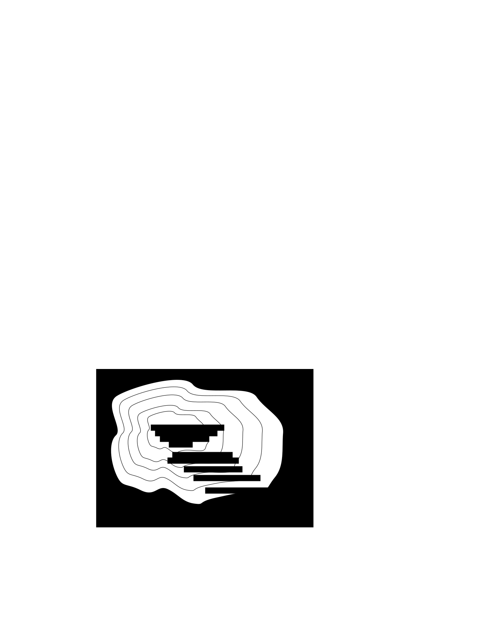
than having to re-invent the techniques yourself. And other people will be able to readily understand and
modify your designs.
We can often make a design job easier by limiting the space of possible designs, and by standardizing on:
• a basis set of primitive components;
• ways of combining the primitive components to make more complex systems;
• ways of “packaging” or abstracting pieces of a design so they can be reused (in essence creating
new “primitives”); and
• ways of capturing common patterns of abstraction (essentially, abstracting our abstractions).
Very complicated design problems can become tractable using such a primitive-combinationabstraction-
pattern (PCAP) approach. In this class, we will examine and learn to use a variety of PCAP strategies
common in EE and CS, and will even design some of our own, for special purposes. In the rest of this
section, we will hint at some of the PCAP systems we will be developing in much greater depth throughout
the class. Figure 1.1 shows one view of this development, as a successive set of restrictions of the design
space of mechanisms.
One very important thing about abstract models is that once we have fixed the abstraction, it will usually
be possible to implement it using a variety of different underlying substrates. So, as shown in figure 1.2,
we can construct general-purpose computers out of a variety of different kinds of systems, including digital
circuits and general-purpose computers. And systems satisfying the digital circuit abstraction can be
constructed from analog circuits, but also from gears or water or light.
Another demonstration of the value of abstracted models is that we can use them, by analogy, to describe
quite different systems. So, for example, the constraint models of circuits that we will study can be applied
to describing transmission of neural signals down the spinal cord, or of heat through a network of
connected bodies.
Let’s explore the abstraction hierarchy figure 1.1 in some more detail, moving up abstraction levels while
observing common patterns.
Figure 1.1 Increasingly constrained systems.
electrical systems
traditional analog circuits
digital electronic circuits
electronic computers
electronic computers
running Python programs
electronic computers with
Python programs that
select outputs by
planning

Figure 1.2 A single abstraction may have a variety of different underlying implementations.
Circuits
Typical electronics circuits are built out of a basis set of primitive components such as voltage sources,
resistors, capacitors, inductors and transistors. This set of component types was chosen to be closely
related to primitive concepts in our physical understanding of electronic systems in terms of voltage,
current, resistance, and the rate of change of those quantities over time. So, when we buy a physical
resistor, we tend to think only of its resistance; and when we buy a capacitor, we think of its ability to store
charge. But, of course, that physical resistor has some capacitance, and the capacitor, some resistance.
Still, it helps us in our designs to have devices that are as close to the ideal models as possible; and it helps
that people have been designing with these components for years, so that we can adopt the strategies
that generations of clever people have developed.
The method of combining circuit elements is to connect their terminals with conductors (wires, crimps,
solder, etc.), a process that is generically referred to as wiring. And our method of abstraction is to describe
the constraints that a circuit element exerts on the currents and voltages of terminals to which the
element is connected.
So, armed with the standard basis set of analog circuit components, we can try to build a circuit to control
our robot. We have a resistance that varies with the light level, but we need a voltage that does so, as well.
We can achieve this by using a voltage divider, which is shown in figure 1.3A. Using an abstract, constraint-
based model of the behavior of circuit components that we will
General-purpose computer
Digital circuits
T
uring
machine
Cellular
automata
Analog
electronics
Gears
Light
W
ater
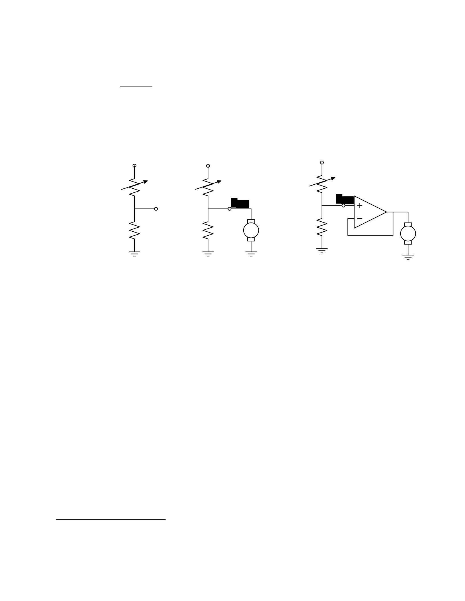
study in detail later in the course, we can determine the following relationship between Vout and
Vin:
RB
Vout = Vin .
RA + RB
So, for example, if RA = RB, then Vout = Vin/2. Or, in our case, if RA actually varies with the amount
of light shining on it, then Vout will also vary with the light.
9
Vin Vin Vin
RARARA
Vout
RBRBmotor RBmotor
Figure 1.3 Voltage dividers: A. Resistor divider. B. Connected to a motor, in a way that breaks
the abstraction from part A. C. Connected to a motor, with a buffer.
That is great. So, now, we might imagine that we could use this voltage difference that we have
created to drive the motor at different speeds, depending on the light hitting the resistor, using
a circuit something like the one shown in figure 1.3B. But, sadly, that will not work. It turns out
that once we connect the motor to the circuit, it actually changes the voltages, and we can no
longer maintain the voltage difference needed to drive the motor.
So, although we have developed an abstract model of the behavior of circuit components, which
lets us analyze the behavior of a particular complete circuit design, it does not give us
modularity. That is, we cannot design two parts of a circuit, understand each of their behaviors,
and then predict the behavior of the composite system based on the behavior of the separate
components. Instead, we would have to re-analyze the joint behavior of the whole composite
system. Lack of modularity makes it very difficult to design large systems, because two different
people, or the same person at two different times, cannot design pieces and put them together
without understanding the whole.
To solve this problem, we can augment our analog-circuit toolbox with some additional
components that allow us to design components with modular behavior; they “buffer” or
“isolate” one part of the circuit from another in ways that allow us to combine the parts more
9
Do not worry if this example does not make much sense to you; we will explore this all in great detail later.

easily. In this class, we will use op-amps to build buffers, which will let us solve our sample
problem using a slightly more complex circuit, as shown in figure 1.3C.
Thus, the key point is that good modules preserve abstraction barriers between the use of a
module and internal details of how they are constructed. We will see this theme recur as we
discuss different PCAP systems.
Digital circuits
In analog circuits, we think about voltages on terminals ranging over real values. This gives us
the freedom to create an enormous variety of circuits, but sometimes that freedom actually
makes the design process more difficult. To design ever more complex circuits, we can move to
a much stronger, digital abstraction, in which the voltages on the terminals are thought of as
only taking on values that are either “low” or “high” (often called 0 and 1). This PCAP system is
made up of a basis set of elements, called gates, that are built out of simpler analog circuit
components, such as transistors and resistors. Adopting the digital abstraction is a huge
limitation on the kinds of circuits that can be built. However, digital circuits can be easy to design
and build and also can be inexpensive because the basic elements (gates) are simple (fewer
transisters are need to construct a gate than to construct an op amp), versatile (only a small
number of different kinds of logic elements are necessary to construct an arbitrary digital
circuit), and combinations are easy to think about (using Boolean logic). These properties allow
designers to build incredibly complex machines by designing small parts and putting them
together into increasingly larger pieces. Digital watches, calculators, and computers are all built
this way.
Digital design is a very important part of EECS, and it is treated in a number of our courses at
basic and advanced levels, but is not one of the topics we will go into in detail in 6.01.
Nevertheless, the same central points that we explore in this course apply to this domain as
well.
Computers
One of the most important developments in the design of digital circuits is that of the
generalpurpose “stored program” computer. Computers are a particular class of digital circuits
that are general purpose: the same actual circuit can perform (almost) any transformation
between its inputs and its outputs. Which particular transformation it performs is governed by
a program, which is some settings of physical switches, or information written on an external
physical memory, such as cards or a tape, or information stored in some sort of internal memory.
The “almost” in the previous section refers to the actual memory capacity of the computer.
Exactly what computations a computer can perform depends on the amount of memory it has;
and also on the time you are willing to wait. So, although a general-purpose computer can do
anything a special-purpose digital circuit can do, in the information-processing sense, the
computer might be slower or use more power. However, using general-purpose computers can
save an enormous amount of engineering time and effort. It is much cheaper and easier to
debug and modify and manufacture software than hardware. The modularities and abstractions
that software PCAP systems give us are even more powerful than those derived from the digital
circuit abstraction.

Again, we can see how abstraction separates use from details; we don’t need to know how the
circuits inside a computer are designed, we just need to know the rules by which we can use
them and the constraints under which they perform.
Python programs
Every general-purpose computer has a different detailed design, which means that the way its
program needs to be specified is different. Furthermore, the “machine languages” for
describing computer programs, at the most primitive level, are awkward for human
programmers. So, we have developed a number of computer programming languages for
specifying a desired computation. These languages are converted into instructions in the
computer’s native machine language by other computer programs, called compilers or
interpreters. One of the coolest and most powerful things about general-purpose computers is
this ability to write computer programs that process or create or modify other computer
programs.
Computer programming languages are PCAP systems. They provide primitive operations, ways
of combining them, ways of abstracting over them, and ways of capturing common abstraction
patterns. We will spend a considerable amount of time in this course studying the particular
primitives, combination mechanisms, and abstraction mechanisms made available in the
Python programming language. But the choice of Python is relatively unimportant. Virtually all
modern programming languages supply a similar set of mechanisms, and the choice of
programming language is primarily a matter of taste and convenience.
In a computer program we have both data primitives and computation primitives. At the most
basic level, computers generally store binary digits (bits) in groups of 32 or 64, called words.
These words are data primitives, and they can be interpreted by our programs as representing
integers, floating-point numbers, strings, or addresses of other data in the computer’s memory.
The computational primitives supported by most computers include numerical operations such
as addition and multiplication, and locating and extracting the contents of a memory at a given
address. In Python, we will work at a level of abstraction that does not require us to think very
much about addresses of data, but it is useful to understand that level of description, as well.
Primitive data and computation elements can be combined and abstracted in a variety of
different ways, depending on choices of programming style. We will explore these in more detail
in section 1.3.2.
1.2.3 Models
So far, we have discussed a number of ways of framing the problem of designing and
constructing mechanisms. Each PCAP system is accompanied by a modeling system that lets us
make mathematical models of the systems we construct.
What is a model? It is a new system that is considerably simpler than the system being modeled,
but which captures the important aspects of the original system. We might make a physical
model of an airplane to test in a wind tunnel. It does not have to have passenger seats or landing
lights; but it has to have surfaces of the correct shape, in order to capture the important
properties for this purpose. Mathematical models can capture properties of systems that are

important to us, and allow us to discover things about the system much more conveniently than
by manipulating the original system itself.
One of the hardest things about building models is deciding which aspects of the original system
to model and which ones to ignore. Many classic, dramatic engineering failures can be ascribed
to failing to model important aspects of the system. One example (which turned out to be an
ethical success story, rather than a failure) is LeMessurier’s Citicorp Building
10
, in which an
engineering design change was made, but tested in a model in which the wind came only from
a limited set of directions.
Another important dimension in modeling is whether the model is deterministic or not. We
might, for example, model the effect of the robot executing a command to set its velocity as
making an instantaneous change to the commanded velocity. But, of course, there is likely to
be some delay and some error. We have to decide whether to ignore that delay and error in our
model and treat it as if it were ideal; or, for example, to make a probabilistic model of the
possible results of that command. Generally speaking, the more different the possible outcomes
of a particular action or command, and the more diffuse the probability distribution over those
outcomes, the more important it is to explicitly include uncertainty in the model.
Once we have a model, we can use it in a variety of different ways, which we explore below.
Analytical models
By far the most prevalent use of models is in analysis: Given a circuit design, what will the
voltage on this terminal be? Given a computer program, will it compute the desired answer?
How long will it take? Given a control system, implemented as a circuit or as a program, will the
system stop at the right distance from the light bulb?
Analytical tools are important. It can be hard to verify the correctness of a system by trying it in
all possible initial conditions with all possible inputs; sometimes it is easier to develop a
mathematical model and then prove a theorem about the model.
For some systems, such as pure software computations, or the addition circuitry in a calculator,
it is possible to analyze correctness or speed with just a model of the system in question. For
other systems, such as fuel injectors, it is impossible to analyze the correctness of the controller
without also modeling the environment (or “plant”) to which it is connected, and then analyzing
the behavior of the coupled system of the controller and environment.
To demonstrate some of these tradeoffs, we can do a very simple analysis of a robot moving
toward a lamp. Imagine that we arrange it so that the robot’s velocity at time t, V[t], is
proportional to the difference between the actual light level, X[t], and a desired light level (that
is, the light level we expect to encounter when the robot is the desired distance from the lamp),
Xdesired ; that is, we can model our control system with the difference equation
10
See “The Fifty-Nine Story Crisis”, The New Yorker, May 29, 1995, pp 45-53.

V[t] = k(Xdesired − X[t]) where k is the constant of
proportionality, or gain, of the controller.
Now, we need to model the world. For simplicity, we equate the light level to the robot’s position
(assuming that the units match); in addition we assume the robot’s position at time t is its
position at time t−1 plus its velocity at time t−1 (actually, this should be the product of the
velocity and the length of time between samples, but we can just assume a unit time step and
thus use velocity). When we couple these models, we get the difference equation
X[t] = X[t − 1] + k(Xdesired − X[t − 1]) .
Now, for a given value of k, we can determine how the system will behave over time, by solving
the difference equation in X.
Later in the course, we will see how easily-determined mathematical properties of a
differenceequation model can tell us whether a control system will have the desired behavior
and whether or not the controller will cause the system to oscillate. These same kinds of
analyses can be applied to robot control systems as well as to the temporal properties of
voltages in a circuit, and even to problems as unrelated as the consequences of a monetary
policy decision in economics. It is important to note that treating the system as moving in
discrete time steps is an approximation to underlying continuous dynamics; it can make models
that are easier to analyze, but it requires sophisticated understanding of sampling to understand
the effects of this approximation on the correctness of the results.
Synthetic models
One goal of many people in a variety of sub-disciplines of computer science and electrical
engineering is automatic synthesis of systems from formal descriptions of their desired
behavior. For example, you might describe some properties you would want the input/output
behavior of a circuit or computer program to have, and then have a computer system discover
a circuit or program with the desired property.
This is a well-specified problem, but generally the search space of possible circuits or programs
is much too large for an automated process; the intuition and previous experience of an expert
human designer cannot yet be matched by computational search methods.
However, humans use informal models of systems for synthesis. The documentation of a
software library, which describes the function of the various procedures, serves as an informal
model that a programmer can use to assemble those components to build new, complex
systems.
Internal models
As we wish to build more and more complex systems with software programs as controllers, we
find that it is often useful to build additional layers of abstraction on top of the one provided by
a generic programming language. This is particularly true when the nature of the exact

computation required depends considerably on information that is only received during the
execution of the system.
Consider, for example, an automated taxi robot (or, more prosaically, the navigation system in
your new car). It takes, as input, a current location in the city and a goal location, and gives, as
output, a path from the current location to the goal. It has a map built into it.
It is theoretically possible to build an enormous digital circuit or computer program that
contains a look-up table, in which we precompute the path for all pairs of locations and store
them away. Then when we want to find a path, we could simply look in the table at the location
corresponding to the start and goal location and retrieve the precomputed path. Unfortunately,
the size of that table is too huge to contemplate. Instead, what we do is construct an abstraction
of the problem as one of finding a path from any start state to any goal state, through a graph
(an abstract mathematical construct of “nodes” with “arcs” connecting them). We can develop
and implement a general-purpose algorithm that will solve any shortest-path problem in a
graph. That algorithm and implementation will be useful for a wide variety of possible problems.
And for the navigation system, all we have to do is represent the map as a graph, specify the
start and goal states, and call the general graph-search algorithm.
We can think of this process as actually putting a model of the system’s interactions with the
world inside the controller; it can consider different courses of action in the world and pick the
one that is the best according to some criterion.
Another example of using internal models is when the system has some significant lack of
information about the state of the environment. In such situations, it may be appropriate to
explicitly model the set of possible states of the external world and their associated
probabilities, and to update this model over time as new evidence is gathered. We will pursue
an example of this approach near the end of the course.
1.3 Programming embedded systems
There are many different ways of thinking about modularity and abstraction for software.
Different models will make some things easier to say and do and others more difficult, making
different models appropriate for different tasks. In the following sections, we explore different
strategies for building software systems that interact with an external environment, and then
different strategies for specifying the purely computational part of a system.
1.3.1 Interacting with the environment
Increasingly, computer systems need to interact with the world around them, receiving
information about the external world, and taking actions to affect the world. Furthermore, the
world is dynamic, so that as the system is computing, the world is changing, requiring future
computation to adapt to the new state of the world.
There are a variety of different ways to organize computations that interact with an external
world. Generally speaking, such a computation needs to:
13. get information from sensors (light sensors, sonars, mouse, keyboard, etc.),
14. perform computation, remembering some of the results, and

15. take actions to change the outside world (move the robot, print, draw, etc.).
These operations can be put together in different styles.
1.3.1.1 Sequential
The most immediately straightforward style for constructing a program that interacts with the
world is the basic imperative style, in which the program gives a sequence of ’commands’ to the
system it is controlling. A library of special procedures is defined, some of which read
information from the sensors and others of which cause actions to be performed. Example
procedures might move a robot forward a fixed distance, or send a file out over the network, or
move video-game characters on the screen.
In this model, we could naturally write a program that moves an idealized robot in a square, if
there is space in front of it.
if noObstacleInFront:
moveDistance(1)
turnAngle(90)
moveDistance(1)
turnAngle(90)
moveDistance(1)
turnAngle(90)
moveDistance(1)
turnAngle(90)
The major problem with this style of programming is that the programmer has to remember to
check the sensors sufficiently frequently. For instance, if the robot checks for free space in front,
and then starts moving, it might turn out that a subsequent sensor reading will show that there
is something in front of the robot, either because someone walked in front of it or because the
previous reading was erroneous. It is hard to have the discipline, as a programmer, to remember
to keep checking the sensor conditions frequently enough, and the resulting programs can be
quite difficult to read and understand.
For the robot moving toward the light, we might write a program like this:
while lightValue <
desiredValue:
moveDistance(0.1)
This would have the robot creep up, step by step, toward the light. We might want to modify it
so that the robot moved a distance that was related to the difference between the current and
desired light values. However, if it takes larger steps, then during the time that it is moving it
will not be sensitive to possible changes in the light value and cannot react immediately to
them.
1.3.1.2 Event-Driven
User-interface programs are often best organized differently, as event-driven (also called
interrupt driven) programs. In this case, the program is specified as a collection of procedures

(called ’handlers’ or ’callbacks’) that are attached to particular events that can take place. So,
for example, there might be procedures that are called when the mouse is clicked on each
button in the interface, when the user types into a text field, or when the temperature of a
reactor gets too high. An “event loop” runs continuously, checking to see whether any of the
triggering events have happened, and, if they have, calling the associated procedure.
In our simple example, we might imagine writing a program that told the robot to drive forward
by default; and then install an event handler that says that if the light level reaches the desired
value, it should stop. This program would be reactive to sudden changes in the environment.
As the number and frequency of the conditions that need responses increases, it can be difficult
to both keep a program like this running well and guarantee a minimum response time to any
event.
1.3.1.3 Transducer
An alternative view is that programming a system that interacts with an external world is like
building a transducer with internal state. Think of a transducer as a processing box that runs
continuously. At regular intervals (perhaps many times per second), the transducer reads all of
the sensors, does a small amount of computation, stores some values it will need for the next
computation, and then generates output values for the actions.
This computation happens over and over and over again. Complex behavior can arise out of the
temporal pattern of inputs and outputs. So, for example, a robot might try to move forward
without hitting something by defining a procedure:
def step(): distToFront = min(frontSonarReadings)
motorOutput(gain * (distToFront - desiredDistance), 0.0)
Executed repeatedly, this program will automatically modulate the robot’s speed to be
proportional to the free space in front of it.
The main problem with the transducer approach is that it can be difficult to do tasks that are
fundamentally sequential (like the example of driving in a square, shown above). We will start
with the transducer model, and then, as described in section 4.3, we will build a new abstraction
layer on top of it that will make it easy to do sequential commands, as well.
1.3.2 Programming models
Just as there are different strategies for organizing entire software systems, there are different
strategies for formally expressing computational processes within those structures.
1.3.2.1 Imperative computation
Most of you have probably been exposed to an imperative model of computer programming, in
which we think of programs as giving a sequential set of instructions to the computer to do
something. And, in fact, that is how the internals of the processors of computers are typically
structured. So, in Java or C or C++, you write typically procedures that consist of lists of
instructions to the computer:

17. Put this value in this variable
18. Square the variable
19. Divide it by pi
20. If the result is greater than 1, return the result
In this model of computation, the primitive computational elements are basic arithmetic
operations and assignment statements. We can combine the elements using sequences of
statements, and control structures such as if, for, and while. We can abstract away from the
details of a computation by defining a procedure that does it. Now, the engineer only needs to
know the specifications of the procedure, but not the implementation details, in order to use
it.
1.3.2.2 Functional computation
Another style of programming is the functional style. In this model, we gain power through
function calls. Rather than telling the computer to do things, we ask it questions: What is 4 + 5?
What is the square root of 6? What is the largest element of the list?
These questions can all be expressed as asking for the value of a function applied to some
arguments. But where do the functions come from? The answer is, from other functions. We
start with some set of basic functions (like “plus”), and use them to construct more complex
functions.
This method would not be powerful without the mechanisms of conditional evaluation and
recursion. Conditional functions ask one question under some conditions and another question
under other conditions. Recursion is a mechanism that lets the definition of a function refer to
the function being defined. Recursion is as powerful as iteration.
In this model of computation, the primitive computational elements are typically basic
arithmetic and list operations. We combine elements using function composition (using the
output of one function as the input to another), if, and recursion. We use function definition as
a method of abstraction, and the idea of higher-order functions (passing functions as arguments
to other functions) as a way of capturing common high-level patterns.
1.3.2.3 Data structures
In either style of asking the computer to do work for us, we have another kind of modularity
and abstraction, which is centered around the organization of data.
At the most primitive level, computers operate on collections of (usually 32 or 64) bits. We can
interpret such a collection of bits as representing different things: a positive integer, a signed
integer, a floating-point number, a Boolean value (true or false), one or more characters, or an
address of some other data in the memory of the computer. Python gives us the ability to work
directly with all of these primitives, except for addresses.
There is only so much you can do with a single number, though. We would like to build computer
programs that operate on representations of documents or maps or circuits or social networks.

To do so, we need to aggregate primitive data elements into more complex data structures.
These can include lists, arrays, dictionaries, and other structures of our own devising.
Here, again, we gain the power of abstraction. We can write programs that do operations on a
data structure representing a social network, for example, without having to worry about the
details of how the social network is represented in terms of bits in the machine.
1.3.2.4 Object-oriented programming: computation + data structures
Object-oriented programming is a style that applies the ideas of modularity and abstraction to
execution and data at the same time.
An object is a data structure, together with a set of procedures that operate on the data. Basic
procedures can be written in an imperative or a functional style, but ultimately there is
imperative assignment to state variables in the object.
One major new type of abstraction in OO programming is “generic” programming. It might be
that all objects have a procedure called print associated with them. So, we can ask any object
to print itself, without having to know how it is implemented. Or, in a graphics system, we might
have a variety of different objects that know their x,y positions on the screen. So each of them
can be asked, in the same way, to say what their position is, even though they might be
represented very differently inside the objects.
In addition, most object-oriented systems support inheritance, which is a way to make new
kinds of objects by saying that they are mostly like another kind of object, but with some
exceptions.
This is another way to take advantage of abstraction.
Programming languages
Python as well as other modern programming languages, such as Java, Ruby and C++, support
all of these programming models. The programmer needs to choose which programming model
best suits the task. This is an issue that we will return to throughout the course.
1.4 Summary
We hope that this course will give you a rich set of conceptual tools and practical techniques,
as well as an appreciation of how math, modeling, and implementation can work together to
enable the design and analysis of complex computational systems that interact with the world.
Acknowledgments
Thanks to Jacob White, Hal Abelson, Tomas Lozano-Perez, Sarah Finney, Sari Canelake, Eric
Grimson, Ike Chuang, and Berthold Horn for useful comments and criticisms, and to Denny
Freeman for significant parts and most of the figures in the linear systems chapter. - LPK
1.1 Goals for 6.01
We have many goals for this course. Our primary goal is for you to learn to appreciate and use the
fundamental design principles of modularity and abstraction in a variety of contexts from electrical

engineering and computer science. To achieve this goal, we will study electrical engineering (EE) and
computer science (CS) largely from the perspective of how to build systems that interact with, and attempt
to control, an external environment. Such systems include everything from low-level controllers like heat
regulators or cardiac pacemakers, to medium-level systems like automated navigation or virtual surgery,
to high-level systems that provide more natural human-computer interfaces.
Our second goal is to show you that making mathematical models of real systems can help in the design
and analysis of those systems; and to give you practice with the difficult step of deciding which aspects of
the real world are important to the problem being solved and how to model them in ways that give insight
into the problem.
We also hope to engage you more actively in the educational process. Most of the work of this course will
not be like typical problems from the end of a chapter. You will work individually and in pairs to solve
problems that are deeper and more open-ended. There will not be a unique right answer. Argument,
explanation, and justification of approach will be more important than the answer. We hope to expose
you to the ubiquity of trade-offs in engineering design: it is rare that an approach will be best in every
dimension; some will excel in one way, others in a different way. Deciding how to make such trade-offs is
a crucial part of engineering.
Another way in which we hope to engage you in the material is by having many of you return to the course
as lab assistants in future semesters. Having a large number of lab assistants in the class means that
students can be given more open-ended problems, and have people around to help them when they are
stuck. Even more importantly, the lab assistants are meant to question the students as they go; to
challenge their understanding and help them see and evaluate a variety of approaches. This process is of
great intellectual value to student and lab assistant alike.
Finally, of course, we have the more typical goals of teaching exciting and important basic material from
electrical engineering and computer science, including modern software engineering, linear systems
analysis, electronic circuits, and decision-making. This material all has an internal elegance and beauty, as
well as crucial role in building modern EE and CS systems.
1.2 Modularity, abstraction, and modeling
Whether proving a theorem by building up from lemmas to basic theorems to more specialized results, or
designing a circuit by building up from components to modules to complex processors, or designing a
software system by building up from generic procedures to classes to class libraries, humans deal with
complexity by exploiting the power of abstraction and modularity. Without such tools, a single person
would be overwhelmed by the complexity of a system, as there is only so much detail that a single person
can consciously manage at a time.
Modularity is the idea of building components that can be re-used; and abstraction is the idea that after
constructing a module (be it software or circuits or gears), most of the details of the module construction
can be ignored and a simpler description used for module interaction (the module computes the square
root, or doubles the voltage, or changes the direction of motion).
Given basic modules, one can move up a level of abstraction and construct a new module by putting
together several previously-built modules, thinking only of their abstract descriptions, and not their
implementations. And, of course, this process can be repeated over many stages. This process gives one

the ability to construct systems with complexity far beyond what would be possible if it were necessary to
understand each component in detail.
Any module can be described in a large number of ways. We might describe the circuitry in a digital watch
in terms of how it behaves as a clock and a stopwatch, or in terms of voltages and currents within the
circuit, or in terms of the heat produced at different parts of the circuitry. Each of these is a different model
of the watch. Different models will be appropriate for different tasks: there is no single correct model.
Rather, each model exposes different dimensions of the system, allowing us to explore many aspects of
the design space of a system, and to trade off different factors in the performance of a system.
The primary theme of this course will be to learn about different methods for building modules out of
primitives, and of building different abstract models of them, so that we can analyze or predict their
behavior, and so we can recombine them into even more complex systems. The same fundamental
principles will apply to software, to control systems, and to circuits.
1.2.1 Example problem
Imagine that you need to make a robot that will roll up close to a light bulb and stop a fixed distance from
it. The first question is, how can we get electrical signals to relate to the physical phenomena of light
readings and robot wheel rotations? There is a large part of electrical engineering related to the design of
physical devices that connect to the physical world in such a way that some electrical property of the
device relates to a physical process in the world. For example, a light-sensitive resistor (photo-resistor) is
a sensor whose resistance changes depending on light intensity impinging on it; a motor is an effector
whose rotor speed is related to the voltage across its two terminals. In this course, we will not examine
the detailed physics of sensors and effectors, but will concentrate on ways of designing systems that use
sensors and effectors to perform both simple and more complicated tasks. To get a robot to stop in front
of a light bulb, the problem will be to find a way to connect the photo-resistor to the motor, so that the
robot will stop at an appropriate distance from the bulb. Thus, we will already use the idea of abstraction
to treat sensors Chapter 1 Course Overview
and effectors as primitive modules whose internal details we can ignore, and whose performance
characteristics we can use as we design systems built on these elements.
1.2.2 An abstraction hierarchy of mechanisms
Given the light-sensitive resistor and the motor, we could find many ways of connecting them, using bits
of metal and ceramic of different kinds, or making some kind of magnetic or mechanical linkages. The
space of possible designs of machines is enormous.
One of the most important things that engineers do, when faced with a set of design problems, is to
standardize on a basis set of components to use to build their systems. There are many reasons for
standardizing on a basis set of components, mostly having to do with efficiency of understanding and of
manufacturing. It is important, as a designer, to develop a repertoire of standard bits and pieces of designs
that you understand well and can put together in various ways to make more complex systems. If you use
the same basis set of components as other designers, you can learn valuable techniques from them, rather
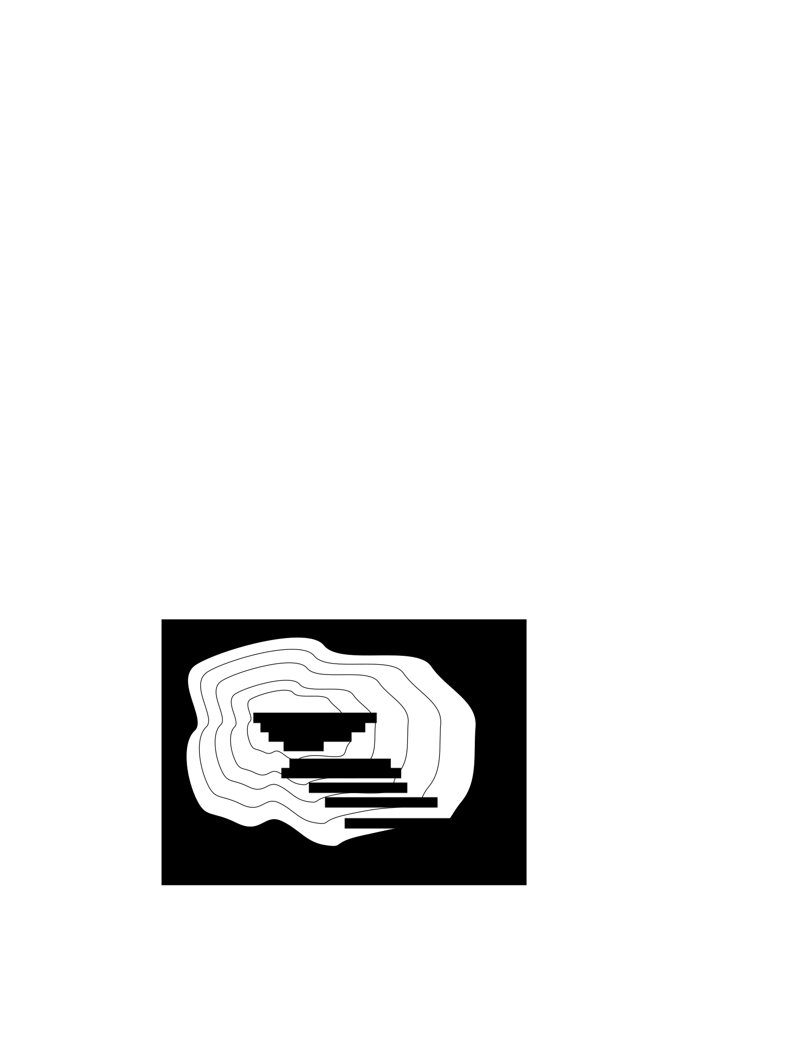
than having to re-invent the techniques yourself. And other people will be able to readily understand and
modify your designs.
We can often make a design job easier by limiting the space of possible designs, and by standardizing on:
• a basis set of primitive components;
• ways of combining the primitive components to make more complex systems;
• ways of “packaging” or abstracting pieces of a design so they can be reused (in essence creating
new “primitives”); and
• ways of capturing common patterns of abstraction (essentially, abstracting our abstractions).
Very complicated design problems can become tractable using such a primitive-combinationabstraction-
pattern (PCAP) approach. In this class, we will examine and learn to use a variety of PCAP strategies
common in EE and CS, and will even design some of our own, for special purposes. In the rest of this
section, we will hint at some of the PCAP systems we will be developing in much greater depth throughout
the class. Figure 1.1 shows one view of this development, as a successive set of restrictions of the design
space of mechanisms.
One very important thing about abstract models is that once we have fixed the abstraction, it will usually
be possible to implement it using a variety of different underlying substrates. So, as shown in figure 1.2,
we can construct general-purpose computers out of a variety of different kinds of systems, including digital
circuits and general-purpose computers. And systems satisfying the digital circuit abstraction can be
constructed from analog circuits, but also from gears or water or light.
Another demonstration of the value of abstracted models is that we can use them, by analogy, to describe
quite different systems. So, for example, the constraint models of circuits that we will study can be applied
to describing transmission of neural signals down the spinal cord, or of heat through a network of
connected bodies.
Let’s explore the abstraction hierarchy figure 1.1 in some more detail, moving up abstraction levels while
observing common patterns.
Figure 1.1 Increasingly constrained systems.
electrical systems
traditional analog circuits
digital electronic circuits
electronic computers
electronic computers
running Python programs
electronic computers with
Python programs that
select outputs by
planning

Figure 1.2 A single abstraction may have a variety of different underlying implementations.
Circuits
Typical electronics circuits are built out of a basis set of primitive components such as voltage sources,
resistors, capacitors, inductors and transistors. This set of component types was chosen to be closely
related to primitive concepts in our physical understanding of electronic systems in terms of voltage,
current, resistance, and the rate of change of those quantities over time. So, when we buy a physical
resistor, we tend to think only of its resistance; and when we buy a capacitor, we think of its ability to store
charge. But, of course, that physical resistor has some capacitance, and the capacitor, some resistance.
Still, it helps us in our designs to have devices that are as close to the ideal models as possible; and it helps
that people have been designing with these components for years, so that we can adopt the strategies
that generations of clever people have developed.
The method of combining circuit elements is to connect their terminals with conductors (wires, crimps,
solder, etc.), a process that is generically referred to as wiring. And our method of abstraction is to describe
the constraints that a circuit element exerts on the currents and voltages of terminals to which the
element is connected.
So, armed with the standard basis set of analog circuit components, we can try to build a circuit to control
our robot. We have a resistance that varies with the light level, but we need a voltage that does so, as well.
We can achieve this by using a voltage divider, which is shown in figure 1.3A. Using an abstract, constraint-
based model of the behavior of circuit components that we will
General-purpose computer
Digital circuits
T
uring
machine
Cellular
automata
Analog
electronics
Gears
Light
W
ater
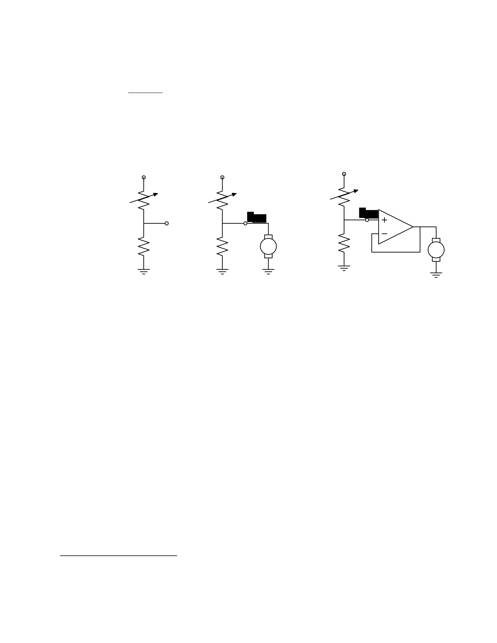
study in detail later in the course, we can determine the following relationship between Vout and
Vin:
RB
Vout = Vin .
RA + RB
So, for example, if RA = RB, then Vout = Vin/2. Or, in our case, if RA actually varies with the amount
of light shining on it, then Vout will also vary with the light.
11
Vin Vin Vin
RARARA
Vout
RBRBmotor RBmotor
Figure 1.3 Voltage dividers: A. Resistor divider. B. Connected to a motor, in a way that breaks
the abstraction from part A. C. Connected to a motor, with a buffer.
That is great. So, now, we might imagine that we could use this voltage difference that we have
created to drive the motor at different speeds, depending on the light hitting the resistor, using
a circuit something like the one shown in figure 1.3B. But, sadly, that will not work. It turns out
that once we connect the motor to the circuit, it actually changes the voltages, and we can no
longer maintain the voltage difference needed to drive the motor.
So, although we have developed an abstract model of the behavior of circuit components, which
lets us analyze the behavior of a particular complete circuit design, it does not give us
modularity. That is, we cannot design two parts of a circuit, understand each of their behaviors,
and then predict the behavior of the composite system based on the behavior of the separate
components. Instead, we would have to re-analyze the joint behavior of the whole composite
system. Lack of modularity makes it very difficult to design large systems, because two different
people, or the same person at two different times, cannot design pieces and put them together
without understanding the whole.
To solve this problem, we can augment our analog-circuit toolbox with some additional
components that allow us to design components with modular behavior; they “buffer” or
“isolate” one part of the circuit from another in ways that allow us to combine the parts more
11
Do not worry if this example does not make much sense to you; we will explore this all in great detail later.

easily. In this class, we will use op-amps to build buffers, which will let us solve our sample
problem using a slightly more complex circuit, as shown in figure 1.3C.
Thus, the key point is that good modules preserve abstraction barriers between the use of a
module and internal details of how they are constructed. We will see this theme recur as we
discuss different PCAP systems.
Digital circuits
In analog circuits, we think about voltages on terminals ranging over real values. This gives us
the freedom to create an enormous variety of circuits, but sometimes that freedom actually
makes the design process more difficult. To design ever more complex circuits, we can move to
a much stronger, digital abstraction, in which the voltages on the terminals are thought of as
only taking on values that are either “low” or “high” (often called 0 and 1). This PCAP system is
made up of a basis set of elements, called gates, that are built out of simpler analog circuit
components, such as transistors and resistors. Adopting the digital abstraction is a huge
limitation on the kinds of circuits that can be built. However, digital circuits can be easy to design
and build and also can be inexpensive because the basic elements (gates) are simple (fewer
transisters are need to construct a gate than to construct an op amp), versatile (only a small
number of different kinds of logic elements are necessary to construct an arbitrary digital
circuit), and combinations are easy to think about (using Boolean logic). These properties allow
designers to build incredibly complex machines by designing small parts and putting them
together into increasingly larger pieces. Digital watches, calculators, and computers are all built
this way.
Digital design is a very important part of EECS, and it is treated in a number of our courses at
basic and advanced levels, but is not one of the topics we will go into in detail in 6.01.
Nevertheless, the same central points that we explore in this course apply to this domain as
well.
Computers
One of the most important developments in the design of digital circuits is that of the
generalpurpose “stored program” computer. Computers are a particular class of digital circuits
that are general purpose: the same actual circuit can perform (almost) any transformation
between its inputs and its outputs. Which particular transformation it performs is governed by
a program, which is some settings of physical switches, or information written on an external
physical memory, such as cards or a tape, or information stored in some sort of internal memory.
The “almost” in the previous section refers to the actual memory capacity of the computer.
Exactly what computations a computer can perform depends on the amount of memory it has;
and also on the time you are willing to wait. So, although a general-purpose computer can do
anything a special-purpose digital circuit can do, in the information-processing sense, the
computer might be slower or use more power. However, using general-purpose computers can
save an enormous amount of engineering time and effort. It is much cheaper and easier to
debug and modify and manufacture software than hardware. The modularities and abstractions
that software PCAP systems give us are even more powerful than those derived from the digital
circuit abstraction.

Again, we can see how abstraction separates use from details; we don’t need to know how the
circuits inside a computer are designed, we just need to know the rules by which we can use
them and the constraints under which they perform.
Python programs
Every general-purpose computer has a different detailed design, which means that the way its
program needs to be specified is different. Furthermore, the “machine languages” for
describing computer programs, at the most primitive level, are awkward for human
programmers. So, we have developed a number of computer programming languages for
specifying a desired computation. These languages are converted into instructions in the
computer’s native machine language by other computer programs, called compilers or
interpreters. One of the coolest and most powerful things about general-purpose computers is
this ability to write computer programs that process or create or modify other computer
programs.
Computer programming languages are PCAP systems. They provide primitive operations, ways
of combining them, ways of abstracting over them, and ways of capturing common abstraction
patterns. We will spend a considerable amount of time in this course studying the particular
primitives, combination mechanisms, and abstraction mechanisms made available in the
Python programming language. But the choice of Python is relatively unimportant. Virtually all
modern programming languages supply a similar set of mechanisms, and the choice of
programming language is primarily a matter of taste and convenience.
In a computer program we have both data primitives and computation primitives. At the most
basic level, computers generally store binary digits (bits) in groups of 32 or 64, called words.
These words are data primitives, and they can be interpreted by our programs as representing
integers, floating-point numbers, strings, or addresses of other data in the computer’s memory.
The computational primitives supported by most computers include numerical operations such
as addition and multiplication, and locating and extracting the contents of a memory at a given
address. In Python, we will work at a level of abstraction that does not require us to think very
much about addresses of data, but it is useful to understand that level of description, as well.
Primitive data and computation elements can be combined and abstracted in a variety of
different ways, depending on choices of programming style. We will explore these in more detail
in section 1.3.2.
1.2.3 Models
So far, we have discussed a number of ways of framing the problem of designing and
constructing mechanisms. Each PCAP system is accompanied by a modeling system that lets us
make mathematical models of the systems we construct.
What is a model? It is a new system that is considerably simpler than the system being modeled,
but which captures the important aspects of the original system. We might make a physical
model of an airplane to test in a wind tunnel. It does not have to have passenger seats or landing
lights; but it has to have surfaces of the correct shape, in order to capture the important
properties for this purpose. Mathematical models can capture properties of systems that are

important to us, and allow us to discover things about the system much more conveniently than
by manipulating the original system itself.
One of the hardest things about building models is deciding which aspects of the original system
to model and which ones to ignore. Many classic, dramatic engineering failures can be ascribed
to failing to model important aspects of the system. One example (which turned out to be an
ethical success story, rather than a failure) is LeMessurier’s Citicorp Building
12
, in which an
engineering design change was made, but tested in a model in which the wind came only from
a limited set of directions.
Another important dimension in modeling is whether the model is deterministic or not. We
might, for example, model the effect of the robot executing a command to set its velocity as
making an instantaneous change to the commanded velocity. But, of course, there is likely to
be some delay and some error. We have to decide whether to ignore that delay and error in our
model and treat it as if it were ideal; or, for example, to make a probabilistic model of the
possible results of that command. Generally speaking, the more different the possible outcomes
of a particular action or command, and the more diffuse the probability distribution over those
outcomes, the more important it is to explicitly include uncertainty in the model.
Once we have a model, we can use it in a variety of different ways, which we explore below.
Analytical models
By far the most prevalent use of models is in analysis: Given a circuit design, what will the
voltage on this terminal be? Given a computer program, will it compute the desired answer?
How long will it take? Given a control system, implemented as a circuit or as a program, will the
system stop at the right distance from the light bulb?
Analytical tools are important. It can be hard to verify the correctness of a system by trying it in
all possible initial conditions with all possible inputs; sometimes it is easier to develop a
mathematical model and then prove a theorem about the model.
For some systems, such as pure software computations, or the addition circuitry in a calculator,
it is possible to analyze correctness or speed with just a model of the system in question. For
other systems, such as fuel injectors, it is impossible to analyze the correctness of the controller
without also modeling the environment (or “plant”) to which it is connected, and then analyzing
the behavior of the coupled system of the controller and environment.
To demonstrate some of these tradeoffs, we can do a very simple analysis of a robot moving
toward a lamp. Imagine that we arrange it so that the robot’s velocity at time t, V[t], is
proportional to the difference between the actual light level, X[t], and a desired light level (that
is, the light level we expect to encounter when the robot is the desired distance from the lamp),
Xdesired ; that is, we can model our control system with the difference equation
12
See “The Fifty-Nine Story Crisis”, The New Yorker, May 29, 1995, pp 45-53.

V[t] = k(Xdesired − X[t]) where k is the constant of
proportionality, or gain, of the controller.
Now, we need to model the world. For simplicity, we equate the light level to the robot’s position
(assuming that the units match); in addition we assume the robot’s position at time t is its
position at time t−1 plus its velocity at time t−1 (actually, this should be the product of the
velocity and the length of time between samples, but we can just assume a unit time step and
thus use velocity). When we couple these models, we get the difference equation
X[t] = X[t − 1] + k(Xdesired − X[t − 1]) .
Now, for a given value of k, we can determine how the system will behave over time, by solving
the difference equation in X.
Later in the course, we will see how easily-determined mathematical properties of a
differenceequation model can tell us whether a control system will have the desired behavior
and whether or not the controller will cause the system to oscillate. These same kinds of
analyses can be applied to robot control systems as well as to the temporal properties of
voltages in a circuit, and even to problems as unrelated as the consequences of a monetary
policy decision in economics. It is important to note that treating the system as moving in
discrete time steps is an approximation to underlying continuous dynamics; it can make models
that are easier to analyze, but it requires sophisticated understanding of sampling to understand
the effects of this approximation on the correctness of the results.
Synthetic models
One goal of many people in a variety of sub-disciplines of computer science and electrical
engineering is automatic synthesis of systems from formal descriptions of their desired
behavior. For example, you might describe some properties you would want the input/output
behavior of a circuit or computer program to have, and then have a computer system discover
a circuit or program with the desired property.
This is a well-specified problem, but generally the search space of possible circuits or programs
is much too large for an automated process; the intuition and previous experience of an expert
human designer cannot yet be matched by computational search methods.
However, humans use informal models of systems for synthesis. The documentation of a
software library, which describes the function of the various procedures, serves as an informal
model that a programmer can use to assemble those components to build new, complex
systems.
Internal models
As we wish to build more and more complex systems with software programs as controllers, we
find that it is often useful to build additional layers of abstraction on top of the one provided by
a generic programming language. This is particularly true when the nature of the exact

computation required depends considerably on information that is only received during the
execution of the system.
Consider, for example, an automated taxi robot (or, more prosaically, the navigation system in
your new car). It takes, as input, a current location in the city and a goal location, and gives, as
output, a path from the current location to the goal. It has a map built into it.
It is theoretically possible to build an enormous digital circuit or computer program that
contains a look-up table, in which we precompute the path for all pairs of locations and store
them away. Then when we want to find a path, we could simply look in the table at the location
corresponding to the start and goal location and retrieve the precomputed path. Unfortunately,
the size of that table is too huge to contemplate. Instead, what we do is construct an abstraction
of the problem as one of finding a path from any start state to any goal state, through a graph
(an abstract mathematical construct of “nodes” with “arcs” connecting them). We can develop
and implement a general-purpose algorithm that will solve any shortest-path problem in a
graph. That algorithm and implementation will be useful for a wide variety of possible problems.
And for the navigation system, all we have to do is represent the map as a graph, specify the
start and goal states, and call the general graph-search algorithm.
We can think of this process as actually putting a model of the system’s interactions with the
world inside the controller; it can consider different courses of action in the world and pick the
one that is the best according to some criterion.
Another example of using internal models is when the system has some significant lack of
information about the state of the environment. In such situations, it may be appropriate to
explicitly model the set of possible states of the external world and their associated
probabilities, and to update this model over time as new evidence is gathered. We will pursue
an example of this approach near the end of the course.
1.3 Programming embedded systems
There are many different ways of thinking about modularity and abstraction for software.
Different models will make some things easier to say and do and others more difficult, making
different models appropriate for different tasks. In the following sections, we explore different
strategies for building software systems that interact with an external environment, and then
different strategies for specifying the purely computational part of a system.
1.3.1 Interacting with the environment
Increasingly, computer systems need to interact with the world around them, receiving
information about the external world, and taking actions to affect the world. Furthermore, the
world is dynamic, so that as the system is computing, the world is changing, requiring future
computation to adapt to the new state of the world.
There are a variety of different ways to organize computations that interact with an external
world. Generally speaking, such a computation needs to:
16. get information from sensors (light sensors, sonars, mouse, keyboard, etc.),
17. perform computation, remembering some of the results, and

18. take actions to change the outside world (move the robot, print, draw, etc.).
These operations can be put together in different styles.
1.3.1.1 Sequential
The most immediately straightforward style for constructing a program that interacts with the
world is the basic imperative style, in which the program gives a sequence of ’commands’ to the
system it is controlling. A library of special procedures is defined, some of which read
information from the sensors and others of which cause actions to be performed. Example
procedures might move a robot forward a fixed distance, or send a file out over the network, or
move video-game characters on the screen.
In this model, we could naturally write a program that moves an idealized robot in a square, if
there is space in front of it.
if noObstacleInFront:
moveDistance(1)
turnAngle(90)
moveDistance(1)
turnAngle(90)
moveDistance(1)
turnAngle(90)
moveDistance(1)
turnAngle(90)
The major problem with this style of programming is that the programmer has to remember to
check the sensors sufficiently frequently. For instance, if the robot checks for free space in front,
and then starts moving, it might turn out that a subsequent sensor reading will show that there
is something in front of the robot, either because someone walked in front of it or because the
previous reading was erroneous. It is hard to have the discipline, as a programmer, to remember
to keep checking the sensor conditions frequently enough, and the resulting programs can be
quite difficult to read and understand.
For the robot moving toward the light, we might write a program like this:
while lightValue <
desiredValue:
moveDistance(0.1)
This would have the robot creep up, step by step, toward the light. We might want to modify it
so that the robot moved a distance that was related to the difference between the current and
desired light values. However, if it takes larger steps, then during the time that it is moving it
will not be sensitive to possible changes in the light value and cannot react immediately to
them.
1.3.1.2 Event-Driven
User-interface programs are often best organized differently, as event-driven (also called
interrupt driven) programs. In this case, the program is specified as a collection of procedures

(called ’handlers’ or ’callbacks’) that are attached to particular events that can take place. So,
for example, there might be procedures that are called when the mouse is clicked on each
button in the interface, when the user types into a text field, or when the temperature of a
reactor gets too high. An “event loop” runs continuously, checking to see whether any of the
triggering events have happened, and, if they have, calling the associated procedure.
In our simple example, we might imagine writing a program that told the robot to drive forward
by default; and then install an event handler that says that if the light level reaches the desired
value, it should stop. This program would be reactive to sudden changes in the environment.
As the number and frequency of the conditions that need responses increases, it can be difficult
to both keep a program like this running well and guarantee a minimum response time to any
event.
1.3.1.3 Transducer
An alternative view is that programming a system that interacts with an external world is like
building a transducer with internal state. Think of a transducer as a processing box that runs
continuously. At regular intervals (perhaps many times per second), the transducer reads all of
the sensors, does a small amount of computation, stores some values it will need for the next
computation, and then generates output values for the actions.
This computation happens over and over and over again. Complex behavior can arise out of the
temporal pattern of inputs and outputs. So, for example, a robot might try to move forward
without hitting something by defining a procedure:
def step(): distToFront = min(frontSonarReadings)
motorOutput(gain * (distToFront - desiredDistance), 0.0)
Executed repeatedly, this program will automatically modulate the robot’s speed to be
proportional to the free space in front of it.
The main problem with the transducer approach is that it can be difficult to do tasks that are
fundamentally sequential (like the example of driving in a square, shown above). We will start
with the transducer model, and then, as described in section 4.3, we will build a new abstraction
layer on top of it that will make it easy to do sequential commands, as well.
1.3.2 Programming models
Just as there are different strategies for organizing entire software systems, there are different
strategies for formally expressing computational processes within those structures.
1.3.2.1 Imperative computation
Most of you have probably been exposed to an imperative model of computer programming, in
which we think of programs as giving a sequential set of instructions to the computer to do
something. And, in fact, that is how the internals of the processors of computers are typically
structured. So, in Java or C or C++, you write typically procedures that consist of lists of
instructions to the computer:

21. Put this value in this variable
22. Square the variable
23. Divide it by pi
24. If the result is greater than 1, return the result
In this model of computation, the primitive computational elements are basic arithmetic
operations and assignment statements. We can combine the elements using sequences of
statements, and control structures such as if, for, and while. We can abstract away from the
details of a computation by defining a procedure that does it. Now, the engineer only needs to
know the specifications of the procedure, but not the implementation details, in order to use
it.
1.3.2.2 Functional computation
Another style of programming is the functional style. In this model, we gain power through
function calls. Rather than telling the computer to do things, we ask it questions: What is 4 + 5?
What is the square root of 6? What is the largest element of the list?
These questions can all be expressed as asking for the value of a function applied to some
arguments. But where do the functions come from? The answer is, from other functions. We
start with some set of basic functions (like “plus”), and use them to construct more complex
functions.
This method would not be powerful without the mechanisms of conditional evaluation and
recursion. Conditional functions ask one question under some conditions and another question
under other conditions. Recursion is a mechanism that lets the definition of a function refer to
the function being defined. Recursion is as powerful as iteration.
In this model of computation, the primitive computational elements are typically basic
arithmetic and list operations. We combine elements using function composition (using the
output of one function as the input to another), if, and recursion. We use function definition as
a method of abstraction, and the idea of higher-order functions (passing functions as arguments
to other functions) as a way of capturing common high-level patterns.
1.3.2.3 Data structures
In either style of asking the computer to do work for us, we have another kind of modularity
and abstraction, which is centered around the organization of data.
At the most primitive level, computers operate on collections of (usually 32 or 64) bits. We can
interpret such a collection of bits as representing different things: a positive integer, a signed
integer, a floating-point number, a Boolean value (true or false), one or more characters, or an
address of some other data in the memory of the computer. Python gives us the ability to work
directly with all of these primitives, except for addresses.
There is only so much you can do with a single number, though. We would like to build computer
programs that operate on representations of documents or maps or circuits or social networks.

To do so, we need to aggregate primitive data elements into more complex data structures.
These can include lists, arrays, dictionaries, and other structures of our own devising.
Here, again, we gain the power of abstraction. We can write programs that do operations on a
data structure representing a social network, for example, without having to worry about the
details of how the social network is represented in terms of bits in the machine.
1.3.2.4 Object-oriented programming: computation + data structures
Object-oriented programming is a style that applies the ideas of modularity and abstraction to
execution and data at the same time.
An object is a data structure, together with a set of procedures that operate on the data. Basic
procedures can be written in an imperative or a functional style, but ultimately there is
imperative assignment to state variables in the object.
One major new type of abstraction in OO programming is “generic” programming. It might be
that all objects have a procedure called print associated with them. So, we can ask any object
to print itself, without having to know how it is implemented. Or, in a graphics system, we might
have a variety of different objects that know their x,y positions on the screen. So each of them
can be asked, in the same way, to say what their position is, even though they might be
represented very differently inside the objects.
In addition, most object-oriented systems support inheritance, which is a way to make new
kinds of objects by saying that they are mostly like another kind of object, but with some
exceptions.
This is another way to take advantage of abstraction.
Programming languages
Python as well as other modern programming languages, such as Java, Ruby and C++, support
all of these programming models. The programmer needs to choose which programming model
best suits the task. This is an issue that we will return to throughout the course.
1.4 Summary
We hope that this course will give you a rich set of conceptual tools and practical techniques,
as well as an appreciation of how math, modeling, and implementation can work together to
enable the design and analysis of complex computational systems that interact with the world.
Acknowledgments
Thanks to Jacob White, Hal Abelson, Tomas Lozano-Perez, Sarah Finney, Sari Canelake, Eric
Grimson, Ike Chuang, and Berthold Horn for useful comments and criticisms, and to Denny
Freeman for significant parts and most of the figures in the linear systems chapter. - LPK
1.1 Goals for 6.01
We have many goals for this course. Our primary goal is for you to learn to appreciate and use the
fundamental design principles of modularity and abstraction in a variety of contexts from electrical

engineering and computer science. To achieve this goal, we will study electrical engineering (EE) and
computer science (CS) largely from the perspective of how to build systems that interact with, and attempt
to control, an external environment. Such systems include everything from low-level controllers like heat
regulators or cardiac pacemakers, to medium-level systems like automated navigation or virtual surgery,
to high-level systems that provide more natural human-computer interfaces.
Our second goal is to show you that making mathematical models of real systems can help in the design
and analysis of those systems; and to give you practice with the difficult step of deciding which aspects of
the real world are important to the problem being solved and how to model them in ways that give insight
into the problem.
We also hope to engage you more actively in the educational process. Most of the work of this course will
not be like typical problems from the end of a chapter. You will work individually and in pairs to solve
problems that are deeper and more open-ended. There will not be a unique right answer. Argument,
explanation, and justification of approach will be more important than the answer. We hope to expose
you to the ubiquity of trade-offs in engineering design: it is rare that an approach will be best in every
dimension; some will excel in one way, others in a different way. Deciding how to make such trade-offs is
a crucial part of engineering.
Another way in which we hope to engage you in the material is by having many of you return to the course
as lab assistants in future semesters. Having a large number of lab assistants in the class means that
students can be given more open-ended problems, and have people around to help them when they are
stuck. Even more importantly, the lab assistants are meant to question the students as they go; to
challenge their understanding and help them see and evaluate a variety of approaches. This process is of
great intellectual value to student and lab assistant alike.
Finally, of course, we have the more typical goals of teaching exciting and important basic material from
electrical engineering and computer science, including modern software engineering, linear systems
analysis, electronic circuits, and decision-making. This material all has an internal elegance and beauty, as
well as crucial role in building modern EE and CS systems.
1.2 Modularity, abstraction, and modeling
Whether proving a theorem by building up from lemmas to basic theorems to more specialized results, or
designing a circuit by building up from components to modules to complex processors, or designing a
software system by building up from generic procedures to classes to class libraries, humans deal with
complexity by exploiting the power of abstraction and modularity. Without such tools, a single person
would be overwhelmed by the complexity of a system, as there is only so much detail that a single person
can consciously manage at a time.
Modularity is the idea of building components that can be re-used; and abstraction is the idea that after
constructing a module (be it software or circuits or gears), most of the details of the module construction
can be ignored and a simpler description used for module interaction (the module computes the square
root, or doubles the voltage, or changes the direction of motion).
Given basic modules, one can move up a level of abstraction and construct a new module by putting
together several previously-built modules, thinking only of their abstract descriptions, and not their
implementations. And, of course, this process can be repeated over many stages. This process gives one

the ability to construct systems with complexity far beyond what would be possible if it were necessary to
understand each component in detail.
Any module can be described in a large number of ways. We might describe the circuitry in a digital watch
in terms of how it behaves as a clock and a stopwatch, or in terms of voltages and currents within the
circuit, or in terms of the heat produced at different parts of the circuitry. Each of these is a different model
of the watch. Different models will be appropriate for different tasks: there is no single correct model.
Rather, each model exposes different dimensions of the system, allowing us to explore many aspects of
the design space of a system, and to trade off different factors in the performance of a system.
The primary theme of this course will be to learn about different methods for building modules out of
primitives, and of building different abstract models of them, so that we can analyze or predict their
behavior, and so we can recombine them into even more complex systems. The same fundamental
principles will apply to software, to control systems, and to circuits.
1.2.1 Example problem
Imagine that you need to make a robot that will roll up close to a light bulb and stop a fixed distance from
it. The first question is, how can we get electrical signals to relate to the physical phenomena of light
readings and robot wheel rotations? There is a large part of electrical engineering related to the design of
physical devices that connect to the physical world in such a way that some electrical property of the
device relates to a physical process in the world. For example, a light-sensitive resistor (photo-resistor) is
a sensor whose resistance changes depending on light intensity impinging on it; a motor is an effector
whose rotor speed is related to the voltage across its two terminals. In this course, we will not examine
the detailed physics of sensors and effectors, but will concentrate on ways of designing systems that use
sensors and effectors to perform both simple and more complicated tasks. To get a robot to stop in front
of a light bulb, the problem will be to find a way to connect the photo-resistor to the motor, so that the
robot will stop at an appropriate distance from the bulb. Thus, we will already use the idea of abstraction
to treat sensors Chapter 1 Course Overview
and effectors as primitive modules whose internal details we can ignore, and whose performance
characteristics we can use as we design systems built on these elements.
1.2.2 An abstraction hierarchy of mechanisms
Given the light-sensitive resistor and the motor, we could find many ways of connecting them, using bits
of metal and ceramic of different kinds, or making some kind of magnetic or mechanical linkages. The
space of possible designs of machines is enormous.
One of the most important things that engineers do, when faced with a set of design problems, is to
standardize on a basis set of components to use to build their systems. There are many reasons for
standardizing on a basis set of components, mostly having to do with efficiency of understanding and of
manufacturing. It is important, as a designer, to develop a repertoire of standard bits and pieces of designs
that you understand well and can put together in various ways to make more complex systems. If you use
the same basis set of components as other designers, you can learn valuable techniques from them, rather
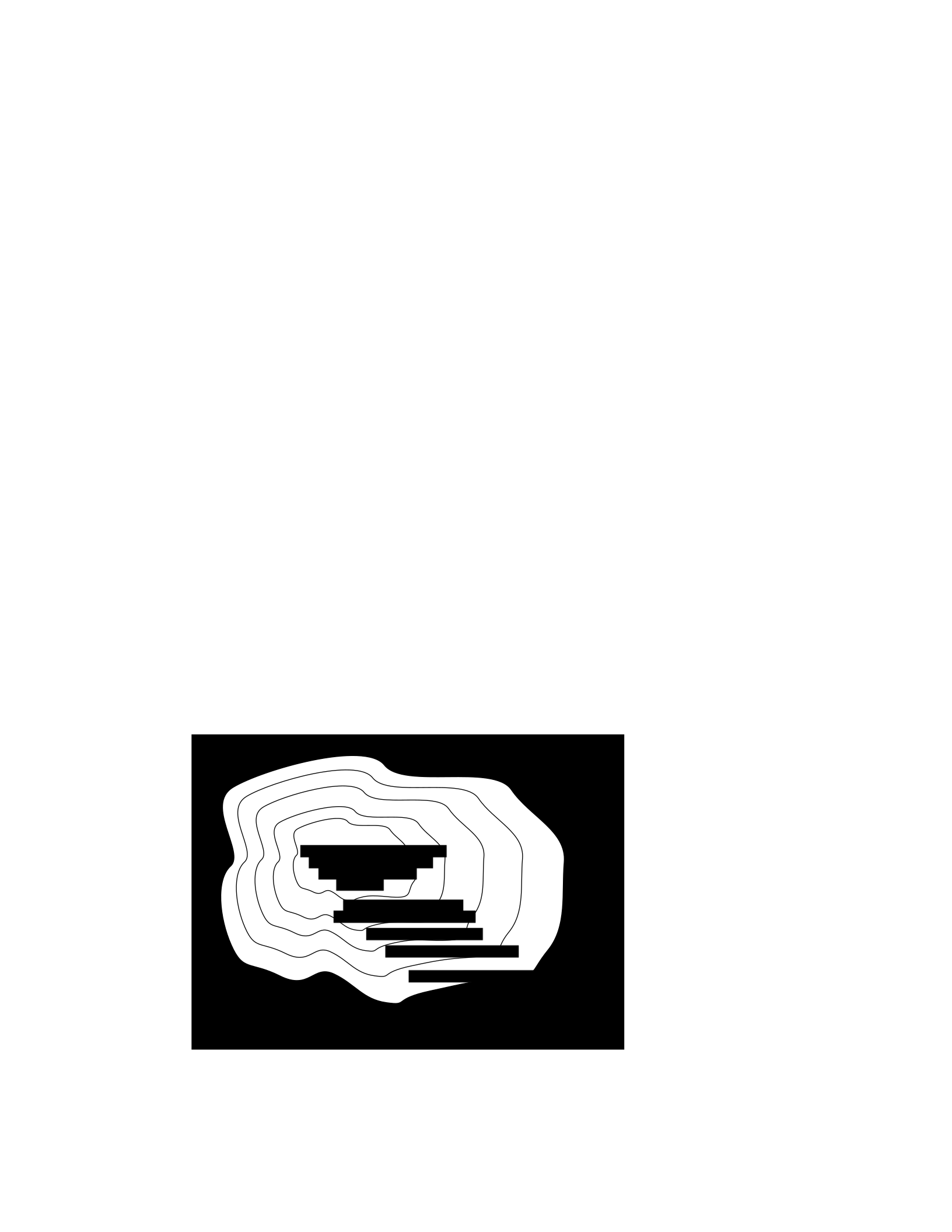
than having to re-invent the techniques yourself. And other people will be able to readily understand and
modify your designs.
We can often make a design job easier by limiting the space of possible designs, and by standardizing on:
• a basis set of primitive components;
• ways of combining the primitive components to make more complex systems;
• ways of “packaging” or abstracting pieces of a design so they can be reused (in essence creating
new “primitives”); and
• ways of capturing common patterns of abstraction (essentially, abstracting our abstractions).
Very complicated design problems can become tractable using such a primitive-combinationabstraction-
pattern (PCAP) approach. In this class, we will examine and learn to use a variety of PCAP strategies
common in EE and CS, and will even design some of our own, for special purposes. In the rest of this
section, we will hint at some of the PCAP systems we will be developing in much greater depth throughout
the class. Figure 1.1 shows one view of this development, as a successive set of restrictions of the design
space of mechanisms.
One very important thing about abstract models is that once we have fixed the abstraction, it will usually
be possible to implement it using a variety of different underlying substrates. So, as shown in figure 1.2,
we can construct general-purpose computers out of a variety of different kinds of systems, including digital
circuits and general-purpose computers. And systems satisfying the digital circuit abstraction can be
constructed from analog circuits, but also from gears or water or light.
Another demonstration of the value of abstracted models is that we can use them, by analogy, to describe
quite different systems. So, for example, the constraint models of circuits that we will study can be applied
to describing transmission of neural signals down the spinal cord, or of heat through a network of
connected bodies.
Let’s explore the abstraction hierarchy figure 1.1 in some more detail, moving up abstraction levels while
observing common patterns.
Figure 1.1 Increasingly constrained systems.
electrical systems
traditional analog circuits
digital electronic circuits
electronic computers
electronic computers
running Python programs
electronic computers with
Python programs that
select outputs by
planning

Figure 1.2 A single abstraction may have a variety of different underlying implementations.
Circuits
Typical electronics circuits are built out of a basis set of primitive components such as voltage sources,
resistors, capacitors, inductors and transistors. This set of component types was chosen to be closely
related to primitive concepts in our physical understanding of electronic systems in terms of voltage,
current, resistance, and the rate of change of those quantities over time. So, when we buy a physical
resistor, we tend to think only of its resistance; and when we buy a capacitor, we think of its ability to store
charge. But, of course, that physical resistor has some capacitance, and the capacitor, some resistance.
Still, it helps us in our designs to have devices that are as close to the ideal models as possible; and it helps
that people have been designing with these components for years, so that we can adopt the strategies
that generations of clever people have developed.
The method of combining circuit elements is to connect their terminals with conductors (wires, crimps,
solder, etc.), a process that is generically referred to as wiring. And our method of abstraction is to describe
the constraints that a circuit element exerts on the currents and voltages of terminals to which the
element is connected.
So, armed with the standard basis set of analog circuit components, we can try to build a circuit to control
our robot. We have a resistance that varies with the light level, but we need a voltage that does so, as well.
We can achieve this by using a voltage divider, which is shown in figure 1.3A. Using an abstract, constraint-
based model of the behavior of circuit components that we will
General-purpose computer
Digital circuits
T
uring
machine
Cellular
automata
Analog
electronics
Gears
Light
W
ater

study in detail later in the course, we can determine the following relationship between Vout and
Vin:
RB
Vout = Vin .
RA + RB
So, for example, if RA = RB, then Vout = Vin/2. Or, in our case, if RA actually varies with the amount
of light shining on it, then Vout will also vary with the light.
13
Vin Vin Vin
RARARA
Vout
RBRBmotor RBmotor
Figure 1.3 Voltage dividers: A. Resistor divider. B. Connected to a motor, in a way that breaks
the abstraction from part A. C. Connected to a motor, with a buffer.
That is great. So, now, we might imagine that we could use this voltage difference that we have
created to drive the motor at different speeds, depending on the light hitting the resistor, using
a circuit something like the one shown in figure 1.3B. But, sadly, that will not work. It turns out
that once we connect the motor to the circuit, it actually changes the voltages, and we can no
longer maintain the voltage difference needed to drive the motor.
So, although we have developed an abstract model of the behavior of circuit components, which
lets us analyze the behavior of a particular complete circuit design, it does not give us
modularity. That is, we cannot design two parts of a circuit, understand each of their behaviors,
and then predict the behavior of the composite system based on the behavior of the separate
components. Instead, we would have to re-analyze the joint behavior of the whole composite
system. Lack of modularity makes it very difficult to design large systems, because two different
people, or the same person at two different times, cannot design pieces and put them together
without understanding the whole.
To solve this problem, we can augment our analog-circuit toolbox with some additional
components that allow us to design components with modular behavior; they “buffer” or
“isolate” one part of the circuit from another in ways that allow us to combine the parts more
13
Do not worry if this example does not make much sense to you; we will explore this all in great detail later.

easily. In this class, we will use op-amps to build buffers, which will let us solve our sample
problem using a slightly more complex circuit, as shown in figure 1.3C.
Thus, the key point is that good modules preserve abstraction barriers between the use of a
module and internal details of how they are constructed. We will see this theme recur as we
discuss different PCAP systems.
Digital circuits
In analog circuits, we think about voltages on terminals ranging over real values. This gives us
the freedom to create an enormous variety of circuits, but sometimes that freedom actually
makes the design process more difficult. To design ever more complex circuits, we can move to
a much stronger, digital abstraction, in which the voltages on the terminals are thought of as
only taking on values that are either “low” or “high” (often called 0 and 1). This PCAP system is
made up of a basis set of elements, called gates, that are built out of simpler analog circuit
components, such as transistors and resistors. Adopting the digital abstraction is a huge
limitation on the kinds of circuits that can be built. However, digital circuits can be easy to design
and build and also can be inexpensive because the basic elements (gates) are simple (fewer
transisters are need to construct a gate than to construct an op amp), versatile (only a small
number of different kinds of logic elements are necessary to construct an arbitrary digital
circuit), and combinations are easy to think about (using Boolean logic). These properties allow
designers to build incredibly complex machines by designing small parts and putting them
together into increasingly larger pieces. Digital watches, calculators, and computers are all built
this way.
Digital design is a very important part of EECS, and it is treated in a number of our courses at
basic and advanced levels, but is not one of the topics we will go into in detail in 6.01.
Nevertheless, the same central points that we explore in this course apply to this domain as
well.
Computers
One of the most important developments in the design of digital circuits is that of the
generalpurpose “stored program” computer. Computers are a particular class of digital circuits
that are general purpose: the same actual circuit can perform (almost) any transformation
between its inputs and its outputs. Which particular transformation it performs is governed by
a program, which is some settings of physical switches, or information written on an external
physical memory, such as cards or a tape, or information stored in some sort of internal memory.
The “almost” in the previous section refers to the actual memory capacity of the computer.
Exactly what computations a computer can perform depends on the amount of memory it has;
and also on the time you are willing to wait. So, although a general-purpose computer can do
anything a special-purpose digital circuit can do, in the information-processing sense, the
computer might be slower or use more power. However, using general-purpose computers can
save an enormous amount of engineering time and effort. It is much cheaper and easier to
debug and modify and manufacture software than hardware. The modularities and abstractions
that software PCAP systems give us are even more powerful than those derived from the digital
circuit abstraction.

Again, we can see how abstraction separates use from details; we don’t need to know how the
circuits inside a computer are designed, we just need to know the rules by which we can use
them and the constraints under which they perform.
Python programs
Every general-purpose computer has a different detailed design, which means that the way its
program needs to be specified is different. Furthermore, the “machine languages” for
describing computer programs, at the most primitive level, are awkward for human
programmers. So, we have developed a number of computer programming languages for
specifying a desired computation. These languages are converted into instructions in the
computer’s native machine language by other computer programs, called compilers or
interpreters. One of the coolest and most powerful things about general-purpose computers is
this ability to write computer programs that process or create or modify other computer
programs.
Computer programming languages are PCAP systems. They provide primitive operations, ways
of combining them, ways of abstracting over them, and ways of capturing common abstraction
patterns. We will spend a considerable amount of time in this course studying the particular
primitives, combination mechanisms, and abstraction mechanisms made available in the
Python programming language. But the choice of Python is relatively unimportant. Virtually all
modern programming languages supply a similar set of mechanisms, and the choice of
programming language is primarily a matter of taste and convenience.
In a computer program we have both data primitives and computation primitives. At the most
basic level, computers generally store binary digits (bits) in groups of 32 or 64, called words.
These words are data primitives, and they can be interpreted by our programs as representing
integers, floating-point numbers, strings, or addresses of other data in the computer’s memory.
The computational primitives supported by most computers include numerical operations such
as addition and multiplication, and locating and extracting the contents of a memory at a given
address. In Python, we will work at a level of abstraction that does not require us to think very
much about addresses of data, but it is useful to understand that level of description, as well.
Primitive data and computation elements can be combined and abstracted in a variety of
different ways, depending on choices of programming style. We will explore these in more detail
in section 1.3.2.
1.2.3 Models
So far, we have discussed a number of ways of framing the problem of designing and
constructing mechanisms. Each PCAP system is accompanied by a modeling system that lets us
make mathematical models of the systems we construct.
What is a model? It is a new system that is considerably simpler than the system being modeled,
but which captures the important aspects of the original system. We might make a physical
model of an airplane to test in a wind tunnel. It does not have to have passenger seats or landing
lights; but it has to have surfaces of the correct shape, in order to capture the important
properties for this purpose. Mathematical models can capture properties of systems that are

important to us, and allow us to discover things about the system much more conveniently than
by manipulating the original system itself.
One of the hardest things about building models is deciding which aspects of the original system
to model and which ones to ignore. Many classic, dramatic engineering failures can be ascribed
to failing to model important aspects of the system. One example (which turned out to be an
ethical success story, rather than a failure) is LeMessurier’s Citicorp Building
14
, in which an
engineering design change was made, but tested in a model in which the wind came only from
a limited set of directions.
Another important dimension in modeling is whether the model is deterministic or not. We
might, for example, model the effect of the robot executing a command to set its velocity as
making an instantaneous change to the commanded velocity. But, of course, there is likely to
be some delay and some error. We have to decide whether to ignore that delay and error in our
model and treat it as if it were ideal; or, for example, to make a probabilistic model of the
possible results of that command. Generally speaking, the more different the possible outcomes
of a particular action or command, and the more diffuse the probability distribution over those
outcomes, the more important it is to explicitly include uncertainty in the model.
Once we have a model, we can use it in a variety of different ways, which we explore below.
Analytical models
By far the most prevalent use of models is in analysis: Given a circuit design, what will the
voltage on this terminal be? Given a computer program, will it compute the desired answer?
How long will it take? Given a control system, implemented as a circuit or as a program, will the
system stop at the right distance from the light bulb?
Analytical tools are important. It can be hard to verify the correctness of a system by trying it in
all possible initial conditions with all possible inputs; sometimes it is easier to develop a
mathematical model and then prove a theorem about the model.
For some systems, such as pure software computations, or the addition circuitry in a calculator,
it is possible to analyze correctness or speed with just a model of the system in question. For
other systems, such as fuel injectors, it is impossible to analyze the correctness of the controller
without also modeling the environment (or “plant”) to which it is connected, and then analyzing
the behavior of the coupled system of the controller and environment.
To demonstrate some of these tradeoffs, we can do a very simple analysis of a robot moving
toward a lamp. Imagine that we arrange it so that the robot’s velocity at time t, V[t], is
proportional to the difference between the actual light level, X[t], and a desired light level (that
is, the light level we expect to encounter when the robot is the desired distance from the lamp),
Xdesired ; that is, we can model our control system with the difference equation
14
See “The Fifty-Nine Story Crisis”, The New Yorker, May 29, 1995, pp 45-53.

V[t] = k(Xdesired − X[t]) where k is the constant of
proportionality, or gain, of the controller.
Now, we need to model the world. For simplicity, we equate the light level to the robot’s position
(assuming that the units match); in addition we assume the robot’s position at time t is its
position at time t−1 plus its velocity at time t−1 (actually, this should be the product of the
velocity and the length of time between samples, but we can just assume a unit time step and
thus use velocity). When we couple these models, we get the difference equation
X[t] = X[t − 1] + k(Xdesired − X[t − 1]) .
Now, for a given value of k, we can determine how the system will behave over time, by solving
the difference equation in X.
Later in the course, we will see how easily-determined mathematical properties of a
differenceequation model can tell us whether a control system will have the desired behavior
and whether or not the controller will cause the system to oscillate. These same kinds of
analyses can be applied to robot control systems as well as to the temporal properties of
voltages in a circuit, and even to problems as unrelated as the consequences of a monetary
policy decision in economics. It is important to note that treating the system as moving in
discrete time steps is an approximation to underlying continuous dynamics; it can make models
that are easier to analyze, but it requires sophisticated understanding of sampling to understand
the effects of this approximation on the correctness of the results.
Synthetic models
One goal of many people in a variety of sub-disciplines of computer science and electrical
engineering is automatic synthesis of systems from formal descriptions of their desired
behavior. For example, you might describe some properties you would want the input/output
behavior of a circuit or computer program to have, and then have a computer system discover
a circuit or program with the desired property.
This is a well-specified problem, but generally the search space of possible circuits or programs
is much too large for an automated process; the intuition and previous experience of an expert
human designer cannot yet be matched by computational search methods.
However, humans use informal models of systems for synthesis. The documentation of a
software library, which describes the function of the various procedures, serves as an informal
model that a programmer can use to assemble those components to build new, complex
systems.
Internal models
As we wish to build more and more complex systems with software programs as controllers, we
find that it is often useful to build additional layers of abstraction on top of the one provided by
a generic programming language. This is particularly true when the nature of the exact

computation required depends considerably on information that is only received during the
execution of the system.
Consider, for example, an automated taxi robot (or, more prosaically, the navigation system in
your new car). It takes, as input, a current location in the city and a goal location, and gives, as
output, a path from the current location to the goal. It has a map built into it.
It is theoretically possible to build an enormous digital circuit or computer program that
contains a look-up table, in which we precompute the path for all pairs of locations and store
them away. Then when we want to find a path, we could simply look in the table at the location
corresponding to the start and goal location and retrieve the precomputed path. Unfortunately,
the size of that table is too huge to contemplate. Instead, what we do is construct an abstraction
of the problem as one of finding a path from any start state to any goal state, through a graph
(an abstract mathematical construct of “nodes” with “arcs” connecting them). We can develop
and implement a general-purpose algorithm that will solve any shortest-path problem in a
graph. That algorithm and implementation will be useful for a wide variety of possible problems.
And for the navigation system, all we have to do is represent the map as a graph, specify the
start and goal states, and call the general graph-search algorithm.
We can think of this process as actually putting a model of the system’s interactions with the
world inside the controller; it can consider different courses of action in the world and pick the
one that is the best according to some criterion.
Another example of using internal models is when the system has some significant lack of
information about the state of the environment. In such situations, it may be appropriate to
explicitly model the set of possible states of the external world and their associated
probabilities, and to update this model over time as new evidence is gathered. We will pursue
an example of this approach near the end of the course.
1.3 Programming embedded systems
There are many different ways of thinking about modularity and abstraction for software.
Different models will make some things easier to say and do and others more difficult, making
different models appropriate for different tasks. In the following sections, we explore different
strategies for building software systems that interact with an external environment, and then
different strategies for specifying the purely computational part of a system.
1.3.1 Interacting with the environment
Increasingly, computer systems need to interact with the world around them, receiving
information about the external world, and taking actions to affect the world. Furthermore, the
world is dynamic, so that as the system is computing, the world is changing, requiring future
computation to adapt to the new state of the world.
There are a variety of different ways to organize computations that interact with an external
world. Generally speaking, such a computation needs to:
19. get information from sensors (light sensors, sonars, mouse, keyboard, etc.),
20. perform computation, remembering some of the results, and

21. take actions to change the outside world (move the robot, print, draw, etc.).
These operations can be put together in different styles.
1.3.1.1 Sequential
The most immediately straightforward style for constructing a program that interacts with the
world is the basic imperative style, in which the program gives a sequence of ’commands’ to the
system it is controlling. A library of special procedures is defined, some of which read
information from the sensors and others of which cause actions to be performed. Example
procedures might move a robot forward a fixed distance, or send a file out over the network, or
move video-game characters on the screen.
In this model, we could naturally write a program that moves an idealized robot in a square, if
there is space in front of it.
if noObstacleInFront:
moveDistance(1)
turnAngle(90)
moveDistance(1)
turnAngle(90)
moveDistance(1)
turnAngle(90)
moveDistance(1)
turnAngle(90)
The major problem with this style of programming is that the programmer has to remember to
check the sensors sufficiently frequently. For instance, if the robot checks for free space in front,
and then starts moving, it might turn out that a subsequent sensor reading will show that there
is something in front of the robot, either because someone walked in front of it or because the
previous reading was erroneous. It is hard to have the discipline, as a programmer, to remember
to keep checking the sensor conditions frequently enough, and the resulting programs can be
quite difficult to read and understand.
For the robot moving toward the light, we might write a program like this:
while lightValue <
desiredValue:
moveDistance(0.1)
This would have the robot creep up, step by step, toward the light. We might want to modify it
so that the robot moved a distance that was related to the difference between the current and
desired light values. However, if it takes larger steps, then during the time that it is moving it
will not be sensitive to possible changes in the light value and cannot react immediately to
them.
1.3.1.2 Event-Driven
User-interface programs are often best organized differently, as event-driven (also called
interrupt driven) programs. In this case, the program is specified as a collection of procedures

(called ’handlers’ or ’callbacks’) that are attached to particular events that can take place. So,
for example, there might be procedures that are called when the mouse is clicked on each
button in the interface, when the user types into a text field, or when the temperature of a
reactor gets too high. An “event loop” runs continuously, checking to see whether any of the
triggering events have happened, and, if they have, calling the associated procedure.
In our simple example, we might imagine writing a program that told the robot to drive forward
by default; and then install an event handler that says that if the light level reaches the desired
value, it should stop. This program would be reactive to sudden changes in the environment.
As the number and frequency of the conditions that need responses increases, it can be difficult
to both keep a program like this running well and guarantee a minimum response time to any
event.
1.3.1.3 Transducer
An alternative view is that programming a system that interacts with an external world is like
building a transducer with internal state. Think of a transducer as a processing box that runs
continuously. At regular intervals (perhaps many times per second), the transducer reads all of
the sensors, does a small amount of computation, stores some values it will need for the next
computation, and then generates output values for the actions.
This computation happens over and over and over again. Complex behavior can arise out of the
temporal pattern of inputs and outputs. So, for example, a robot might try to move forward
without hitting something by defining a procedure:
def step(): distToFront = min(frontSonarReadings)
motorOutput(gain * (distToFront - desiredDistance), 0.0)
Executed repeatedly, this program will automatically modulate the robot’s speed to be
proportional to the free space in front of it.
The main problem with the transducer approach is that it can be difficult to do tasks that are
fundamentally sequential (like the example of driving in a square, shown above). We will start
with the transducer model, and then, as described in section 4.3, we will build a new abstraction
layer on top of it that will make it easy to do sequential commands, as well.
1.3.2 Programming models
Just as there are different strategies for organizing entire software systems, there are different
strategies for formally expressing computational processes within those structures.
1.3.2.1 Imperative computation
Most of you have probably been exposed to an imperative model of computer programming, in
which we think of programs as giving a sequential set of instructions to the computer to do
something. And, in fact, that is how the internals of the processors of computers are typically
structured. So, in Java or C or C++, you write typically procedures that consist of lists of
instructions to the computer:

25. Put this value in this variable
26. Square the variable
27. Divide it by pi
28. If the result is greater than 1, return the result
In this model of computation, the primitive computational elements are basic arithmetic
operations and assignment statements. We can combine the elements using sequences of
statements, and control structures such as if, for, and while. We can abstract away from the
details of a computation by defining a procedure that does it. Now, the engineer only needs to
know the specifications of the procedure, but not the implementation details, in order to use
it.
1.3.2.2 Functional computation
Another style of programming is the functional style. In this model, we gain power through
function calls. Rather than telling the computer to do things, we ask it questions: What is 4 + 5?
What is the square root of 6? What is the largest element of the list?
These questions can all be expressed as asking for the value of a function applied to some
arguments. But where do the functions come from? The answer is, from other functions. We
start with some set of basic functions (like “plus”), and use them to construct more complex
functions.
This method would not be powerful without the mechanisms of conditional evaluation and
recursion. Conditional functions ask one question under some conditions and another question
under other conditions. Recursion is a mechanism that lets the definition of a function refer to
the function being defined. Recursion is as powerful as iteration.
In this model of computation, the primitive computational elements are typically basic
arithmetic and list operations. We combine elements using function composition (using the
output of one function as the input to another), if, and recursion. We use function definition as
a method of abstraction, and the idea of higher-order functions (passing functions as arguments
to other functions) as a way of capturing common high-level patterns.
1.3.2.3 Data structures
In either style of asking the computer to do work for us, we have another kind of modularity
and abstraction, which is centered around the organization of data.
At the most primitive level, computers operate on collections of (usually 32 or 64) bits. We can
interpret such a collection of bits as representing different things: a positive integer, a signed
integer, a floating-point number, a Boolean value (true or false), one or more characters, or an
address of some other data in the memory of the computer. Python gives us the ability to work
directly with all of these primitives, except for addresses.
There is only so much you can do with a single number, though. We would like to build computer
programs that operate on representations of documents or maps or circuits or social networks.

To do so, we need to aggregate primitive data elements into more complex data structures.
These can include lists, arrays, dictionaries, and other structures of our own devising.
Here, again, we gain the power of abstraction. We can write programs that do operations on a
data structure representing a social network, for example, without having to worry about the
details of how the social network is represented in terms of bits in the machine.
1.3.2.4 Object-oriented programming: computation + data structures
Object-oriented programming is a style that applies the ideas of modularity and abstraction to
execution and data at the same time.
An object is a data structure, together with a set of procedures that operate on the data. Basic
procedures can be written in an imperative or a functional style, but ultimately there is
imperative assignment to state variables in the object.
One major new type of abstraction in OO programming is “generic” programming. It might be
that all objects have a procedure called print associated with them. So, we can ask any object
to print itself, without having to know how it is implemented. Or, in a graphics system, we might
have a variety of different objects that know their x,y positions on the screen. So each of them
can be asked, in the same way, to say what their position is, even though they might be
represented very differently inside the objects.
In addition, most object-oriented systems support inheritance, which is a way to make new
kinds of objects by saying that they are mostly like another kind of object, but with some
exceptions.
This is another way to take advantage of abstraction.
Programming languages
Python as well as other modern programming languages, such as Java, Ruby and C++, support
all of these programming models. The programmer needs to choose which programming model
best suits the task. This is an issue that we will return to throughout the course.
1.4 Summary
We hope that this course will give you a rich set of conceptual tools and practical techniques,
as well as an appreciation of how math, modeling, and implementation can work together to
enable the design and analysis of complex computational systems that interact with the world.
Acknowledgments
Thanks to Jacob White, Hal Abelson, Tomas Lozano-Perez, Sarah Finney, Sari Canelake, Eric
Grimson, Ike Chuang, and Berthold Horn for useful comments and criticisms, and to Denny
Freeman for significant parts and most of the figures in the linear systems chapter. - LPK
1.1 Goals for 6.01
We have many goals for this course. Our primary goal is for you to learn to appreciate and use the
fundamental design principles of modularity and abstraction in a variety of contexts from electrical

engineering and computer science. To achieve this goal, we will study electrical engineering (EE) and
computer science (CS) largely from the perspective of how to build systems that interact with, and attempt
to control, an external environment. Such systems include everything from low-level controllers like heat
regulators or cardiac pacemakers, to medium-level systems like automated navigation or virtual surgery,
to high-level systems that provide more natural human-computer interfaces.
Our second goal is to show you that making mathematical models of real systems can help in the design
and analysis of those systems; and to give you practice with the difficult step of deciding which aspects of
the real world are important to the problem being solved and how to model them in ways that give insight
into the problem.
We also hope to engage you more actively in the educational process. Most of the work of this course will
not be like typical problems from the end of a chapter. You will work individually and in pairs to solve
problems that are deeper and more open-ended. There will not be a unique right answer. Argument,
explanation, and justification of approach will be more important than the answer. We hope to expose
you to the ubiquity of trade-offs in engineering design: it is rare that an approach will be best in every
dimension; some will excel in one way, others in a different way. Deciding how to make such trade-offs is
a crucial part of engineering.
Another way in which we hope to engage you in the material is by having many of you return to the course
as lab assistants in future semesters. Having a large number of lab assistants in the class means that
students can be given more open-ended problems, and have people around to help them when they are
stuck. Even more importantly, the lab assistants are meant to question the students as they go; to
challenge their understanding and help them see and evaluate a variety of approaches. This process is of
great intellectual value to student and lab assistant alike.
Finally, of course, we have the more typical goals of teaching exciting and important basic material from
electrical engineering and computer science, including modern software engineering, linear systems
analysis, electronic circuits, and decision-making. This material all has an internal elegance and beauty, as
well as crucial role in building modern EE and CS systems.
1.2 Modularity, abstraction, and modeling
Whether proving a theorem by building up from lemmas to basic theorems to more specialized results, or
designing a circuit by building up from components to modules to complex processors, or designing a
software system by building up from generic procedures to classes to class libraries, humans deal with
complexity by exploiting the power of abstraction and modularity. Without such tools, a single person
would be overwhelmed by the complexity of a system, as there is only so much detail that a single person
can consciously manage at a time.
Modularity is the idea of building components that can be re-used; and abstraction is the idea that after
constructing a module (be it software or circuits or gears), most of the details of the module construction
can be ignored and a simpler description used for module interaction (the module computes the square
root, or doubles the voltage, or changes the direction of motion).
Given basic modules, one can move up a level of abstraction and construct a new module by putting
together several previously-built modules, thinking only of their abstract descriptions, and not their
implementations. And, of course, this process can be repeated over many stages. This process gives one

the ability to construct systems with complexity far beyond what would be possible if it were necessary to
understand each component in detail.
Any module can be described in a large number of ways. We might describe the circuitry in a digital watch
in terms of how it behaves as a clock and a stopwatch, or in terms of voltages and currents within the
circuit, or in terms of the heat produced at different parts of the circuitry. Each of these is a different model
of the watch. Different models will be appropriate for different tasks: there is no single correct model.
Rather, each model exposes different dimensions of the system, allowing us to explore many aspects of
the design space of a system, and to trade off different factors in the performance of a system.
The primary theme of this course will be to learn about different methods for building modules out of
primitives, and of building different abstract models of them, so that we can analyze or predict their
behavior, and so we can recombine them into even more complex systems. The same fundamental
principles will apply to software, to control systems, and to circuits.
1.2.1 Example problem
Imagine that you need to make a robot that will roll up close to a light bulb and stop a fixed distance from
it. The first question is, how can we get electrical signals to relate to the physical phenomena of light
readings and robot wheel rotations? There is a large part of electrical engineering related to the design of
physical devices that connect to the physical world in such a way that some electrical property of the
device relates to a physical process in the world. For example, a light-sensitive resistor (photo-resistor) is
a sensor whose resistance changes depending on light intensity impinging on it; a motor is an effector
whose rotor speed is related to the voltage across its two terminals. In this course, we will not examine
the detailed physics of sensors and effectors, but will concentrate on ways of designing systems that use
sensors and effectors to perform both simple and more complicated tasks. To get a robot to stop in front
of a light bulb, the problem will be to find a way to connect the photo-resistor to the motor, so that the
robot will stop at an appropriate distance from the bulb. Thus, we will already use the idea of abstraction
to treat sensors Chapter 1 Course Overview
and effectors as primitive modules whose internal details we can ignore, and whose performance
characteristics we can use as we design systems built on these elements.
1.2.2 An abstraction hierarchy of mechanisms
Given the light-sensitive resistor and the motor, we could find many ways of connecting them, using bits
of metal and ceramic of different kinds, or making some kind of magnetic or mechanical linkages. The
space of possible designs of machines is enormous.
One of the most important things that engineers do, when faced with a set of design problems, is to
standardize on a basis set of components to use to build their systems. There are many reasons for
standardizing on a basis set of components, mostly having to do with efficiency of understanding and of
manufacturing. It is important, as a designer, to develop a repertoire of standard bits and pieces of designs
that you understand well and can put together in various ways to make more complex systems. If you use
the same basis set of components as other designers, you can learn valuable techniques from them, rather
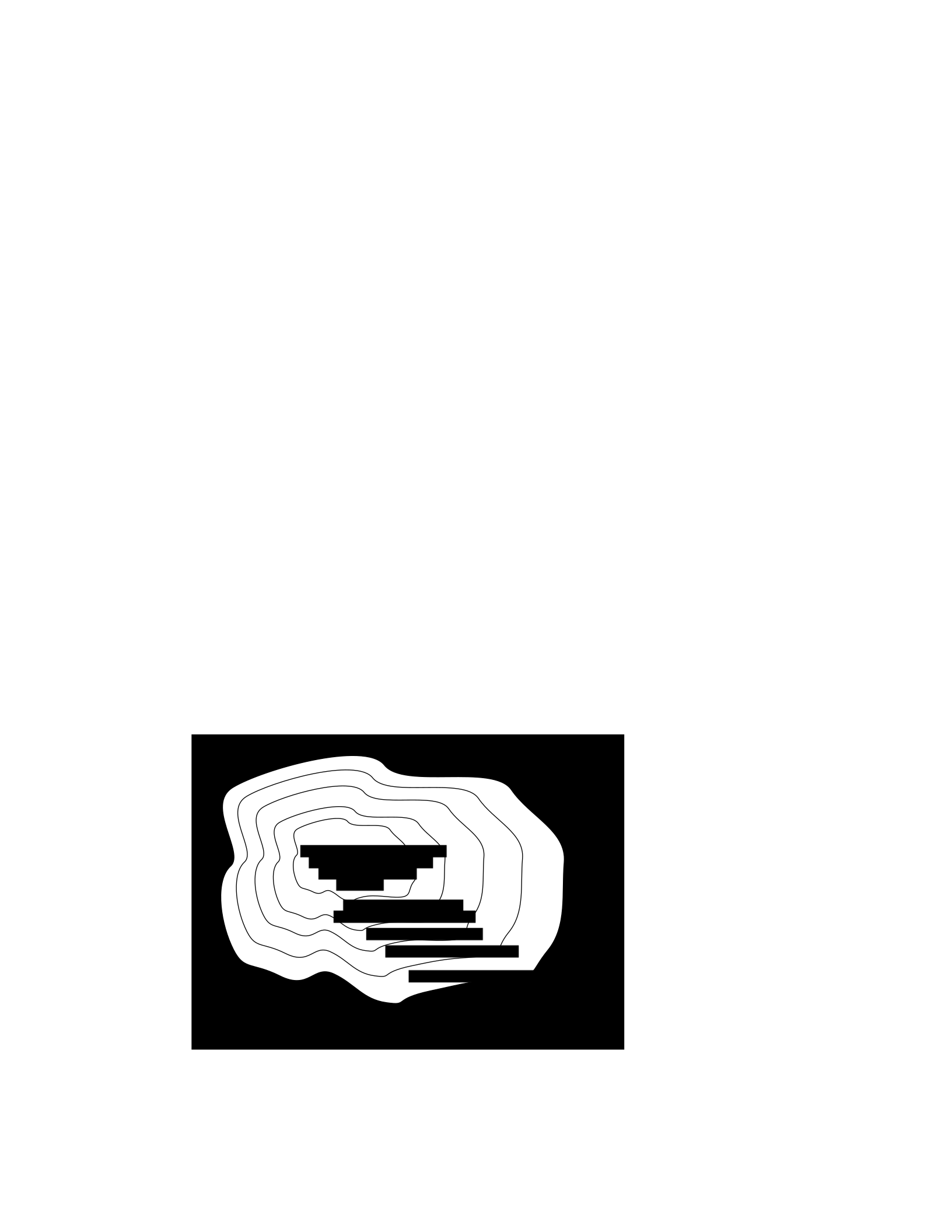
than having to re-invent the techniques yourself. And other people will be able to readily understand and
modify your designs.
We can often make a design job easier by limiting the space of possible designs, and by standardizing on:
• a basis set of primitive components;
• ways of combining the primitive components to make more complex systems;
• ways of “packaging” or abstracting pieces of a design so they can be reused (in essence creating
new “primitives”); and
• ways of capturing common patterns of abstraction (essentially, abstracting our abstractions).
Very complicated design problems can become tractable using such a primitive-combinationabstraction-
pattern (PCAP) approach. In this class, we will examine and learn to use a variety of PCAP strategies
common in EE and CS, and will even design some of our own, for special purposes. In the rest of this
section, we will hint at some of the PCAP systems we will be developing in much greater depth throughout
the class. Figure 1.1 shows one view of this development, as a successive set of restrictions of the design
space of mechanisms.
One very important thing about abstract models is that once we have fixed the abstraction, it will usually
be possible to implement it using a variety of different underlying substrates. So, as shown in figure 1.2,
we can construct general-purpose computers out of a variety of different kinds of systems, including digital
circuits and general-purpose computers. And systems satisfying the digital circuit abstraction can be
constructed from analog circuits, but also from gears or water or light.
Another demonstration of the value of abstracted models is that we can use them, by analogy, to describe
quite different systems. So, for example, the constraint models of circuits that we will study can be applied
to describing transmission of neural signals down the spinal cord, or of heat through a network of
connected bodies.
Let’s explore the abstraction hierarchy figure 1.1 in some more detail, moving up abstraction levels while
observing common patterns.
Figure 1.1 Increasingly constrained systems.
electrical systems
traditional analog circuits
digital electronic circuits
electronic computers
electronic computers
running Python programs
electronic computers with
Python programs that
select outputs by
planning

Figure 1.2 A single abstraction may have a variety of different underlying implementations.
Circuits
Typical electronics circuits are built out of a basis set of primitive components such as voltage sources,
resistors, capacitors, inductors and transistors. This set of component types was chosen to be closely
related to primitive concepts in our physical understanding of electronic systems in terms of voltage,
current, resistance, and the rate of change of those quantities over time. So, when we buy a physical
resistor, we tend to think only of its resistance; and when we buy a capacitor, we think of its ability to store
charge. But, of course, that physical resistor has some capacitance, and the capacitor, some resistance.
Still, it helps us in our designs to have devices that are as close to the ideal models as possible; and it helps
that people have been designing with these components for years, so that we can adopt the strategies
that generations of clever people have developed.
The method of combining circuit elements is to connect their terminals with conductors (wires, crimps,
solder, etc.), a process that is generically referred to as wiring. And our method of abstraction is to describe
the constraints that a circuit element exerts on the currents and voltages of terminals to which the
element is connected.
So, armed with the standard basis set of analog circuit components, we can try to build a circuit to control
our robot. We have a resistance that varies with the light level, but we need a voltage that does so, as well.
We can achieve this by using a voltage divider, which is shown in figure 1.3A. Using an abstract, constraint-
based model of the behavior of circuit components that we will
General-purpose computer
Digital circuits
T
uring
machine
Cellular
automata
Analog
electronics
Gears
Light
W
ater
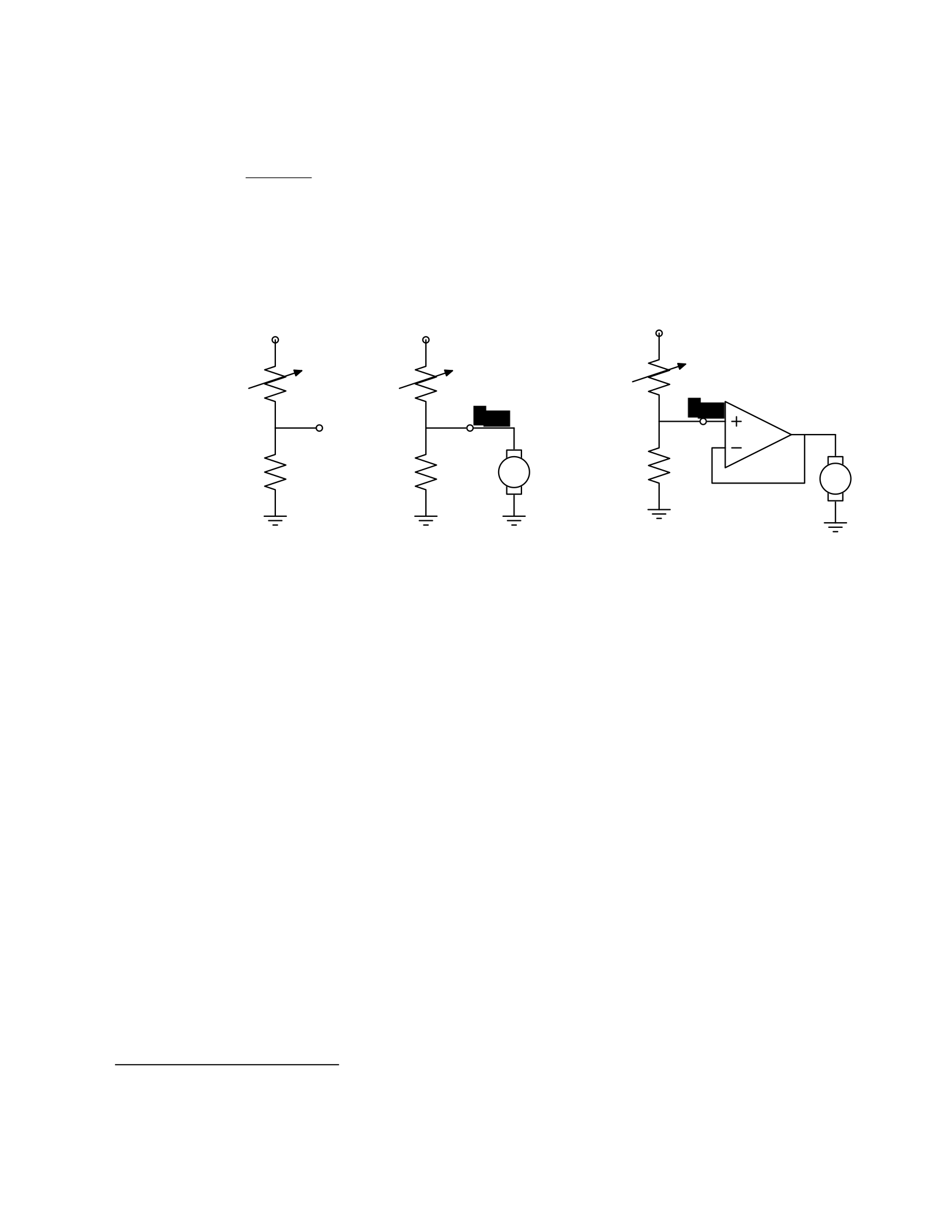
study in detail later in the course, we can determine the following relationship between Vout and
Vin:
RB
Vout = Vin .
RA + RB
So, for example, if RA = RB, then Vout = Vin/2. Or, in our case, if RA actually varies with the amount
of light shining on it, then Vout will also vary with the light.
15
Vin Vin Vin
RARARA
Vout
RBRBmotor RBmotor
Figure 1.3 Voltage dividers: A. Resistor divider. B. Connected to a motor, in a way that breaks
the abstraction from part A. C. Connected to a motor, with a buffer.
That is great. So, now, we might imagine that we could use this voltage difference that we have
created to drive the motor at different speeds, depending on the light hitting the resistor, using
a circuit something like the one shown in figure 1.3B. But, sadly, that will not work. It turns out
that once we connect the motor to the circuit, it actually changes the voltages, and we can no
longer maintain the voltage difference needed to drive the motor.
So, although we have developed an abstract model of the behavior of circuit components, which
lets us analyze the behavior of a particular complete circuit design, it does not give us
modularity. That is, we cannot design two parts of a circuit, understand each of their behaviors,
and then predict the behavior of the composite system based on the behavior of the separate
components. Instead, we would have to re-analyze the joint behavior of the whole composite
system. Lack of modularity makes it very difficult to design large systems, because two different
people, or the same person at two different times, cannot design pieces and put them together
without understanding the whole.
To solve this problem, we can augment our analog-circuit toolbox with some additional
components that allow us to design components with modular behavior; they “buffer” or
“isolate” one part of the circuit from another in ways that allow us to combine the parts more
15
Do not worry if this example does not make much sense to you; we will explore this all in great detail later.

easily. In this class, we will use op-amps to build buffers, which will let us solve our sample
problem using a slightly more complex circuit, as shown in figure 1.3C.
Thus, the key point is that good modules preserve abstraction barriers between the use of a
module and internal details of how they are constructed. We will see this theme recur as we
discuss different PCAP systems.
Digital circuits
In analog circuits, we think about voltages on terminals ranging over real values. This gives us
the freedom to create an enormous variety of circuits, but sometimes that freedom actually
makes the design process more difficult. To design ever more complex circuits, we can move to
a much stronger, digital abstraction, in which the voltages on the terminals are thought of as
only taking on values that are either “low” or “high” (often called 0 and 1). This PCAP system is
made up of a basis set of elements, called gates, that are built out of simpler analog circuit
components, such as transistors and resistors. Adopting the digital abstraction is a huge
limitation on the kinds of circuits that can be built. However, digital circuits can be easy to design
and build and also can be inexpensive because the basic elements (gates) are simple (fewer
transisters are need to construct a gate than to construct an op amp), versatile (only a small
number of different kinds of logic elements are necessary to construct an arbitrary digital
circuit), and combinations are easy to think about (using Boolean logic). These properties allow
designers to build incredibly complex machines by designing small parts and putting them
together into increasingly larger pieces. Digital watches, calculators, and computers are all built
this way.
Digital design is a very important part of EECS, and it is treated in a number of our courses at
basic and advanced levels, but is not one of the topics we will go into in detail in 6.01.
Nevertheless, the same central points that we explore in this course apply to this domain as
well.
Computers
One of the most important developments in the design of digital circuits is that of the
generalpurpose “stored program” computer. Computers are a particular class of digital circuits
that are general purpose: the same actual circuit can perform (almost) any transformation
between its inputs and its outputs. Which particular transformation it performs is governed by
a program, which is some settings of physical switches, or information written on an external
physical memory, such as cards or a tape, or information stored in some sort of internal memory.
The “almost” in the previous section refers to the actual memory capacity of the computer.
Exactly what computations a computer can perform depends on the amount of memory it has;
and also on the time you are willing to wait. So, although a general-purpose computer can do
anything a special-purpose digital circuit can do, in the information-processing sense, the
computer might be slower or use more power. However, using general-purpose computers can
save an enormous amount of engineering time and effort. It is much cheaper and easier to
debug and modify and manufacture software than hardware. The modularities and abstractions
that software PCAP systems give us are even more powerful than those derived from the digital
circuit abstraction.

Again, we can see how abstraction separates use from details; we don’t need to know how the
circuits inside a computer are designed, we just need to know the rules by which we can use
them and the constraints under which they perform.
Python programs
Every general-purpose computer has a different detailed design, which means that the way its
program needs to be specified is different. Furthermore, the “machine languages” for
describing computer programs, at the most primitive level, are awkward for human
programmers. So, we have developed a number of computer programming languages for
specifying a desired computation. These languages are converted into instructions in the
computer’s native machine language by other computer programs, called compilers or
interpreters. One of the coolest and most powerful things about general-purpose computers is
this ability to write computer programs that process or create or modify other computer
programs.
Computer programming languages are PCAP systems. They provide primitive operations, ways
of combining them, ways of abstracting over them, and ways of capturing common abstraction
patterns. We will spend a considerable amount of time in this course studying the particular
primitives, combination mechanisms, and abstraction mechanisms made available in the
Python programming language. But the choice of Python is relatively unimportant. Virtually all
modern programming languages supply a similar set of mechanisms, and the choice of
programming language is primarily a matter of taste and convenience.
In a computer program we have both data primitives and computation primitives. At the most
basic level, computers generally store binary digits (bits) in groups of 32 or 64, called words.
These words are data primitives, and they can be interpreted by our programs as representing
integers, floating-point numbers, strings, or addresses of other data in the computer’s memory.
The computational primitives supported by most computers include numerical operations such
as addition and multiplication, and locating and extracting the contents of a memory at a given
address. In Python, we will work at a level of abstraction that does not require us to think very
much about addresses of data, but it is useful to understand that level of description, as well.
Primitive data and computation elements can be combined and abstracted in a variety of
different ways, depending on choices of programming style. We will explore these in more detail
in section 1.3.2.
1.2.3 Models
So far, we have discussed a number of ways of framing the problem of designing and
constructing mechanisms. Each PCAP system is accompanied by a modeling system that lets us
make mathematical models of the systems we construct.
What is a model? It is a new system that is considerably simpler than the system being modeled,
but which captures the important aspects of the original system. We might make a physical
model of an airplane to test in a wind tunnel. It does not have to have passenger seats or landing
lights; but it has to have surfaces of the correct shape, in order to capture the important
properties for this purpose. Mathematical models can capture properties of systems that are

important to us, and allow us to discover things about the system much more conveniently than
by manipulating the original system itself.
One of the hardest things about building models is deciding which aspects of the original system
to model and which ones to ignore. Many classic, dramatic engineering failures can be ascribed
to failing to model important aspects of the system. One example (which turned out to be an
ethical success story, rather than a failure) is LeMessurier’s Citicorp Building
16
, in which an
engineering design change was made, but tested in a model in which the wind came only from
a limited set of directions.
Another important dimension in modeling is whether the model is deterministic or not. We
might, for example, model the effect of the robot executing a command to set its velocity as
making an instantaneous change to the commanded velocity. But, of course, there is likely to
be some delay and some error. We have to decide whether to ignore that delay and error in our
model and treat it as if it were ideal; or, for example, to make a probabilistic model of the
possible results of that command. Generally speaking, the more different the possible outcomes
of a particular action or command, and the more diffuse the probability distribution over those
outcomes, the more important it is to explicitly include uncertainty in the model.
Once we have a model, we can use it in a variety of different ways, which we explore below.
Analytical models
By far the most prevalent use of models is in analysis: Given a circuit design, what will the
voltage on this terminal be? Given a computer program, will it compute the desired answer?
How long will it take? Given a control system, implemented as a circuit or as a program, will the
system stop at the right distance from the light bulb?
Analytical tools are important. It can be hard to verify the correctness of a system by trying it in
all possible initial conditions with all possible inputs; sometimes it is easier to develop a
mathematical model and then prove a theorem about the model.
For some systems, such as pure software computations, or the addition circuitry in a calculator,
it is possible to analyze correctness or speed with just a model of the system in question. For
other systems, such as fuel injectors, it is impossible to analyze the correctness of the controller
without also modeling the environment (or “plant”) to which it is connected, and then analyzing
the behavior of the coupled system of the controller and environment.
To demonstrate some of these tradeoffs, we can do a very simple analysis of a robot moving
toward a lamp. Imagine that we arrange it so that the robot’s velocity at time t, V[t], is
proportional to the difference between the actual light level, X[t], and a desired light level (that
is, the light level we expect to encounter when the robot is the desired distance from the lamp),
Xdesired ; that is, we can model our control system with the difference equation
16
See “The Fifty-Nine Story Crisis”, The New Yorker, May 29, 1995, pp 45-53.

V[t] = k(Xdesired − X[t]) where k is the constant of
proportionality, or gain, of the controller.
Now, we need to model the world. For simplicity, we equate the light level to the robot’s position
(assuming that the units match); in addition we assume the robot’s position at time t is its
position at time t−1 plus its velocity at time t−1 (actually, this should be the product of the
velocity and the length of time between samples, but we can just assume a unit time step and
thus use velocity). When we couple these models, we get the difference equation
X[t] = X[t − 1] + k(Xdesired − X[t − 1]) .
Now, for a given value of k, we can determine how the system will behave over time, by solving
the difference equation in X.
Later in the course, we will see how easily-determined mathematical properties of a
differenceequation model can tell us whether a control system will have the desired behavior
and whether or not the controller will cause the system to oscillate. These same kinds of
analyses can be applied to robot control systems as well as to the temporal properties of
voltages in a circuit, and even to problems as unrelated as the consequences of a monetary
policy decision in economics. It is important to note that treating the system as moving in
discrete time steps is an approximation to underlying continuous dynamics; it can make models
that are easier to analyze, but it requires sophisticated understanding of sampling to understand
the effects of this approximation on the correctness of the results.
Synthetic models
One goal of many people in a variety of sub-disciplines of computer science and electrical
engineering is automatic synthesis of systems from formal descriptions of their desired
behavior. For example, you might describe some properties you would want the input/output
behavior of a circuit or computer program to have, and then have a computer system discover
a circuit or program with the desired property.
This is a well-specified problem, but generally the search space of possible circuits or programs
is much too large for an automated process; the intuition and previous experience of an expert
human designer cannot yet be matched by computational search methods.
However, humans use informal models of systems for synthesis. The documentation of a
software library, which describes the function of the various procedures, serves as an informal
model that a programmer can use to assemble those components to build new, complex
systems.
Internal models
As we wish to build more and more complex systems with software programs as controllers, we
find that it is often useful to build additional layers of abstraction on top of the one provided by
a generic programming language. This is particularly true when the nature of the exact

computation required depends considerably on information that is only received during the
execution of the system.
Consider, for example, an automated taxi robot (or, more prosaically, the navigation system in
your new car). It takes, as input, a current location in the city and a goal location, and gives, as
output, a path from the current location to the goal. It has a map built into it.
It is theoretically possible to build an enormous digital circuit or computer program that
contains a look-up table, in which we precompute the path for all pairs of locations and store
them away. Then when we want to find a path, we could simply look in the table at the location
corresponding to the start and goal location and retrieve the precomputed path. Unfortunately,
the size of that table is too huge to contemplate. Instead, what we do is construct an abstraction
of the problem as one of finding a path from any start state to any goal state, through a graph
(an abstract mathematical construct of “nodes” with “arcs” connecting them). We can develop
and implement a general-purpose algorithm that will solve any shortest-path problem in a
graph. That algorithm and implementation will be useful for a wide variety of possible problems.
And for the navigation system, all we have to do is represent the map as a graph, specify the
start and goal states, and call the general graph-search algorithm.
We can think of this process as actually putting a model of the system’s interactions with the
world inside the controller; it can consider different courses of action in the world and pick the
one that is the best according to some criterion.
Another example of using internal models is when the system has some significant lack of
information about the state of the environment. In such situations, it may be appropriate to
explicitly model the set of possible states of the external world and their associated
probabilities, and to update this model over time as new evidence is gathered. We will pursue
an example of this approach near the end of the course.
1.3 Programming embedded systems
There are many different ways of thinking about modularity and abstraction for software.
Different models will make some things easier to say and do and others more difficult, making
different models appropriate for different tasks. In the following sections, we explore different
strategies for building software systems that interact with an external environment, and then
different strategies for specifying the purely computational part of a system.
1.3.1 Interacting with the environment
Increasingly, computer systems need to interact with the world around them, receiving
information about the external world, and taking actions to affect the world. Furthermore, the
world is dynamic, so that as the system is computing, the world is changing, requiring future
computation to adapt to the new state of the world.
There are a variety of different ways to organize computations that interact with an external
world. Generally speaking, such a computation needs to:
22. get information from sensors (light sensors, sonars, mouse, keyboard, etc.),
23. perform computation, remembering some of the results, and

24. take actions to change the outside world (move the robot, print, draw, etc.).
These operations can be put together in different styles.
1.3.1.1 Sequential
The most immediately straightforward style for constructing a program that interacts with the
world is the basic imperative style, in which the program gives a sequence of ’commands’ to the
system it is controlling. A library of special procedures is defined, some of which read
information from the sensors and others of which cause actions to be performed. Example
procedures might move a robot forward a fixed distance, or send a file out over the network, or
move video-game characters on the screen.
In this model, we could naturally write a program that moves an idealized robot in a square, if
there is space in front of it.
if noObstacleInFront:
moveDistance(1)
turnAngle(90)
moveDistance(1)
turnAngle(90)
moveDistance(1)
turnAngle(90)
moveDistance(1)
turnAngle(90)
The major problem with this style of programming is that the programmer has to remember to
check the sensors sufficiently frequently. For instance, if the robot checks for free space in front,
and then starts moving, it might turn out that a subsequent sensor reading will show that there
is something in front of the robot, either because someone walked in front of it or because the
previous reading was erroneous. It is hard to have the discipline, as a programmer, to remember
to keep checking the sensor conditions frequently enough, and the resulting programs can be
quite difficult to read and understand.
For the robot moving toward the light, we might write a program like this:
while lightValue <
desiredValue:
moveDistance(0.1)
This would have the robot creep up, step by step, toward the light. We might want to modify it
so that the robot moved a distance that was related to the difference between the current and
desired light values. However, if it takes larger steps, then during the time that it is moving it
will not be sensitive to possible changes in the light value and cannot react immediately to
them.
1.3.1.2 Event-Driven
User-interface programs are often best organized differently, as event-driven (also called
interrupt driven) programs. In this case, the program is specified as a collection of procedures

(called ’handlers’ or ’callbacks’) that are attached to particular events that can take place. So,
for example, there might be procedures that are called when the mouse is clicked on each
button in the interface, when the user types into a text field, or when the temperature of a
reactor gets too high. An “event loop” runs continuously, checking to see whether any of the
triggering events have happened, and, if they have, calling the associated procedure.
In our simple example, we might imagine writing a program that told the robot to drive forward
by default; and then install an event handler that says that if the light level reaches the desired
value, it should stop. This program would be reactive to sudden changes in the environment.
As the number and frequency of the conditions that need responses increases, it can be difficult
to both keep a program like this running well and guarantee a minimum response time to any
event.
1.3.1.3 Transducer
An alternative view is that programming a system that interacts with an external world is like
building a transducer with internal state. Think of a transducer as a processing box that runs
continuously. At regular intervals (perhaps many times per second), the transducer reads all of
the sensors, does a small amount of computation, stores some values it will need for the next
computation, and then generates output values for the actions.
This computation happens over and over and over again. Complex behavior can arise out of the
temporal pattern of inputs and outputs. So, for example, a robot might try to move forward
without hitting something by defining a procedure:
def step(): distToFront = min(frontSonarReadings)
motorOutput(gain * (distToFront - desiredDistance), 0.0)
Executed repeatedly, this program will automatically modulate the robot’s speed to be
proportional to the free space in front of it.
The main problem with the transducer approach is that it can be difficult to do tasks that are
fundamentally sequential (like the example of driving in a square, shown above). We will start
with the transducer model, and then, as described in section 4.3, we will build a new abstraction
layer on top of it that will make it easy to do sequential commands, as well.
1.3.2 Programming models
Just as there are different strategies for organizing entire software systems, there are different
strategies for formally expressing computational processes within those structures.
1.3.2.1 Imperative computation
Most of you have probably been exposed to an imperative model of computer programming, in
which we think of programs as giving a sequential set of instructions to the computer to do
something. And, in fact, that is how the internals of the processors of computers are typically
structured. So, in Java or C or C++, you write typically procedures that consist of lists of
instructions to the computer:

29. Put this value in this variable
30. Square the variable
31. Divide it by pi
32. If the result is greater than 1, return the result
In this model of computation, the primitive computational elements are basic arithmetic
operations and assignment statements. We can combine the elements using sequences of
statements, and control structures such as if, for, and while. We can abstract away from the
details of a computation by defining a procedure that does it. Now, the engineer only needs to
know the specifications of the procedure, but not the implementation details, in order to use
it.
1.3.2.2 Functional computation
Another style of programming is the functional style. In this model, we gain power through
function calls. Rather than telling the computer to do things, we ask it questions: What is 4 + 5?
What is the square root of 6? What is the largest element of the list?
These questions can all be expressed as asking for the value of a function applied to some
arguments. But where do the functions come from? The answer is, from other functions. We
start with some set of basic functions (like “plus”), and use them to construct more complex
functions.
This method would not be powerful without the mechanisms of conditional evaluation and
recursion. Conditional functions ask one question under some conditions and another question
under other conditions. Recursion is a mechanism that lets the definition of a function refer to
the function being defined. Recursion is as powerful as iteration.
In this model of computation, the primitive computational elements are typically basic
arithmetic and list operations. We combine elements using function composition (using the
output of one function as the input to another), if, and recursion. We use function definition as
a method of abstraction, and the idea of higher-order functions (passing functions as arguments
to other functions) as a way of capturing common high-level patterns.
1.3.2.3 Data structures
In either style of asking the computer to do work for us, we have another kind of modularity
and abstraction, which is centered around the organization of data.
At the most primitive level, computers operate on collections of (usually 32 or 64) bits. We can
interpret such a collection of bits as representing different things: a positive integer, a signed
integer, a floating-point number, a Boolean value (true or false), one or more characters, or an
address of some other data in the memory of the computer. Python gives us the ability to work
directly with all of these primitives, except for addresses.
There is only so much you can do with a single number, though. We would like to build computer
programs that operate on representations of documents or maps or circuits or social networks.

To do so, we need to aggregate primitive data elements into more complex data structures.
These can include lists, arrays, dictionaries, and other structures of our own devising.
Here, again, we gain the power of abstraction. We can write programs that do operations on a
data structure representing a social network, for example, without having to worry about the
details of how the social network is represented in terms of bits in the machine.
1.3.2.4 Object-oriented programming: computation + data structures
Object-oriented programming is a style that applies the ideas of modularity and abstraction to
execution and data at the same time.
An object is a data structure, together with a set of procedures that operate on the data. Basic
procedures can be written in an imperative or a functional style, but ultimately there is
imperative assignment to state variables in the object.
One major new type of abstraction in OO programming is “generic” programming. It might be
that all objects have a procedure called print associated with them. So, we can ask any object
to print itself, without having to know how it is implemented. Or, in a graphics system, we might
have a variety of different objects that know their x,y positions on the screen. So each of them
can be asked, in the same way, to say what their position is, even though they might be
represented very differently inside the objects.
In addition, most object-oriented systems support inheritance, which is a way to make new
kinds of objects by saying that they are mostly like another kind of object, but with some
exceptions.
This is another way to take advantage of abstraction.
Programming languages
Python as well as other modern programming languages, such as Java, Ruby and C++, support
all of these programming models. The programmer needs to choose which programming model
best suits the task. This is an issue that we will return to throughout the course.
1.4 Summary
We hope that this course will give you a rich set of conceptual tools and practical techniques,
as well as an appreciation of how math, modeling, and implementation can work together to
enable the design and analysis of complex computational systems that interact with the world.
Acknowledgments
Thanks to Jacob White, Hal Abelson, Tomas Lozano-Perez, Sarah Finney, Sari Canelake, Eric
Grimson, Ike Chuang, and Berthold Horn for useful comments and criticisms, and to Denny
Freeman for significant parts and most of the figures in the linear systems chapter. - LPK
1.1 Goals for 6.01
We have many goals for this course. Our primary goal is for you to learn to appreciate and use the
fundamental design principles of modularity and abstraction in a variety of contexts from electrical

engineering and computer science. To achieve this goal, we will study electrical engineering (EE) and
computer science (CS) largely from the perspective of how to build systems that interact with, and attempt
to control, an external environment. Such systems include everything from low-level controllers like heat
regulators or cardiac pacemakers, to medium-level systems like automated navigation or virtual surgery,
to high-level systems that provide more natural human-computer interfaces.
Our second goal is to show you that making mathematical models of real systems can help in the design
and analysis of those systems; and to give you practice with the difficult step of deciding which aspects of
the real world are important to the problem being solved and how to model them in ways that give insight
into the problem.
We also hope to engage you more actively in the educational process. Most of the work of this course will
not be like typical problems from the end of a chapter. You will work individually and in pairs to solve
problems that are deeper and more open-ended. There will not be a unique right answer. Argument,
explanation, and justification of approach will be more important than the answer. We hope to expose
you to the ubiquity of trade-offs in engineering design: it is rare that an approach will be best in every
dimension; some will excel in one way, others in a different way. Deciding how to make such trade-offs is
a crucial part of engineering.
Another way in which we hope to engage you in the material is by having many of you return to the course
as lab assistants in future semesters. Having a large number of lab assistants in the class means that
students can be given more open-ended problems, and have people around to help them when they are
stuck. Even more importantly, the lab assistants are meant to question the students as they go; to
challenge their understanding and help them see and evaluate a variety of approaches. This process is of
great intellectual value to student and lab assistant alike.
Finally, of course, we have the more typical goals of teaching exciting and important basic material from
electrical engineering and computer science, including modern software engineering, linear systems
analysis, electronic circuits, and decision-making. This material all has an internal elegance and beauty, as
well as crucial role in building modern EE and CS systems.
1.2 Modularity, abstraction, and modeling
Whether proving a theorem by building up from lemmas to basic theorems to more specialized results, or
designing a circuit by building up from components to modules to complex processors, or designing a
software system by building up from generic procedures to classes to class libraries, humans deal with
complexity by exploiting the power of abstraction and modularity. Without such tools, a single person
would be overwhelmed by the complexity of a system, as there is only so much detail that a single person
can consciously manage at a time.
Modularity is the idea of building components that can be re-used; and abstraction is the idea that after
constructing a module (be it software or circuits or gears), most of the details of the module construction
can be ignored and a simpler description used for module interaction (the module computes the square
root, or doubles the voltage, or changes the direction of motion).
Given basic modules, one can move up a level of abstraction and construct a new module by putting
together several previously-built modules, thinking only of their abstract descriptions, and not their
implementations. And, of course, this process can be repeated over many stages. This process gives one

the ability to construct systems with complexity far beyond what would be possible if it were necessary to
understand each component in detail.
Any module can be described in a large number of ways. We might describe the circuitry in a digital watch
in terms of how it behaves as a clock and a stopwatch, or in terms of voltages and currents within the
circuit, or in terms of the heat produced at different parts of the circuitry. Each of these is a different model
of the watch. Different models will be appropriate for different tasks: there is no single correct model.
Rather, each model exposes different dimensions of the system, allowing us to explore many aspects of
the design space of a system, and to trade off different factors in the performance of a system.
The primary theme of this course will be to learn about different methods for building modules out of
primitives, and of building different abstract models of them, so that we can analyze or predict their
behavior, and so we can recombine them into even more complex systems. The same fundamental
principles will apply to software, to control systems, and to circuits.
1.2.1 Example problem
Imagine that you need to make a robot that will roll up close to a light bulb and stop a fixed distance from
it. The first question is, how can we get electrical signals to relate to the physical phenomena of light
readings and robot wheel rotations? There is a large part of electrical engineering related to the design of
physical devices that connect to the physical world in such a way that some electrical property of the
device relates to a physical process in the world. For example, a light-sensitive resistor (photo-resistor) is
a sensor whose resistance changes depending on light intensity impinging on it; a motor is an effector
whose rotor speed is related to the voltage across its two terminals. In this course, we will not examine
the detailed physics of sensors and effectors, but will concentrate on ways of designing systems that use
sensors and effectors to perform both simple and more complicated tasks. To get a robot to stop in front
of a light bulb, the problem will be to find a way to connect the photo-resistor to the motor, so that the
robot will stop at an appropriate distance from the bulb. Thus, we will already use the idea of abstraction
to treat sensors Chapter 1 Course Overview
and effectors as primitive modules whose internal details we can ignore, and whose performance
characteristics we can use as we design systems built on these elements.
1.2.2 An abstraction hierarchy of mechanisms
Given the light-sensitive resistor and the motor, we could find many ways of connecting them, using bits
of metal and ceramic of different kinds, or making some kind of magnetic or mechanical linkages. The
space of possible designs of machines is enormous.
One of the most important things that engineers do, when faced with a set of design problems, is to
standardize on a basis set of components to use to build their systems. There are many reasons for
standardizing on a basis set of components, mostly having to do with efficiency of understanding and of
manufacturing. It is important, as a designer, to develop a repertoire of standard bits and pieces of designs
that you understand well and can put together in various ways to make more complex systems. If you use
the same basis set of components as other designers, you can learn valuable techniques from them, rather
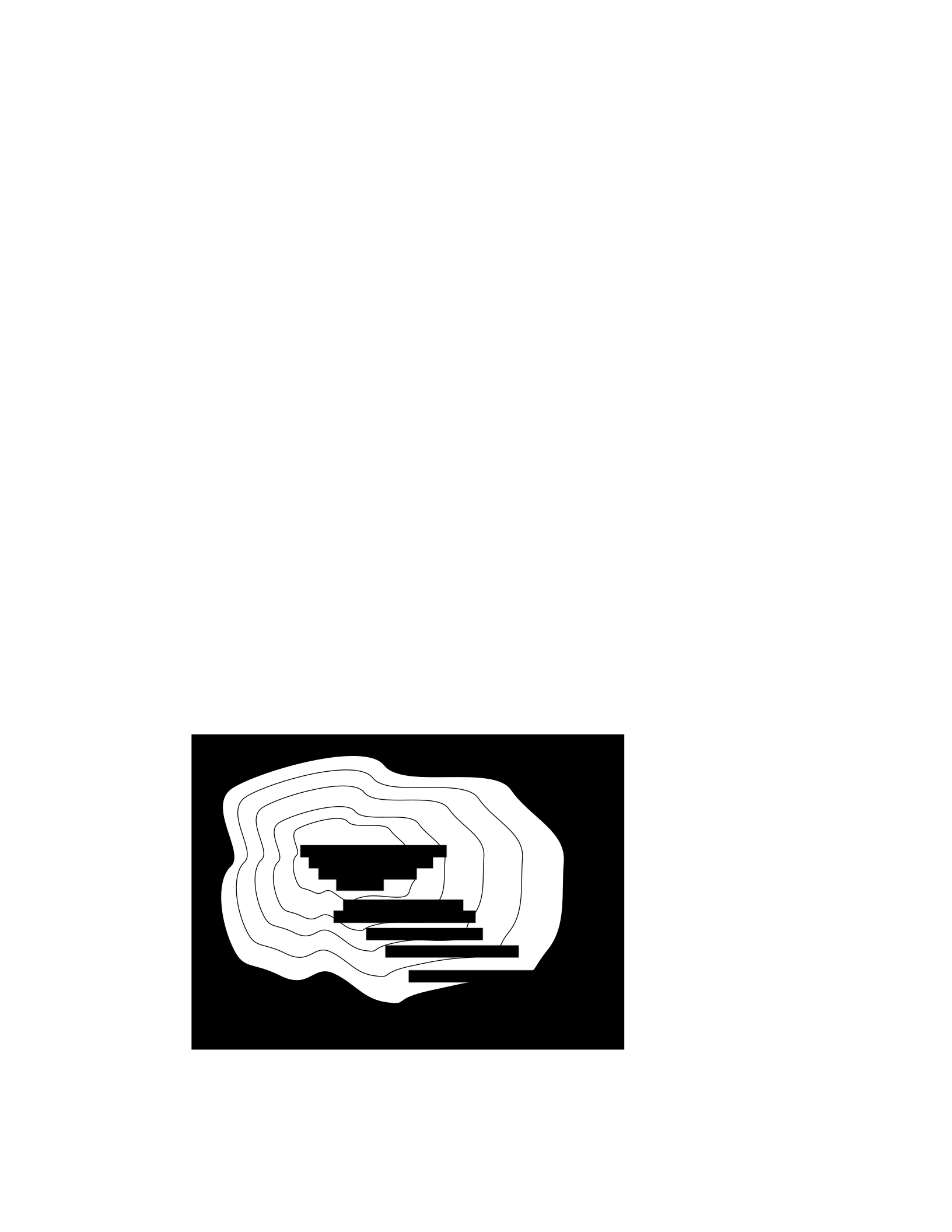
than having to re-invent the techniques yourself. And other people will be able to readily understand and
modify your designs.
We can often make a design job easier by limiting the space of possible designs, and by standardizing on:
• a basis set of primitive components;
• ways of combining the primitive components to make more complex systems;
• ways of “packaging” or abstracting pieces of a design so they can be reused (in essence creating
new “primitives”); and
• ways of capturing common patterns of abstraction (essentially, abstracting our abstractions).
Very complicated design problems can become tractable using such a primitive-combinationabstraction-
pattern (PCAP) approach. In this class, we will examine and learn to use a variety of PCAP strategies
common in EE and CS, and will even design some of our own, for special purposes. In the rest of this
section, we will hint at some of the PCAP systems we will be developing in much greater depth throughout
the class. Figure 1.1 shows one view of this development, as a successive set of restrictions of the design
space of mechanisms.
One very important thing about abstract models is that once we have fixed the abstraction, it will usually
be possible to implement it using a variety of different underlying substrates. So, as shown in figure 1.2,
we can construct general-purpose computers out of a variety of different kinds of systems, including digital
circuits and general-purpose computers. And systems satisfying the digital circuit abstraction can be
constructed from analog circuits, but also from gears or water or light.
Another demonstration of the value of abstracted models is that we can use them, by analogy, to describe
quite different systems. So, for example, the constraint models of circuits that we will study can be applied
to describing transmission of neural signals down the spinal cord, or of heat through a network of
connected bodies.
Let’s explore the abstraction hierarchy figure 1.1 in some more detail, moving up abstraction levels while
observing common patterns.
Figure 1.1 Increasingly constrained systems.
electrical systems
traditional analog circuits
digital electronic circuits
electronic computers
electronic computers
running Python programs
electronic computers with
Python programs that
select outputs by
planning

Figure 1.2 A single abstraction may have a variety of different underlying implementations.
Circuits
Typical electronics circuits are built out of a basis set of primitive components such as voltage sources,
resistors, capacitors, inductors and transistors. This set of component types was chosen to be closely
related to primitive concepts in our physical understanding of electronic systems in terms of voltage,
current, resistance, and the rate of change of those quantities over time. So, when we buy a physical
resistor, we tend to think only of its resistance; and when we buy a capacitor, we think of its ability to store
charge. But, of course, that physical resistor has some capacitance, and the capacitor, some resistance.
Still, it helps us in our designs to have devices that are as close to the ideal models as possible; and it helps
that people have been designing with these components for years, so that we can adopt the strategies
that generations of clever people have developed.
The method of combining circuit elements is to connect their terminals with conductors (wires, crimps,
solder, etc.), a process that is generically referred to as wiring. And our method of abstraction is to describe
the constraints that a circuit element exerts on the currents and voltages of terminals to which the
element is connected.
So, armed with the standard basis set of analog circuit components, we can try to build a circuit to control
our robot. We have a resistance that varies with the light level, but we need a voltage that does so, as well.
We can achieve this by using a voltage divider, which is shown in figure 1.3A. Using an abstract, constraint-
based model of the behavior of circuit components that we will
General-purpose computer
Digital circuits
T
uring
machine
Cellular
automata
Analog
electronics
Gears
Light
W
ater

study in detail later in the course, we can determine the following relationship between Vout and
Vin:
RB
Vout = Vin .
RA + RB
So, for example, if RA = RB, then Vout = Vin/2. Or, in our case, if RA actually varies with the amount
of light shining on it, then Vout will also vary with the light.
17
Vin Vin Vin
RARARA
Vout
RBRBmotor RBmotor
Figure 1.3 Voltage dividers: A. Resistor divider. B. Connected to a motor, in a way that breaks
the abstraction from part A. C. Connected to a motor, with a buffer.
That is great. So, now, we might imagine that we could use this voltage difference that we have
created to drive the motor at different speeds, depending on the light hitting the resistor, using
a circuit something like the one shown in figure 1.3B. But, sadly, that will not work. It turns out
that once we connect the motor to the circuit, it actually changes the voltages, and we can no
longer maintain the voltage difference needed to drive the motor.
So, although we have developed an abstract model of the behavior of circuit components, which
lets us analyze the behavior of a particular complete circuit design, it does not give us
modularity. That is, we cannot design two parts of a circuit, understand each of their behaviors,
and then predict the behavior of the composite system based on the behavior of the separate
components. Instead, we would have to re-analyze the joint behavior of the whole composite
system. Lack of modularity makes it very difficult to design large systems, because two different
people, or the same person at two different times, cannot design pieces and put them together
without understanding the whole.
To solve this problem, we can augment our analog-circuit toolbox with some additional
components that allow us to design components with modular behavior; they “buffer” or
“isolate” one part of the circuit from another in ways that allow us to combine the parts more
17
Do not worry if this example does not make much sense to you; we will explore this all in great detail later.

easily. In this class, we will use op-amps to build buffers, which will let us solve our sample
problem using a slightly more complex circuit, as shown in figure 1.3C.
Thus, the key point is that good modules preserve abstraction barriers between the use of a
module and internal details of how they are constructed. We will see this theme recur as we
discuss different PCAP systems.
Digital circuits
In analog circuits, we think about voltages on terminals ranging over real values. This gives us
the freedom to create an enormous variety of circuits, but sometimes that freedom actually
makes the design process more difficult. To design ever more complex circuits, we can move to
a much stronger, digital abstraction, in which the voltages on the terminals are thought of as
only taking on values that are either “low” or “high” (often called 0 and 1). This PCAP system is
made up of a basis set of elements, called gates, that are built out of simpler analog circuit
components, such as transistors and resistors. Adopting the digital abstraction is a huge
limitation on the kinds of circuits that can be built. However, digital circuits can be easy to design
and build and also can be inexpensive because the basic elements (gates) are simple (fewer
transisters are need to construct a gate than to construct an op amp), versatile (only a small
number of different kinds of logic elements are necessary to construct an arbitrary digital
circuit), and combinations are easy to think about (using Boolean logic). These properties allow
designers to build incredibly complex machines by designing small parts and putting them
together into increasingly larger pieces. Digital watches, calculators, and computers are all built
this way.
Digital design is a very important part of EECS, and it is treated in a number of our courses at
basic and advanced levels, but is not one of the topics we will go into in detail in 6.01.
Nevertheless, the same central points that we explore in this course apply to this domain as
well.
Computers
One of the most important developments in the design of digital circuits is that of the
generalpurpose “stored program” computer. Computers are a particular class of digital circuits
that are general purpose: the same actual circuit can perform (almost) any transformation
between its inputs and its outputs. Which particular transformation it performs is governed by
a program, which is some settings of physical switches, or information written on an external
physical memory, such as cards or a tape, or information stored in some sort of internal memory.
The “almost” in the previous section refers to the actual memory capacity of the computer.
Exactly what computations a computer can perform depends on the amount of memory it has;
and also on the time you are willing to wait. So, although a general-purpose computer can do
anything a special-purpose digital circuit can do, in the information-processing sense, the
computer might be slower or use more power. However, using general-purpose computers can
save an enormous amount of engineering time and effort. It is much cheaper and easier to
debug and modify and manufacture software than hardware. The modularities and abstractions
that software PCAP systems give us are even more powerful than those derived from the digital
circuit abstraction.

Again, we can see how abstraction separates use from details; we don’t need to know how the
circuits inside a computer are designed, we just need to know the rules by which we can use
them and the constraints under which they perform.
Python programs
Every general-purpose computer has a different detailed design, which means that the way its
program needs to be specified is different. Furthermore, the “machine languages” for
describing computer programs, at the most primitive level, are awkward for human
programmers. So, we have developed a number of computer programming languages for
specifying a desired computation. These languages are converted into instructions in the
computer’s native machine language by other computer programs, called compilers or
interpreters. One of the coolest and most powerful things about general-purpose computers is
this ability to write computer programs that process or create or modify other computer
programs.
Computer programming languages are PCAP systems. They provide primitive operations, ways
of combining them, ways of abstracting over them, and ways of capturing common abstraction
patterns. We will spend a considerable amount of time in this course studying the particular
primitives, combination mechanisms, and abstraction mechanisms made available in the
Python programming language. But the choice of Python is relatively unimportant. Virtually all
modern programming languages supply a similar set of mechanisms, and the choice of
programming language is primarily a matter of taste and convenience.
In a computer program we have both data primitives and computation primitives. At the most
basic level, computers generally store binary digits (bits) in groups of 32 or 64, called words.
These words are data primitives, and they can be interpreted by our programs as representing
integers, floating-point numbers, strings, or addresses of other data in the computer’s memory.
The computational primitives supported by most computers include numerical operations such
as addition and multiplication, and locating and extracting the contents of a memory at a given
address. In Python, we will work at a level of abstraction that does not require us to think very
much about addresses of data, but it is useful to understand that level of description, as well.
Primitive data and computation elements can be combined and abstracted in a variety of
different ways, depending on choices of programming style. We will explore these in more detail
in section 1.3.2.
1.2.3 Models
So far, we have discussed a number of ways of framing the problem of designing and
constructing mechanisms. Each PCAP system is accompanied by a modeling system that lets us
make mathematical models of the systems we construct.
What is a model? It is a new system that is considerably simpler than the system being modeled,
but which captures the important aspects of the original system. We might make a physical
model of an airplane to test in a wind tunnel. It does not have to have passenger seats or landing
lights; but it has to have surfaces of the correct shape, in order to capture the important
properties for this purpose. Mathematical models can capture properties of systems that are

important to us, and allow us to discover things about the system much more conveniently than
by manipulating the original system itself.
One of the hardest things about building models is deciding which aspects of the original system
to model and which ones to ignore. Many classic, dramatic engineering failures can be ascribed
to failing to model important aspects of the system. One example (which turned out to be an
ethical success story, rather than a failure) is LeMessurier’s Citicorp Building
18
, in which an
engineering design change was made, but tested in a model in which the wind came only from
a limited set of directions.
Another important dimension in modeling is whether the model is deterministic or not. We
might, for example, model the effect of the robot executing a command to set its velocity as
making an instantaneous change to the commanded velocity. But, of course, there is likely to
be some delay and some error. We have to decide whether to ignore that delay and error in our
model and treat it as if it were ideal; or, for example, to make a probabilistic model of the
possible results of that command. Generally speaking, the more different the possible outcomes
of a particular action or command, and the more diffuse the probability distribution over those
outcomes, the more important it is to explicitly include uncertainty in the model.
Once we have a model, we can use it in a variety of different ways, which we explore below.
Analytical models
By far the most prevalent use of models is in analysis: Given a circuit design, what will the
voltage on this terminal be? Given a computer program, will it compute the desired answer?
How long will it take? Given a control system, implemented as a circuit or as a program, will the
system stop at the right distance from the light bulb?
Analytical tools are important. It can be hard to verify the correctness of a system by trying it in
all possible initial conditions with all possible inputs; sometimes it is easier to develop a
mathematical model and then prove a theorem about the model.
For some systems, such as pure software computations, or the addition circuitry in a calculator,
it is possible to analyze correctness or speed with just a model of the system in question. For
other systems, such as fuel injectors, it is impossible to analyze the correctness of the controller
without also modeling the environment (or “plant”) to which it is connected, and then analyzing
the behavior of the coupled system of the controller and environment.
To demonstrate some of these tradeoffs, we can do a very simple analysis of a robot moving
toward a lamp. Imagine that we arrange it so that the robot’s velocity at time t, V[t], is
proportional to the difference between the actual light level, X[t], and a desired light level (that
is, the light level we expect to encounter when the robot is the desired distance from the lamp),
Xdesired ; that is, we can model our control system with the difference equation
18
See “The Fifty-Nine Story Crisis”, The New Yorker, May 29, 1995, pp 45-53.

V[t] = k(Xdesired − X[t]) where k is the constant of
proportionality, or gain, of the controller.
Now, we need to model the world. For simplicity, we equate the light level to the robot’s position
(assuming that the units match); in addition we assume the robot’s position at time t is its
position at time t−1 plus its velocity at time t−1 (actually, this should be the product of the
velocity and the length of time between samples, but we can just assume a unit time step and
thus use velocity). When we couple these models, we get the difference equation
X[t] = X[t − 1] + k(Xdesired − X[t − 1]) .
Now, for a given value of k, we can determine how the system will behave over time, by solving
the difference equation in X.
Later in the course, we will see how easily-determined mathematical properties of a
differenceequation model can tell us whether a control system will have the desired behavior
and whether or not the controller will cause the system to oscillate. These same kinds of
analyses can be applied to robot control systems as well as to the temporal properties of
voltages in a circuit, and even to problems as unrelated as the consequences of a monetary
policy decision in economics. It is important to note that treating the system as moving in
discrete time steps is an approximation to underlying continuous dynamics; it can make models
that are easier to analyze, but it requires sophisticated understanding of sampling to understand
the effects of this approximation on the correctness of the results.
Synthetic models
One goal of many people in a variety of sub-disciplines of computer science and electrical
engineering is automatic synthesis of systems from formal descriptions of their desired
behavior. For example, you might describe some properties you would want the input/output
behavior of a circuit or computer program to have, and then have a computer system discover
a circuit or program with the desired property.
This is a well-specified problem, but generally the search space of possible circuits or programs
is much too large for an automated process; the intuition and previous experience of an expert
human designer cannot yet be matched by computational search methods.
However, humans use informal models of systems for synthesis. The documentation of a
software library, which describes the function of the various procedures, serves as an informal
model that a programmer can use to assemble those components to build new, complex
systems.
Internal models
As we wish to build more and more complex systems with software programs as controllers, we
find that it is often useful to build additional layers of abstraction on top of the one provided by
a generic programming language. This is particularly true when the nature of the exact

computation required depends considerably on information that is only received during the
execution of the system.
Consider, for example, an automated taxi robot (or, more prosaically, the navigation system in
your new car). It takes, as input, a current location in the city and a goal location, and gives, as
output, a path from the current location to the goal. It has a map built into it.
It is theoretically possible to build an enormous digital circuit or computer program that
contains a look-up table, in which we precompute the path for all pairs of locations and store
them away. Then when we want to find a path, we could simply look in the table at the location
corresponding to the start and goal location and retrieve the precomputed path. Unfortunately,
the size of that table is too huge to contemplate. Instead, what we do is construct an abstraction
of the problem as one of finding a path from any start state to any goal state, through a graph
(an abstract mathematical construct of “nodes” with “arcs” connecting them). We can develop
and implement a general-purpose algorithm that will solve any shortest-path problem in a
graph. That algorithm and implementation will be useful for a wide variety of possible problems.
And for the navigation system, all we have to do is represent the map as a graph, specify the
start and goal states, and call the general graph-search algorithm.
We can think of this process as actually putting a model of the system’s interactions with the
world inside the controller; it can consider different courses of action in the world and pick the
one that is the best according to some criterion.
Another example of using internal models is when the system has some significant lack of
information about the state of the environment. In such situations, it may be appropriate to
explicitly model the set of possible states of the external world and their associated
probabilities, and to update this model over time as new evidence is gathered. We will pursue
an example of this approach near the end of the course.
1.3 Programming embedded systems
There are many different ways of thinking about modularity and abstraction for software.
Different models will make some things easier to say and do and others more difficult, making
different models appropriate for different tasks. In the following sections, we explore different
strategies for building software systems that interact with an external environment, and then
different strategies for specifying the purely computational part of a system.
1.3.1 Interacting with the environment
Increasingly, computer systems need to interact with the world around them, receiving
information about the external world, and taking actions to affect the world. Furthermore, the
world is dynamic, so that as the system is computing, the world is changing, requiring future
computation to adapt to the new state of the world.
There are a variety of different ways to organize computations that interact with an external
world. Generally speaking, such a computation needs to:
25. get information from sensors (light sensors, sonars, mouse, keyboard, etc.),
26. perform computation, remembering some of the results, and

27. take actions to change the outside world (move the robot, print, draw, etc.).
These operations can be put together in different styles.
1.3.1.1 Sequential
The most immediately straightforward style for constructing a program that interacts with the
world is the basic imperative style, in which the program gives a sequence of ’commands’ to the
system it is controlling. A library of special procedures is defined, some of which read
information from the sensors and others of which cause actions to be performed. Example
procedures might move a robot forward a fixed distance, or send a file out over the network, or
move video-game characters on the screen.
In this model, we could naturally write a program that moves an idealized robot in a square, if
there is space in front of it.
if noObstacleInFront:
moveDistance(1)
turnAngle(90)
moveDistance(1)
turnAngle(90)
moveDistance(1)
turnAngle(90)
moveDistance(1)
turnAngle(90)
The major problem with this style of programming is that the programmer has to remember to
check the sensors sufficiently frequently. For instance, if the robot checks for free space in front,
and then starts moving, it might turn out that a subsequent sensor reading will show that there
is something in front of the robot, either because someone walked in front of it or because the
previous reading was erroneous. It is hard to have the discipline, as a programmer, to remember
to keep checking the sensor conditions frequently enough, and the resulting programs can be
quite difficult to read and understand.
For the robot moving toward the light, we might write a program like this:
while lightValue <
desiredValue:
moveDistance(0.1)
This would have the robot creep up, step by step, toward the light. We might want to modify it
so that the robot moved a distance that was related to the difference between the current and
desired light values. However, if it takes larger steps, then during the time that it is moving it
will not be sensitive to possible changes in the light value and cannot react immediately to
them.
1.3.1.2 Event-Driven
User-interface programs are often best organized differently, as event-driven (also called
interrupt driven) programs. In this case, the program is specified as a collection of procedures

(called ’handlers’ or ’callbacks’) that are attached to particular events that can take place. So,
for example, there might be procedures that are called when the mouse is clicked on each
button in the interface, when the user types into a text field, or when the temperature of a
reactor gets too high. An “event loop” runs continuously, checking to see whether any of the
triggering events have happened, and, if they have, calling the associated procedure.
In our simple example, we might imagine writing a program that told the robot to drive forward
by default; and then install an event handler that says that if the light level reaches the desired
value, it should stop. This program would be reactive to sudden changes in the environment.
As the number and frequency of the conditions that need responses increases, it can be difficult
to both keep a program like this running well and guarantee a minimum response time to any
event.
1.3.1.3 Transducer
An alternative view is that programming a system that interacts with an external world is like
building a transducer with internal state. Think of a transducer as a processing box that runs
continuously. At regular intervals (perhaps many times per second), the transducer reads all of
the sensors, does a small amount of computation, stores some values it will need for the next
computation, and then generates output values for the actions.
This computation happens over and over and over again. Complex behavior can arise out of the
temporal pattern of inputs and outputs. So, for example, a robot might try to move forward
without hitting something by defining a procedure:
def step(): distToFront = min(frontSonarReadings)
motorOutput(gain * (distToFront - desiredDistance), 0.0)
Executed repeatedly, this program will automatically modulate the robot’s speed to be
proportional to the free space in front of it.
The main problem with the transducer approach is that it can be difficult to do tasks that are
fundamentally sequential (like the example of driving in a square, shown above). We will start
with the transducer model, and then, as described in section 4.3, we will build a new abstraction
layer on top of it that will make it easy to do sequential commands, as well.
1.3.2 Programming models
Just as there are different strategies for organizing entire software systems, there are different
strategies for formally expressing computational processes within those structures.
1.3.2.1 Imperative computation
Most of you have probably been exposed to an imperative model of computer programming, in
which we think of programs as giving a sequential set of instructions to the computer to do
something. And, in fact, that is how the internals of the processors of computers are typically
structured. So, in Java or C or C++, you write typically procedures that consist of lists of
instructions to the computer:

33. Put this value in this variable
34. Square the variable
35. Divide it by pi
36. If the result is greater than 1, return the result
In this model of computation, the primitive computational elements are basic arithmetic
operations and assignment statements. We can combine the elements using sequences of
statements, and control structures such as if, for, and while. We can abstract away from the
details of a computation by defining a procedure that does it. Now, the engineer only needs to
know the specifications of the procedure, but not the implementation details, in order to use
it.
1.3.2.2 Functional computation
Another style of programming is the functional style. In this model, we gain power through
function calls. Rather than telling the computer to do things, we ask it questions: What is 4 + 5?
What is the square root of 6? What is the largest element of the list?
These questions can all be expressed as asking for the value of a function applied to some
arguments. But where do the functions come from? The answer is, from other functions. We
start with some set of basic functions (like “plus”), and use them to construct more complex
functions.
This method would not be powerful without the mechanisms of conditional evaluation and
recursion. Conditional functions ask one question under some conditions and another question
under other conditions. Recursion is a mechanism that lets the definition of a function refer to
the function being defined. Recursion is as powerful as iteration.
In this model of computation, the primitive computational elements are typically basic
arithmetic and list operations. We combine elements using function composition (using the
output of one function as the input to another), if, and recursion. We use function definition as
a method of abstraction, and the idea of higher-order functions (passing functions as arguments
to other functions) as a way of capturing common high-level patterns.
1.3.2.3 Data structures
In either style of asking the computer to do work for us, we have another kind of modularity
and abstraction, which is centered around the organization of data.
At the most primitive level, computers operate on collections of (usually 32 or 64) bits. We can
interpret such a collection of bits as representing different things: a positive integer, a signed
integer, a floating-point number, a Boolean value (true or false), one or more characters, or an
address of some other data in the memory of the computer. Python gives us the ability to work
directly with all of these primitives, except for addresses.
There is only so much you can do with a single number, though. We would like to build computer
programs that operate on representations of documents or maps or circuits or social networks.

To do so, we need to aggregate primitive data elements into more complex data structures.
These can include lists, arrays, dictionaries, and other structures of our own devising.
Here, again, we gain the power of abstraction. We can write programs that do operations on a
data structure representing a social network, for example, without having to worry about the
details of how the social network is represented in terms of bits in the machine.
1.3.2.4 Object-oriented programming: computation + data structures
Object-oriented programming is a style that applies the ideas of modularity and abstraction to
execution and data at the same time.
An object is a data structure, together with a set of procedures that operate on the data. Basic
procedures can be written in an imperative or a functional style, but ultimately there is
imperative assignment to state variables in the object.
One major new type of abstraction in OO programming is “generic” programming. It might be
that all objects have a procedure called print associated with them. So, we can ask any object
to print itself, without having to know how it is implemented. Or, in a graphics system, we might
have a variety of different objects that know their x,y positions on the screen. So each of them
can be asked, in the same way, to say what their position is, even though they might be
represented very differently inside the objects.
In addition, most object-oriented systems support inheritance, which is a way to make new
kinds of objects by saying that they are mostly like another kind of object, but with some
exceptions.
This is another way to take advantage of abstraction.
Programming languages
Python as well as other modern programming languages, such as Java, Ruby and C++, support
all of these programming models. The programmer needs to choose which programming model
best suits the task. This is an issue that we will return to throughout the course.
1.4 Summary
We hope that this course will give you a rich set of conceptual tools and practical techniques,
as well as an appreciation of how math, modeling, and implementation can work together to
enable the design and analysis of complex computational systems that interact with the world.
Acknowledgments
Thanks to Jacob White, Hal Abelson, Tomas Lozano-Perez, Sarah Finney, Sari Canelake, Eric
Grimson, Ike Chuang, and Berthold Horn for useful comments and criticisms, and to Denny
Freeman for significant parts and most of the figures in the linear systems chapter. - LPK
1.1 Goals for 6.01
We have many goals for this course. Our primary goal is for you to learn to appreciate and use the
fundamental design principles of modularity and abstraction in a variety of contexts from electrical

engineering and computer science. To achieve this goal, we will study electrical engineering (EE) and
computer science (CS) largely from the perspective of how to build systems that interact with, and attempt
to control, an external environment. Such systems include everything from low-level controllers like heat
regulators or cardiac pacemakers, to medium-level systems like automated navigation or virtual surgery,
to high-level systems that provide more natural human-computer interfaces.
Our second goal is to show you that making mathematical models of real systems can help in the design
and analysis of those systems; and to give you practice with the difficult step of deciding which aspects of
the real world are important to the problem being solved and how to model them in ways that give insight
into the problem.
We also hope to engage you more actively in the educational process. Most of the work of this course will
not be like typical problems from the end of a chapter. You will work individually and in pairs to solve
problems that are deeper and more open-ended. There will not be a unique right answer. Argument,
explanation, and justification of approach will be more important than the answer. We hope to expose
you to the ubiquity of trade-offs in engineering design: it is rare that an approach will be best in every
dimension; some will excel in one way, others in a different way. Deciding how to make such trade-offs is
a crucial part of engineering.
Another way in which we hope to engage you in the material is by having many of you return to the course
as lab assistants in future semesters. Having a large number of lab assistants in the class means that
students can be given more open-ended problems, and have people around to help them when they are
stuck. Even more importantly, the lab assistants are meant to question the students as they go; to
challenge their understanding and help them see and evaluate a variety of approaches. This process is of
great intellectual value to student and lab assistant alike.
Finally, of course, we have the more typical goals of teaching exciting and important basic material from
electrical engineering and computer science, including modern software engineering, linear systems
analysis, electronic circuits, and decision-making. This material all has an internal elegance and beauty, as
well as crucial role in building modern EE and CS systems.
1.2 Modularity, abstraction, and modeling
Whether proving a theorem by building up from lemmas to basic theorems to more specialized results, or
designing a circuit by building up from components to modules to complex processors, or designing a
software system by building up from generic procedures to classes to class libraries, humans deal with
complexity by exploiting the power of abstraction and modularity. Without such tools, a single person
would be overwhelmed by the complexity of a system, as there is only so much detail that a single person
can consciously manage at a time.
Modularity is the idea of building components that can be re-used; and abstraction is the idea that after
constructing a module (be it software or circuits or gears), most of the details of the module construction
can be ignored and a simpler description used for module interaction (the module computes the square
root, or doubles the voltage, or changes the direction of motion).
Given basic modules, one can move up a level of abstraction and construct a new module by putting
together several previously-built modules, thinking only of their abstract descriptions, and not their
implementations. And, of course, this process can be repeated over many stages. This process gives one

the ability to construct systems with complexity far beyond what would be possible if it were necessary to
understand each component in detail.
Any module can be described in a large number of ways. We might describe the circuitry in a digital watch
in terms of how it behaves as a clock and a stopwatch, or in terms of voltages and currents within the
circuit, or in terms of the heat produced at different parts of the circuitry. Each of these is a different model
of the watch. Different models will be appropriate for different tasks: there is no single correct model.
Rather, each model exposes different dimensions of the system, allowing us to explore many aspects of
the design space of a system, and to trade off different factors in the performance of a system.
The primary theme of this course will be to learn about different methods for building modules out of
primitives, and of building different abstract models of them, so that we can analyze or predict their
behavior, and so we can recombine them into even more complex systems. The same fundamental
principles will apply to software, to control systems, and to circuits.
1.2.1 Example problem
Imagine that you need to make a robot that will roll up close to a light bulb and stop a fixed distance from
it. The first question is, how can we get electrical signals to relate to the physical phenomena of light
readings and robot wheel rotations? There is a large part of electrical engineering related to the design of
physical devices that connect to the physical world in such a way that some electrical property of the
device relates to a physical process in the world. For example, a light-sensitive resistor (photo-resistor) is
a sensor whose resistance changes depending on light intensity impinging on it; a motor is an effector
whose rotor speed is related to the voltage across its two terminals. In this course, we will not examine
the detailed physics of sensors and effectors, but will concentrate on ways of designing systems that use
sensors and effectors to perform both simple and more complicated tasks. To get a robot to stop in front
of a light bulb, the problem will be to find a way to connect the photo-resistor to the motor, so that the
robot will stop at an appropriate distance from the bulb. Thus, we will already use the idea of abstraction
to treat sensors Chapter 1 Course Overview
and effectors as primitive modules whose internal details we can ignore, and whose performance
characteristics we can use as we design systems built on these elements.
1.2.2 An abstraction hierarchy of mechanisms
Given the light-sensitive resistor and the motor, we could find many ways of connecting them, using bits
of metal and ceramic of different kinds, or making some kind of magnetic or mechanical linkages. The
space of possible designs of machines is enormous.
One of the most important things that engineers do, when faced with a set of design problems, is to
standardize on a basis set of components to use to build their systems. There are many reasons for
standardizing on a basis set of components, mostly having to do with efficiency of understanding and of
manufacturing. It is important, as a designer, to develop a repertoire of standard bits and pieces of designs
that you understand well and can put together in various ways to make more complex systems. If you use
the same basis set of components as other designers, you can learn valuable techniques from them, rather

than having to re-invent the techniques yourself. And other people will be able to readily understand and
modify your designs.
We can often make a design job easier by limiting the space of possible designs, and by standardizing on:
• a basis set of primitive components;
• ways of combining the primitive components to make more complex systems;
• ways of “packaging” or abstracting pieces of a design so they can be reused (in essence creating
new “primitives”); and
• ways of capturing common patterns of abstraction (essentially, abstracting our abstractions).
Very complicated design problems can become tractable using such a primitive-combinationabstraction-
pattern (PCAP) approach. In this class, we will examine and learn to use a variety of PCAP strategies
common in EE and CS, and will even design some of our own, for special purposes. In the rest of this
section, we will hint at some of the PCAP systems we will be developing in much greater depth throughout
the class. Figure 1.1 shows one view of this development, as a successive set of restrictions of the design
space of mechanisms.
One very important thing about abstract models is that once we have fixed the abstraction, it will usually
be possible to implement it using a variety of different underlying substrates. So, as shown in figure 1.2,
we can construct general-purpose computers out of a variety of different kinds of systems, including digital
circuits and general-purpose computers. And systems satisfying the digital circuit abstraction can be
constructed from analog circuits, but also from gears or water or light.
Another demonstration of the value of abstracted models is that we can use them, by analogy, to describe
quite different systems. So, for example, the constraint models of circuits that we will study can be applied
to describing transmission of neural signals down the spinal cord, or of heat through a network of
connected bodies.
Let’s explore the abstraction hierarchy figure 1.1 in some more detail, moving up abstraction levels while
observing common patterns.
Figure 1.1 Increasingly constrained systems.
electrical systems
traditional analog circuits
digital electronic circuits
electronic computers
electronic computers
running Python programs
electronic computers with
Python programs that
select outputs by
planning

Figure 1.2 A single abstraction may have a variety of different underlying implementations.
Circuits
Typical electronics circuits are built out of a basis set of primitive components such as voltage sources,
resistors, capacitors, inductors and transistors. This set of component types was chosen to be closely
related to primitive concepts in our physical understanding of electronic systems in terms of voltage,
current, resistance, and the rate of change of those quantities over time. So, when we buy a physical
resistor, we tend to think only of its resistance; and when we buy a capacitor, we think of its ability to store
charge. But, of course, that physical resistor has some capacitance, and the capacitor, some resistance.
Still, it helps us in our designs to have devices that are as close to the ideal models as possible; and it helps
that people have been designing with these components for years, so that we can adopt the strategies
that generations of clever people have developed.
The method of combining circuit elements is to connect their terminals with conductors (wires, crimps,
solder, etc.), a process that is generically referred to as wiring. And our method of abstraction is to describe
the constraints that a circuit element exerts on the currents and voltages of terminals to which the
element is connected.
So, armed with the standard basis set of analog circuit components, we can try to build a circuit to control
our robot. We have a resistance that varies with the light level, but we need a voltage that does so, as well.
We can achieve this by using a voltage divider, which is shown in figure 1.3A. Using an abstract, constraint-
based model of the behavior of circuit components that we will
General-purpose computer
Digital circuits
T
uring
machine
Cellular
automata
Analog
electronics
Gears
Light
W
ater

study in detail later in the course, we can determine the following relationship between Vout and
Vin:
RB
Vout = Vin .
RA + RB
So, for example, if RA = RB, then Vout = Vin/2. Or, in our case, if RA actually varies with the amount
of light shining on it, then Vout will also vary with the light.
19
Vin Vin Vin
RARARA
Vout
RBRBmotor RBmotor
Figure 1.3 Voltage dividers: A. Resistor divider. B. Connected to a motor, in a way that breaks
the abstraction from part A. C. Connected to a motor, with a buffer.
That is great. So, now, we might imagine that we could use this voltage difference that we have
created to drive the motor at different speeds, depending on the light hitting the resistor, using
a circuit something like the one shown in figure 1.3B. But, sadly, that will not work. It turns out
that once we connect the motor to the circuit, it actually changes the voltages, and we can no
longer maintain the voltage difference needed to drive the motor.
So, although we have developed an abstract model of the behavior of circuit components, which
lets us analyze the behavior of a particular complete circuit design, it does not give us
modularity. That is, we cannot design two parts of a circuit, understand each of their behaviors,
and then predict the behavior of the composite system based on the behavior of the separate
components. Instead, we would have to re-analyze the joint behavior of the whole composite
system. Lack of modularity makes it very difficult to design large systems, because two different
people, or the same person at two different times, cannot design pieces and put them together
without understanding the whole.
To solve this problem, we can augment our analog-circuit toolbox with some additional
components that allow us to design components with modular behavior; they “buffer” or
“isolate” one part of the circuit from another in ways that allow us to combine the parts more
19
Do not worry if this example does not make much sense to you; we will explore this all in great detail later.

easily. In this class, we will use op-amps to build buffers, which will let us solve our sample
problem using a slightly more complex circuit, as shown in figure 1.3C.
Thus, the key point is that good modules preserve abstraction barriers between the use of a
module and internal details of how they are constructed. We will see this theme recur as we
discuss different PCAP systems.
Digital circuits
In analog circuits, we think about voltages on terminals ranging over real values. This gives us
the freedom to create an enormous variety of circuits, but sometimes that freedom actually
makes the design process more difficult. To design ever more complex circuits, we can move to
a much stronger, digital abstraction, in which the voltages on the terminals are thought of as
only taking on values that are either “low” or “high” (often called 0 and 1). This PCAP system is
made up of a basis set of elements, called gates, that are built out of simpler analog circuit
components, such as transistors and resistors. Adopting the digital abstraction is a huge
limitation on the kinds of circuits that can be built. However, digital circuits can be easy to design
and build and also can be inexpensive because the basic elements (gates) are simple (fewer
transisters are need to construct a gate than to construct an op amp), versatile (only a small
number of different kinds of logic elements are necessary to construct an arbitrary digital
circuit), and combinations are easy to think about (using Boolean logic). These properties allow
designers to build incredibly complex machines by designing small parts and putting them
together into increasingly larger pieces. Digital watches, calculators, and computers are all built
this way.
Digital design is a very important part of EECS, and it is treated in a number of our courses at
basic and advanced levels, but is not one of the topics we will go into in detail in 6.01.
Nevertheless, the same central points that we explore in this course apply to this domain as
well.
Computers
One of the most important developments in the design of digital circuits is that of the
generalpurpose “stored program” computer. Computers are a particular class of digital circuits
that are general purpose: the same actual circuit can perform (almost) any transformation
between its inputs and its outputs. Which particular transformation it performs is governed by
a program, which is some settings of physical switches, or information written on an external
physical memory, such as cards or a tape, or information stored in some sort of internal memory.
The “almost” in the previous section refers to the actual memory capacity of the computer.
Exactly what computations a computer can perform depends on the amount of memory it has;
and also on the time you are willing to wait. So, although a general-purpose computer can do
anything a special-purpose digital circuit can do, in the information-processing sense, the
computer might be slower or use more power. However, using general-purpose computers can
save an enormous amount of engineering time and effort. It is much cheaper and easier to
debug and modify and manufacture software than hardware. The modularities and abstractions
that software PCAP systems give us are even more powerful than those derived from the digital
circuit abstraction.

Again, we can see how abstraction separates use from details; we don’t need to know how the
circuits inside a computer are designed, we just need to know the rules by which we can use
them and the constraints under which they perform.
Python programs
Every general-purpose computer has a different detailed design, which means that the way its
program needs to be specified is different. Furthermore, the “machine languages” for
describing computer programs, at the most primitive level, are awkward for human
programmers. So, we have developed a number of computer programming languages for
specifying a desired computation. These languages are converted into instructions in the
computer’s native machine language by other computer programs, called compilers or
interpreters. One of the coolest and most powerful things about general-purpose computers is
this ability to write computer programs that process or create or modify other computer
programs.
Computer programming languages are PCAP systems. They provide primitive operations, ways
of combining them, ways of abstracting over them, and ways of capturing common abstraction
patterns. We will spend a considerable amount of time in this course studying the particular
primitives, combination mechanisms, and abstraction mechanisms made available in the
Python programming language. But the choice of Python is relatively unimportant. Virtually all
modern programming languages supply a similar set of mechanisms, and the choice of
programming language is primarily a matter of taste and convenience.
In a computer program we have both data primitives and computation primitives. At the most
basic level, computers generally store binary digits (bits) in groups of 32 or 64, called words.
These words are data primitives, and they can be interpreted by our programs as representing
integers, floating-point numbers, strings, or addresses of other data in the computer’s memory.
The computational primitives supported by most computers include numerical operations such
as addition and multiplication, and locating and extracting the contents of a memory at a given
address. In Python, we will work at a level of abstraction that does not require us to think very
much about addresses of data, but it is useful to understand that level of description, as well.
Primitive data and computation elements can be combined and abstracted in a variety of
different ways, depending on choices of programming style. We will explore these in more detail
in section 1.3.2.
1.2.3 Models
So far, we have discussed a number of ways of framing the problem of designing and
constructing mechanisms. Each PCAP system is accompanied by a modeling system that lets us
make mathematical models of the systems we construct.
What is a model? It is a new system that is considerably simpler than the system being modeled,
but which captures the important aspects of the original system. We might make a physical
model of an airplane to test in a wind tunnel. It does not have to have passenger seats or landing
lights; but it has to have surfaces of the correct shape, in order to capture the important
properties for this purpose. Mathematical models can capture properties of systems that are

important to us, and allow us to discover things about the system much more conveniently than
by manipulating the original system itself.
One of the hardest things about building models is deciding which aspects of the original system
to model and which ones to ignore. Many classic, dramatic engineering failures can be ascribed
to failing to model important aspects of the system. One example (which turned out to be an
ethical success story, rather than a failure) is LeMessurier’s Citicorp Building
20
, in which an
engineering design change was made, but tested in a model in which the wind came only from
a limited set of directions.
Another important dimension in modeling is whether the model is deterministic or not. We
might, for example, model the effect of the robot executing a command to set its velocity as
making an instantaneous change to the commanded velocity. But, of course, there is likely to
be some delay and some error. We have to decide whether to ignore that delay and error in our
model and treat it as if it were ideal; or, for example, to make a probabilistic model of the
possible results of that command. Generally speaking, the more different the possible outcomes
of a particular action or command, and the more diffuse the probability distribution over those
outcomes, the more important it is to explicitly include uncertainty in the model.
Once we have a model, we can use it in a variety of different ways, which we explore below.
Analytical models
By far the most prevalent use of models is in analysis: Given a circuit design, what will the
voltage on this terminal be? Given a computer program, will it compute the desired answer?
How long will it take? Given a control system, implemented as a circuit or as a program, will the
system stop at the right distance from the light bulb?
Analytical tools are important. It can be hard to verify the correctness of a system by trying it in
all possible initial conditions with all possible inputs; sometimes it is easier to develop a
mathematical model and then prove a theorem about the model.
For some systems, such as pure software computations, or the addition circuitry in a calculator,
it is possible to analyze correctness or speed with just a model of the system in question. For
other systems, such as fuel injectors, it is impossible to analyze the correctness of the controller
without also modeling the environment (or “plant”) to which it is connected, and then analyzing
the behavior of the coupled system of the controller and environment.
To demonstrate some of these tradeoffs, we can do a very simple analysis of a robot moving
toward a lamp. Imagine that we arrange it so that the robot’s velocity at time t, V[t], is
proportional to the difference between the actual light level, X[t], and a desired light level (that
is, the light level we expect to encounter when the robot is the desired distance from the lamp),
Xdesired ; that is, we can model our control system with the difference equation
20
See “The Fifty-Nine Story Crisis”, The New Yorker, May 29, 1995, pp 45-53.

V[t] = k(Xdesired − X[t]) where k is the constant of
proportionality, or gain, of the controller.
Now, we need to model the world. For simplicity, we equate the light level to the robot’s position
(assuming that the units match); in addition we assume the robot’s position at time t is its
position at time t−1 plus its velocity at time t−1 (actually, this should be the product of the
velocity and the length of time between samples, but we can just assume a unit time step and
thus use velocity). When we couple these models, we get the difference equation
X[t] = X[t − 1] + k(Xdesired − X[t − 1]) .
Now, for a given value of k, we can determine how the system will behave over time, by solving
the difference equation in X.
Later in the course, we will see how easily-determined mathematical properties of a
differenceequation model can tell us whether a control system will have the desired behavior
and whether or not the controller will cause the system to oscillate. These same kinds of
analyses can be applied to robot control systems as well as to the temporal properties of
voltages in a circuit, and even to problems as unrelated as the consequences of a monetary
policy decision in economics. It is important to note that treating the system as moving in
discrete time steps is an approximation to underlying continuous dynamics; it can make models
that are easier to analyze, but it requires sophisticated understanding of sampling to understand
the effects of this approximation on the correctness of the results.
Synthetic models
One goal of many people in a variety of sub-disciplines of computer science and electrical
engineering is automatic synthesis of systems from formal descriptions of their desired
behavior. For example, you might describe some properties you would want the input/output
behavior of a circuit or computer program to have, and then have a computer system discover
a circuit or program with the desired property.
This is a well-specified problem, but generally the search space of possible circuits or programs
is much too large for an automated process; the intuition and previous experience of an expert
human designer cannot yet be matched by computational search methods.
However, humans use informal models of systems for synthesis. The documentation of a
software library, which describes the function of the various procedures, serves as an informal
model that a programmer can use to assemble those components to build new, complex
systems.
Internal models
As we wish to build more and more complex systems with software programs as controllers, we
find that it is often useful to build additional layers of abstraction on top of the one provided by
a generic programming language. This is particularly true when the nature of the exact

computation required depends considerably on information that is only received during the
execution of the system.
Consider, for example, an automated taxi robot (or, more prosaically, the navigation system in
your new car). It takes, as input, a current location in the city and a goal location, and gives, as
output, a path from the current location to the goal. It has a map built into it.
It is theoretically possible to build an enormous digital circuit or computer program that
contains a look-up table, in which we precompute the path for all pairs of locations and store
them away. Then when we want to find a path, we could simply look in the table at the location
corresponding to the start and goal location and retrieve the precomputed path. Unfortunately,
the size of that table is too huge to contemplate. Instead, what we do is construct an abstraction
of the problem as one of finding a path from any start state to any goal state, through a graph
(an abstract mathematical construct of “nodes” with “arcs” connecting them). We can develop
and implement a general-purpose algorithm that will solve any shortest-path problem in a
graph. That algorithm and implementation will be useful for a wide variety of possible problems.
And for the navigation system, all we have to do is represent the map as a graph, specify the
start and goal states, and call the general graph-search algorithm.
We can think of this process as actually putting a model of the system’s interactions with the
world inside the controller; it can consider different courses of action in the world and pick the
one that is the best according to some criterion.
Another example of using internal models is when the system has some significant lack of
information about the state of the environment. In such situations, it may be appropriate to
explicitly model the set of possible states of the external world and their associated
probabilities, and to update this model over time as new evidence is gathered. We will pursue
an example of this approach near the end of the course.
1.3 Programming embedded systems
There are many different ways of thinking about modularity and abstraction for software.
Different models will make some things easier to say and do and others more difficult, making
different models appropriate for different tasks. In the following sections, we explore different
strategies for building software systems that interact with an external environment, and then
different strategies for specifying the purely computational part of a system.
1.3.1 Interacting with the environment
Increasingly, computer systems need to interact with the world around them, receiving
information about the external world, and taking actions to affect the world. Furthermore, the
world is dynamic, so that as the system is computing, the world is changing, requiring future
computation to adapt to the new state of the world.
There are a variety of different ways to organize computations that interact with an external
world. Generally speaking, such a computation needs to:
28. get information from sensors (light sensors, sonars, mouse, keyboard, etc.),
29. perform computation, remembering some of the results, and

30. take actions to change the outside world (move the robot, print, draw, etc.).
These operations can be put together in different styles.
1.3.1.1 Sequential
The most immediately straightforward style for constructing a program that interacts with the
world is the basic imperative style, in which the program gives a sequence of ’commands’ to the
system it is controlling. A library of special procedures is defined, some of which read
information from the sensors and others of which cause actions to be performed. Example
procedures might move a robot forward a fixed distance, or send a file out over the network, or
move video-game characters on the screen.
In this model, we could naturally write a program that moves an idealized robot in a square, if
there is space in front of it.
if noObstacleInFront:
moveDistance(1)
turnAngle(90)
moveDistance(1)
turnAngle(90)
moveDistance(1)
turnAngle(90)
moveDistance(1)
turnAngle(90)
The major problem with this style of programming is that the programmer has to remember to
check the sensors sufficiently frequently. For instance, if the robot checks for free space in front,
and then starts moving, it might turn out that a subsequent sensor reading will show that there
is something in front of the robot, either because someone walked in front of it or because the
previous reading was erroneous. It is hard to have the discipline, as a programmer, to remember
to keep checking the sensor conditions frequently enough, and the resulting programs can be
quite difficult to read and understand.
For the robot moving toward the light, we might write a program like this:
while lightValue <
desiredValue:
moveDistance(0.1)
This would have the robot creep up, step by step, toward the light. We might want to modify it
so that the robot moved a distance that was related to the difference between the current and
desired light values. However, if it takes larger steps, then during the time that it is moving it
will not be sensitive to possible changes in the light value and cannot react immediately to
them.
1.3.1.2 Event-Driven
User-interface programs are often best organized differently, as event-driven (also called
interrupt driven) programs. In this case, the program is specified as a collection of procedures

(called ’handlers’ or ’callbacks’) that are attached to particular events that can take place. So,
for example, there might be procedures that are called when the mouse is clicked on each
button in the interface, when the user types into a text field, or when the temperature of a
reactor gets too high. An “event loop” runs continuously, checking to see whether any of the
triggering events have happened, and, if they have, calling the associated procedure.
In our simple example, we might imagine writing a program that told the robot to drive forward
by default; and then install an event handler that says that if the light level reaches the desired
value, it should stop. This program would be reactive to sudden changes in the environment.
As the number and frequency of the conditions that need responses increases, it can be difficult
to both keep a program like this running well and guarantee a minimum response time to any
event.
1.3.1.3 Transducer
An alternative view is that programming a system that interacts with an external world is like
building a transducer with internal state. Think of a transducer as a processing box that runs
continuously. At regular intervals (perhaps many times per second), the transducer reads all of
the sensors, does a small amount of computation, stores some values it will need for the next
computation, and then generates output values for the actions.
This computation happens over and over and over again. Complex behavior can arise out of the
temporal pattern of inputs and outputs. So, for example, a robot might try to move forward
without hitting something by defining a procedure:
def step(): distToFront = min(frontSonarReadings)
motorOutput(gain * (distToFront - desiredDistance), 0.0)
Executed repeatedly, this program will automatically modulate the robot’s speed to be
proportional to the free space in front of it.
The main problem with the transducer approach is that it can be difficult to do tasks that are
fundamentally sequential (like the example of driving in a square, shown above). We will start
with the transducer model, and then, as described in section 4.3, we will build a new abstraction
layer on top of it that will make it easy to do sequential commands, as well.
1.3.2 Programming models
Just as there are different strategies for organizing entire software systems, there are different
strategies for formally expressing computational processes within those structures.
1.3.2.1 Imperative computation
Most of you have probably been exposed to an imperative model of computer programming, in
which we think of programs as giving a sequential set of instructions to the computer to do
something. And, in fact, that is how the internals of the processors of computers are typically
structured. So, in Java or C or C++, you write typically procedures that consist of lists of
instructions to the computer:

37. Put this value in this variable
38. Square the variable
39. Divide it by pi
40. If the result is greater than 1, return the result
In this model of computation, the primitive computational elements are basic arithmetic
operations and assignment statements. We can combine the elements using sequences of
statements, and control structures such as if, for, and while. We can abstract away from the
details of a computation by defining a procedure that does it. Now, the engineer only needs to
know the specifications of the procedure, but not the implementation details, in order to use
it.
1.3.2.2 Functional computation
Another style of programming is the functional style. In this model, we gain power through
function calls. Rather than telling the computer to do things, we ask it questions: What is 4 + 5?
What is the square root of 6? What is the largest element of the list?
These questions can all be expressed as asking for the value of a function applied to some
arguments. But where do the functions come from? The answer is, from other functions. We
start with some set of basic functions (like “plus”), and use them to construct more complex
functions.
This method would not be powerful without the mechanisms of conditional evaluation and
recursion. Conditional functions ask one question under some conditions and another question
under other conditions. Recursion is a mechanism that lets the definition of a function refer to
the function being defined. Recursion is as powerful as iteration.
In this model of computation, the primitive computational elements are typically basic
arithmetic and list operations. We combine elements using function composition (using the
output of one function as the input to another), if, and recursion. We use function definition as
a method of abstraction, and the idea of higher-order functions (passing functions as arguments
to other functions) as a way of capturing common high-level patterns.
1.3.2.3 Data structures
In either style of asking the computer to do work for us, we have another kind of modularity
and abstraction, which is centered around the organization of data.
At the most primitive level, computers operate on collections of (usually 32 or 64) bits. We can
interpret such a collection of bits as representing different things: a positive integer, a signed
integer, a floating-point number, a Boolean value (true or false), one or more characters, or an
address of some other data in the memory of the computer. Python gives us the ability to work
directly with all of these primitives, except for addresses.
There is only so much you can do with a single number, though. We would like to build computer
programs that operate on representations of documents or maps or circuits or social networks.

To do so, we need to aggregate primitive data elements into more complex data structures.
These can include lists, arrays, dictionaries, and other structures of our own devising.
Here, again, we gain the power of abstraction. We can write programs that do operations on a
data structure representing a social network, for example, without having to worry about the
details of how the social network is represented in terms of bits in the machine.
1.3.2.4 Object-oriented programming: computation + data structures
Object-oriented programming is a style that applies the ideas of modularity and abstraction to
execution and data at the same time.
An object is a data structure, together with a set of procedures that operate on the data. Basic
procedures can be written in an imperative or a functional style, but ultimately there is
imperative assignment to state variables in the object.
One major new type of abstraction in OO programming is “generic” programming. It might be
that all objects have a procedure called print associated with them. So, we can ask any object
to print itself, without having to know how it is implemented. Or, in a graphics system, we might
have a variety of different objects that know their x,y positions on the screen. So each of them
can be asked, in the same way, to say what their position is, even though they might be
represented very differently inside the objects.
In addition, most object-oriented systems support inheritance, which is a way to make new
kinds of objects by saying that they are mostly like another kind of object, but with some
exceptions.
This is another way to take advantage of abstraction.
Programming languages
Python as well as other modern programming languages, such as Java, Ruby and C++, support
all of these programming models. The programmer needs to choose which programming model
best suits the task. This is an issue that we will return to throughout the course.
1.4 Summary
We hope that this course will give you a rich set of conceptual tools and practical techniques,
as well as an appreciation of how math, modeling, and implementation can work together to
enable the design and analysis of complex computational systems that interact with the world.
Acknowledgments
Thanks to Jacob White, Hal Abelson, Tomas Lozano-Perez, Sarah Finney, Sari Canelake, Eric
Grimson, Ike Chuang, and Berthold Horn for useful comments and criticisms, and to Denny
Freeman for significant parts and most of the figures in the linear systems chapter. - LPK
1.1 Goals for 6.01
We have many goals for this course. Our primary goal is for you to learn to appreciate and use the
fundamental design principles of modularity and abstraction in a variety of contexts from electrical

engineering and computer science. To achieve this goal, we will study electrical engineering (EE) and
computer science (CS) largely from the perspective of how to build systems that interact with, and attempt
to control, an external environment. Such systems include everything from low-level controllers like heat
regulators or cardiac pacemakers, to medium-level systems like automated navigation or virtual surgery,
to high-level systems that provide more natural human-computer interfaces.
Our second goal is to show you that making mathematical models of real systems can help in the design
and analysis of those systems; and to give you practice with the difficult step of deciding which aspects of
the real world are important to the problem being solved and how to model them in ways that give insight
into the problem.
We also hope to engage you more actively in the educational process. Most of the work of this course will
not be like typical problems from the end of a chapter. You will work individually and in pairs to solve
problems that are deeper and more open-ended. There will not be a unique right answer. Argument,
explanation, and justification of approach will be more important than the answer. We hope to expose
you to the ubiquity of trade-offs in engineering design: it is rare that an approach will be best in every
dimension; some will excel in one way, others in a different way. Deciding how to make such trade-offs is
a crucial part of engineering.
Another way in which we hope to engage you in the material is by having many of you return to the course
as lab assistants in future semesters. Having a large number of lab assistants in the class means that
students can be given more open-ended problems, and have people around to help them when they are
stuck. Even more importantly, the lab assistants are meant to question the students as they go; to
challenge their understanding and help them see and evaluate a variety of approaches. This process is of
great intellectual value to student and lab assistant alike.
Finally, of course, we have the more typical goals of teaching exciting and important basic material from
electrical engineering and computer science, including modern software engineering, linear systems
analysis, electronic circuits, and decision-making. This material all has an internal elegance and beauty, as
well as crucial role in building modern EE and CS systems.
1.2 Modularity, abstraction, and modeling
Whether proving a theorem by building up from lemmas to basic theorems to more specialized results, or
designing a circuit by building up from components to modules to complex processors, or designing a
software system by building up from generic procedures to classes to class libraries, humans deal with
complexity by exploiting the power of abstraction and modularity. Without such tools, a single person
would be overwhelmed by the complexity of a system, as there is only so much detail that a single person
can consciously manage at a time.
Modularity is the idea of building components that can be re-used; and abstraction is the idea that after
constructing a module (be it software or circuits or gears), most of the details of the module construction
can be ignored and a simpler description used for module interaction (the module computes the square
root, or doubles the voltage, or changes the direction of motion).
Given basic modules, one can move up a level of abstraction and construct a new module by putting
together several previously-built modules, thinking only of their abstract descriptions, and not their
implementations. And, of course, this process can be repeated over many stages. This process gives one

the ability to construct systems with complexity far beyond what would be possible if it were necessary to
understand each component in detail.
Any module can be described in a large number of ways. We might describe the circuitry in a digital watch
in terms of how it behaves as a clock and a stopwatch, or in terms of voltages and currents within the
circuit, or in terms of the heat produced at different parts of the circuitry. Each of these is a different model
of the watch. Different models will be appropriate for different tasks: there is no single correct model.
Rather, each model exposes different dimensions of the system, allowing us to explore many aspects of
the design space of a system, and to trade off different factors in the performance of a system.
The primary theme of this course will be to learn about different methods for building modules out of
primitives, and of building different abstract models of them, so that we can analyze or predict their
behavior, and so we can recombine them into even more complex systems. The same fundamental
principles will apply to software, to control systems, and to circuits.
1.2.1 Example problem
Imagine that you need to make a robot that will roll up close to a light bulb and stop a fixed distance from
it. The first question is, how can we get electrical signals to relate to the physical phenomena of light
readings and robot wheel rotations? There is a large part of electrical engineering related to the design of
physical devices that connect to the physical world in such a way that some electrical property of the
device relates to a physical process in the world. For example, a light-sensitive resistor (photo-resistor) is
a sensor whose resistance changes depending on light intensity impinging on it; a motor is an effector
whose rotor speed is related to the voltage across its two terminals. In this course, we will not examine
the detailed physics of sensors and effectors, but will concentrate on ways of designing systems that use
sensors and effectors to perform both simple and more complicated tasks. To get a robot to stop in front
of a light bulb, the problem will be to find a way to connect the photo-resistor to the motor, so that the
robot will stop at an appropriate distance from the bulb. Thus, we will already use the idea of abstraction
to treat sensors Chapter 1 Course Overview
and effectors as primitive modules whose internal details we can ignore, and whose performance
characteristics we can use as we design systems built on these elements.
1.2.2 An abstraction hierarchy of mechanisms
Given the light-sensitive resistor and the motor, we could find many ways of connecting them, using bits
of metal and ceramic of different kinds, or making some kind of magnetic or mechanical linkages. The
space of possible designs of machines is enormous.
One of the most important things that engineers do, when faced with a set of design problems, is to
standardize on a basis set of components to use to build their systems. There are many reasons for
standardizing on a basis set of components, mostly having to do with efficiency of understanding and of
manufacturing. It is important, as a designer, to develop a repertoire of standard bits and pieces of designs
that you understand well and can put together in various ways to make more complex systems. If you use
the same basis set of components as other designers, you can learn valuable techniques from them, rather
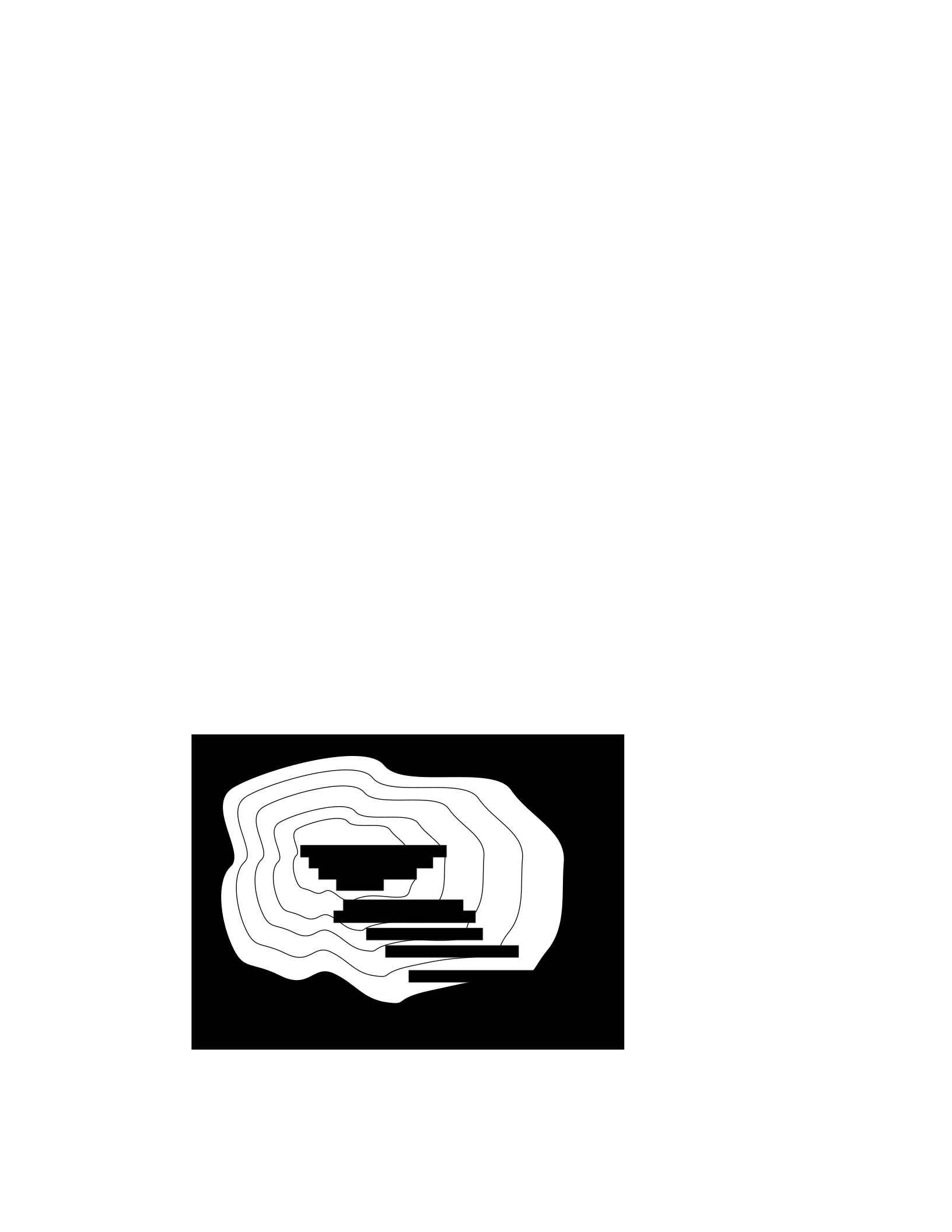
than having to re-invent the techniques yourself. And other people will be able to readily understand and
modify your designs.
We can often make a design job easier by limiting the space of possible designs, and by standardizing on:
• a basis set of primitive components;
• ways of combining the primitive components to make more complex systems;
• ways of “packaging” or abstracting pieces of a design so they can be reused (in essence creating
new “primitives”); and
• ways of capturing common patterns of abstraction (essentially, abstracting our abstractions).
Very complicated design problems can become tractable using such a primitive-combinationabstraction-
pattern (PCAP) approach. In this class, we will examine and learn to use a variety of PCAP strategies
common in EE and CS, and will even design some of our own, for special purposes. In the rest of this
section, we will hint at some of the PCAP systems we will be developing in much greater depth throughout
the class. Figure 1.1 shows one view of this development, as a successive set of restrictions of the design
space of mechanisms.
One very important thing about abstract models is that once we have fixed the abstraction, it will usually
be possible to implement it using a variety of different underlying substrates. So, as shown in figure 1.2,
we can construct general-purpose computers out of a variety of different kinds of systems, including digital
circuits and general-purpose computers. And systems satisfying the digital circuit abstraction can be
constructed from analog circuits, but also from gears or water or light.
Another demonstration of the value of abstracted models is that we can use them, by analogy, to describe
quite different systems. So, for example, the constraint models of circuits that we will study can be applied
to describing transmission of neural signals down the spinal cord, or of heat through a network of
connected bodies.
Let’s explore the abstraction hierarchy figure 1.1 in some more detail, moving up abstraction levels while
observing common patterns.
Figure 1.1 Increasingly constrained systems.
electrical systems
traditional analog circuits
digital electronic circuits
electronic computers
electronic computers
running Python programs
electronic computers with
Python programs that
select outputs by
planning

Figure 1.2 A single abstraction may have a variety of different underlying implementations.
Circuits
Typical electronics circuits are built out of a basis set of primitive components such as voltage sources,
resistors, capacitors, inductors and transistors. This set of component types was chosen to be closely
related to primitive concepts in our physical understanding of electronic systems in terms of voltage,
current, resistance, and the rate of change of those quantities over time. So, when we buy a physical
resistor, we tend to think only of its resistance; and when we buy a capacitor, we think of its ability to store
charge. But, of course, that physical resistor has some capacitance, and the capacitor, some resistance.
Still, it helps us in our designs to have devices that are as close to the ideal models as possible; and it helps
that people have been designing with these components for years, so that we can adopt the strategies
that generations of clever people have developed.
The method of combining circuit elements is to connect their terminals with conductors (wires, crimps,
solder, etc.), a process that is generically referred to as wiring. And our method of abstraction is to describe
the constraints that a circuit element exerts on the currents and voltages of terminals to which the
element is connected.
So, armed with the standard basis set of analog circuit components, we can try to build a circuit to control
our robot. We have a resistance that varies with the light level, but we need a voltage that does so, as well.
We can achieve this by using a voltage divider, which is shown in figure 1.3A. Using an abstract, constraint-
based model of the behavior of circuit components that we will
General-purpose computer
Digital circuits
T
uring
machine
Cellular
automata
Analog
electronics
Gears
Light
W
ater
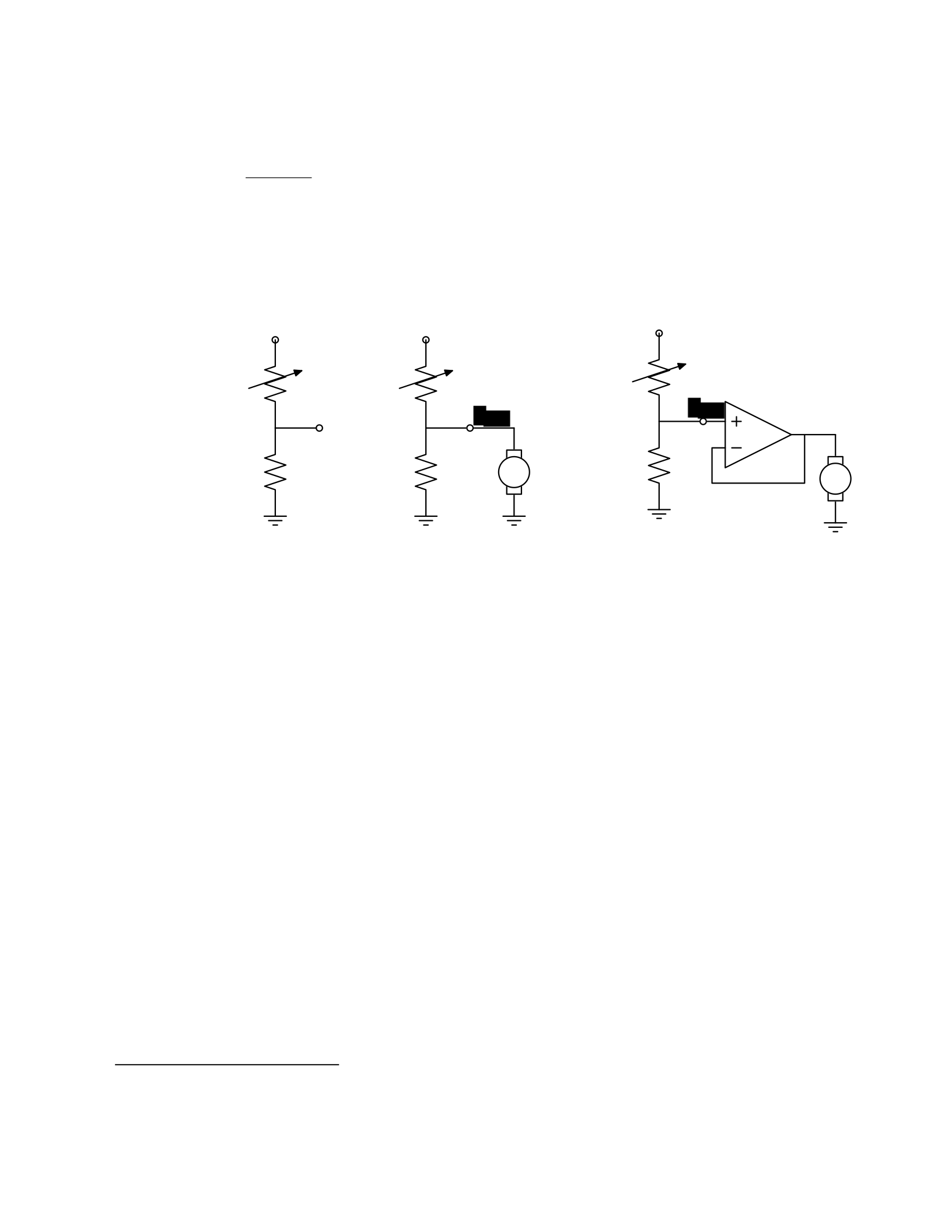
study in detail later in the course, we can determine the following relationship between Vout and
Vin:
RB
Vout = Vin .
RA + RB
So, for example, if RA = RB, then Vout = Vin/2. Or, in our case, if RA actually varies with the amount
of light shining on it, then Vout will also vary with the light.
21
Vin Vin Vin
RARARA
Vout
RBRBmotor RBmotor
Figure 1.3 Voltage dividers: A. Resistor divider. B. Connected to a motor, in a way that breaks
the abstraction from part A. C. Connected to a motor, with a buffer.
That is great. So, now, we might imagine that we could use this voltage difference that we have
created to drive the motor at different speeds, depending on the light hitting the resistor, using
a circuit something like the one shown in figure 1.3B. But, sadly, that will not work. It turns out
that once we connect the motor to the circuit, it actually changes the voltages, and we can no
longer maintain the voltage difference needed to drive the motor.
So, although we have developed an abstract model of the behavior of circuit components, which
lets us analyze the behavior of a particular complete circuit design, it does not give us
modularity. That is, we cannot design two parts of a circuit, understand each of their behaviors,
and then predict the behavior of the composite system based on the behavior of the separate
components. Instead, we would have to re-analyze the joint behavior of the whole composite
system. Lack of modularity makes it very difficult to design large systems, because two different
people, or the same person at two different times, cannot design pieces and put them together
without understanding the whole.
To solve this problem, we can augment our analog-circuit toolbox with some additional
components that allow us to design components with modular behavior; they “buffer” or
“isolate” one part of the circuit from another in ways that allow us to combine the parts more
21
Do not worry if this example does not make much sense to you; we will explore this all in great detail later.

easily. In this class, we will use op-amps to build buffers, which will let us solve our sample
problem using a slightly more complex circuit, as shown in figure 1.3C.
Thus, the key point is that good modules preserve abstraction barriers between the use of a
module and internal details of how they are constructed. We will see this theme recur as we
discuss different PCAP systems.
Digital circuits
In analog circuits, we think about voltages on terminals ranging over real values. This gives us
the freedom to create an enormous variety of circuits, but sometimes that freedom actually
makes the design process more difficult. To design ever more complex circuits, we can move to
a much stronger, digital abstraction, in which the voltages on the terminals are thought of as
only taking on values that are either “low” or “high” (often called 0 and 1). This PCAP system is
made up of a basis set of elements, called gates, that are built out of simpler analog circuit
components, such as transistors and resistors. Adopting the digital abstraction is a huge
limitation on the kinds of circuits that can be built. However, digital circuits can be easy to design
and build and also can be inexpensive because the basic elements (gates) are simple (fewer
transisters are need to construct a gate than to construct an op amp), versatile (only a small
number of different kinds of logic elements are necessary to construct an arbitrary digital
circuit), and combinations are easy to think about (using Boolean logic). These properties allow
designers to build incredibly complex machines by designing small parts and putting them
together into increasingly larger pieces. Digital watches, calculators, and computers are all built
this way.
Digital design is a very important part of EECS, and it is treated in a number of our courses at
basic and advanced levels, but is not one of the topics we will go into in detail in 6.01.
Nevertheless, the same central points that we explore in this course apply to this domain as
well.
Computers
One of the most important developments in the design of digital circuits is that of the
generalpurpose “stored program” computer. Computers are a particular class of digital circuits
that are general purpose: the same actual circuit can perform (almost) any transformation
between its inputs and its outputs. Which particular transformation it performs is governed by
a program, which is some settings of physical switches, or information written on an external
physical memory, such as cards or a tape, or information stored in some sort of internal memory.
The “almost” in the previous section refers to the actual memory capacity of the computer.
Exactly what computations a computer can perform depends on the amount of memory it has;
and also on the time you are willing to wait. So, although a general-purpose computer can do
anything a special-purpose digital circuit can do, in the information-processing sense, the
computer might be slower or use more power. However, using general-purpose computers can
save an enormous amount of engineering time and effort. It is much cheaper and easier to
debug and modify and manufacture software than hardware. The modularities and abstractions
that software PCAP systems give us are even more powerful than those derived from the digital
circuit abstraction.

Again, we can see how abstraction separates use from details; we don’t need to know how the
circuits inside a computer are designed, we just need to know the rules by which we can use
them and the constraints under which they perform.
Python programs
Every general-purpose computer has a different detailed design, which means that the way its
program needs to be specified is different. Furthermore, the “machine languages” for
describing computer programs, at the most primitive level, are awkward for human
programmers. So, we have developed a number of computer programming languages for
specifying a desired computation. These languages are converted into instructions in the
computer’s native machine language by other computer programs, called compilers or
interpreters. One of the coolest and most powerful things about general-purpose computers is
this ability to write computer programs that process or create or modify other computer
programs.
Computer programming languages are PCAP systems. They provide primitive operations, ways
of combining them, ways of abstracting over them, and ways of capturing common abstraction
patterns. We will spend a considerable amount of time in this course studying the particular
primitives, combination mechanisms, and abstraction mechanisms made available in the
Python programming language. But the choice of Python is relatively unimportant. Virtually all
modern programming languages supply a similar set of mechanisms, and the choice of
programming language is primarily a matter of taste and convenience.
In a computer program we have both data primitives and computation primitives. At the most
basic level, computers generally store binary digits (bits) in groups of 32 or 64, called words.
These words are data primitives, and they can be interpreted by our programs as representing
integers, floating-point numbers, strings, or addresses of other data in the computer’s memory.
The computational primitives supported by most computers include numerical operations such
as addition and multiplication, and locating and extracting the contents of a memory at a given
address. In Python, we will work at a level of abstraction that does not require us to think very
much about addresses of data, but it is useful to understand that level of description, as well.
Primitive data and computation elements can be combined and abstracted in a variety of
different ways, depending on choices of programming style. We will explore these in more detail
in section 1.3.2.
1.2.3 Models
So far, we have discussed a number of ways of framing the problem of designing and
constructing mechanisms. Each PCAP system is accompanied by a modeling system that lets us
make mathematical models of the systems we construct.
What is a model? It is a new system that is considerably simpler than the system being modeled,
but which captures the important aspects of the original system. We might make a physical
model of an airplane to test in a wind tunnel. It does not have to have passenger seats or landing
lights; but it has to have surfaces of the correct shape, in order to capture the important
properties for this purpose. Mathematical models can capture properties of systems that are

important to us, and allow us to discover things about the system much more conveniently than
by manipulating the original system itself.
One of the hardest things about building models is deciding which aspects of the original system
to model and which ones to ignore. Many classic, dramatic engineering failures can be ascribed
to failing to model important aspects of the system. One example (which turned out to be an
ethical success story, rather than a failure) is LeMessurier’s Citicorp Building
22
, in which an
engineering design change was made, but tested in a model in which the wind came only from
a limited set of directions.
Another important dimension in modeling is whether the model is deterministic or not. We
might, for example, model the effect of the robot executing a command to set its velocity as
making an instantaneous change to the commanded velocity. But, of course, there is likely to
be some delay and some error. We have to decide whether to ignore that delay and error in our
model and treat it as if it were ideal; or, for example, to make a probabilistic model of the
possible results of that command. Generally speaking, the more different the possible outcomes
of a particular action or command, and the more diffuse the probability distribution over those
outcomes, the more important it is to explicitly include uncertainty in the model.
Once we have a model, we can use it in a variety of different ways, which we explore below.
Analytical models
By far the most prevalent use of models is in analysis: Given a circuit design, what will the
voltage on this terminal be? Given a computer program, will it compute the desired answer?
How long will it take? Given a control system, implemented as a circuit or as a program, will the
system stop at the right distance from the light bulb?
Analytical tools are important. It can be hard to verify the correctness of a system by trying it in
all possible initial conditions with all possible inputs; sometimes it is easier to develop a
mathematical model and then prove a theorem about the model.
For some systems, such as pure software computations, or the addition circuitry in a calculator,
it is possible to analyze correctness or speed with just a model of the system in question. For
other systems, such as fuel injectors, it is impossible to analyze the correctness of the controller
without also modeling the environment (or “plant”) to which it is connected, and then analyzing
the behavior of the coupled system of the controller and environment.
To demonstrate some of these tradeoffs, we can do a very simple analysis of a robot moving
toward a lamp. Imagine that we arrange it so that the robot’s velocity at time t, V[t], is
proportional to the difference between the actual light level, X[t], and a desired light level (that
is, the light level we expect to encounter when the robot is the desired distance from the lamp),
Xdesired ; that is, we can model our control system with the difference equation
22
See “The Fifty-Nine Story Crisis”, The New Yorker, May 29, 1995, pp 45-53.

V[t] = k(Xdesired − X[t]) where k is the constant of
proportionality, or gain, of the controller.
Now, we need to model the world. For simplicity, we equate the light level to the robot’s position
(assuming that the units match); in addition we assume the robot’s position at time t is its
position at time t−1 plus its velocity at time t−1 (actually, this should be the product of the
velocity and the length of time between samples, but we can just assume a unit time step and
thus use velocity). When we couple these models, we get the difference equation
X[t] = X[t − 1] + k(Xdesired − X[t − 1]) .
Now, for a given value of k, we can determine how the system will behave over time, by solving
the difference equation in X.
Later in the course, we will see how easily-determined mathematical properties of a
differenceequation model can tell us whether a control system will have the desired behavior
and whether or not the controller will cause the system to oscillate. These same kinds of
analyses can be applied to robot control systems as well as to the temporal properties of
voltages in a circuit, and even to problems as unrelated as the consequences of a monetary
policy decision in economics. It is important to note that treating the system as moving in
discrete time steps is an approximation to underlying continuous dynamics; it can make models
that are easier to analyze, but it requires sophisticated understanding of sampling to understand
the effects of this approximation on the correctness of the results.
Synthetic models
One goal of many people in a variety of sub-disciplines of computer science and electrical
engineering is automatic synthesis of systems from formal descriptions of their desired
behavior. For example, you might describe some properties you would want the input/output
behavior of a circuit or computer program to have, and then have a computer system discover
a circuit or program with the desired property.
This is a well-specified problem, but generally the search space of possible circuits or programs
is much too large for an automated process; the intuition and previous experience of an expert
human designer cannot yet be matched by computational search methods.
However, humans use informal models of systems for synthesis. The documentation of a
software library, which describes the function of the various procedures, serves as an informal
model that a programmer can use to assemble those components to build new, complex
systems.
Internal models
As we wish to build more and more complex systems with software programs as controllers, we
find that it is often useful to build additional layers of abstraction on top of the one provided by
a generic programming language. This is particularly true when the nature of the exact

computation required depends considerably on information that is only received during the
execution of the system.
Consider, for example, an automated taxi robot (or, more prosaically, the navigation system in
your new car). It takes, as input, a current location in the city and a goal location, and gives, as
output, a path from the current location to the goal. It has a map built into it.
It is theoretically possible to build an enormous digital circuit or computer program that
contains a look-up table, in which we precompute the path for all pairs of locations and store
them away. Then when we want to find a path, we could simply look in the table at the location
corresponding to the start and goal location and retrieve the precomputed path. Unfortunately,
the size of that table is too huge to contemplate. Instead, what we do is construct an abstraction
of the problem as one of finding a path from any start state to any goal state, through a graph
(an abstract mathematical construct of “nodes” with “arcs” connecting them). We can develop
and implement a general-purpose algorithm that will solve any shortest-path problem in a
graph. That algorithm and implementation will be useful for a wide variety of possible problems.
And for the navigation system, all we have to do is represent the map as a graph, specify the
start and goal states, and call the general graph-search algorithm.
We can think of this process as actually putting a model of the system’s interactions with the
world inside the controller; it can consider different courses of action in the world and pick the
one that is the best according to some criterion.
Another example of using internal models is when the system has some significant lack of
information about the state of the environment. In such situations, it may be appropriate to
explicitly model the set of possible states of the external world and their associated
probabilities, and to update this model over time as new evidence is gathered. We will pursue
an example of this approach near the end of the course.
1.3 Programming embedded systems
There are many different ways of thinking about modularity and abstraction for software.
Different models will make some things easier to say and do and others more difficult, making
different models appropriate for different tasks. In the following sections, we explore different
strategies for building software systems that interact with an external environment, and then
different strategies for specifying the purely computational part of a system.
1.3.1 Interacting with the environment
Increasingly, computer systems need to interact with the world around them, receiving
information about the external world, and taking actions to affect the world. Furthermore, the
world is dynamic, so that as the system is computing, the world is changing, requiring future
computation to adapt to the new state of the world.
There are a variety of different ways to organize computations that interact with an external
world. Generally speaking, such a computation needs to:
31. get information from sensors (light sensors, sonars, mouse, keyboard, etc.),
32. perform computation, remembering some of the results, and

33. take actions to change the outside world (move the robot, print, draw, etc.).
These operations can be put together in different styles.
1.3.1.1 Sequential
The most immediately straightforward style for constructing a program that interacts with the
world is the basic imperative style, in which the program gives a sequence of ’commands’ to the
system it is controlling. A library of special procedures is defined, some of which read
information from the sensors and others of which cause actions to be performed. Example
procedures might move a robot forward a fixed distance, or send a file out over the network, or
move video-game characters on the screen.
In this model, we could naturally write a program that moves an idealized robot in a square, if
there is space in front of it.
if noObstacleInFront:
moveDistance(1)
turnAngle(90)
moveDistance(1)
turnAngle(90)
moveDistance(1)
turnAngle(90)
moveDistance(1)
turnAngle(90)
The major problem with this style of programming is that the programmer has to remember to
check the sensors sufficiently frequently. For instance, if the robot checks for free space in front,
and then starts moving, it might turn out that a subsequent sensor reading will show that there
is something in front of the robot, either because someone walked in front of it or because the
previous reading was erroneous. It is hard to have the discipline, as a programmer, to remember
to keep checking the sensor conditions frequently enough, and the resulting programs can be
quite difficult to read and understand.
For the robot moving toward the light, we might write a program like this:
while lightValue <
desiredValue:
moveDistance(0.1)
This would have the robot creep up, step by step, toward the light. We might want to modify it
so that the robot moved a distance that was related to the difference between the current and
desired light values. However, if it takes larger steps, then during the time that it is moving it
will not be sensitive to possible changes in the light value and cannot react immediately to
them.
1.3.1.2 Event-Driven
User-interface programs are often best organized differently, as event-driven (also called
interrupt driven) programs. In this case, the program is specified as a collection of procedures

(called ’handlers’ or ’callbacks’) that are attached to particular events that can take place. So,
for example, there might be procedures that are called when the mouse is clicked on each
button in the interface, when the user types into a text field, or when the temperature of a
reactor gets too high. An “event loop” runs continuously, checking to see whether any of the
triggering events have happened, and, if they have, calling the associated procedure.
In our simple example, we might imagine writing a program that told the robot to drive forward
by default; and then install an event handler that says that if the light level reaches the desired
value, it should stop. This program would be reactive to sudden changes in the environment.
As the number and frequency of the conditions that need responses increases, it can be difficult
to both keep a program like this running well and guarantee a minimum response time to any
event.
1.3.1.3 Transducer
An alternative view is that programming a system that interacts with an external world is like
building a transducer with internal state. Think of a transducer as a processing box that runs
continuously. At regular intervals (perhaps many times per second), the transducer reads all of
the sensors, does a small amount of computation, stores some values it will need for the next
computation, and then generates output values for the actions.
This computation happens over and over and over again. Complex behavior can arise out of the
temporal pattern of inputs and outputs. So, for example, a robot might try to move forward
without hitting something by defining a procedure:
def step(): distToFront = min(frontSonarReadings)
motorOutput(gain * (distToFront - desiredDistance), 0.0)
Executed repeatedly, this program will automatically modulate the robot’s speed to be
proportional to the free space in front of it.
The main problem with the transducer approach is that it can be difficult to do tasks that are
fundamentally sequential (like the example of driving in a square, shown above). We will start
with the transducer model, and then, as described in section 4.3, we will build a new abstraction
layer on top of it that will make it easy to do sequential commands, as well.
1.3.2 Programming models
Just as there are different strategies for organizing entire software systems, there are different
strategies for formally expressing computational processes within those structures.
1.3.2.1 Imperative computation
Most of you have probably been exposed to an imperative model of computer programming, in
which we think of programs as giving a sequential set of instructions to the computer to do
something. And, in fact, that is how the internals of the processors of computers are typically
structured. So, in Java or C or C++, you write typically procedures that consist of lists of
instructions to the computer:

41. Put this value in this variable
42. Square the variable
43. Divide it by pi
44. If the result is greater than 1, return the result
In this model of computation, the primitive computational elements are basic arithmetic
operations and assignment statements. We can combine the elements using sequences of
statements, and control structures such as if, for, and while. We can abstract away from the
details of a computation by defining a procedure that does it. Now, the engineer only needs to
know the specifications of the procedure, but not the implementation details, in order to use
it.
1.3.2.2 Functional computation
Another style of programming is the functional style. In this model, we gain power through
function calls. Rather than telling the computer to do things, we ask it questions: What is 4 + 5?
What is the square root of 6? What is the largest element of the list?
These questions can all be expressed as asking for the value of a function applied to some
arguments. But where do the functions come from? The answer is, from other functions. We
start with some set of basic functions (like “plus”), and use them to construct more complex
functions.
This method would not be powerful without the mechanisms of conditional evaluation and
recursion. Conditional functions ask one question under some conditions and another question
under other conditions. Recursion is a mechanism that lets the definition of a function refer to
the function being defined. Recursion is as powerful as iteration.
In this model of computation, the primitive computational elements are typically basic
arithmetic and list operations. We combine elements using function composition (using the
output of one function as the input to another), if, and recursion. We use function definition as
a method of abstraction, and the idea of higher-order functions (passing functions as arguments
to other functions) as a way of capturing common high-level patterns.
1.3.2.3 Data structures
In either style of asking the computer to do work for us, we have another kind of modularity
and abstraction, which is centered around the organization of data.
At the most primitive level, computers operate on collections of (usually 32 or 64) bits. We can
interpret such a collection of bits as representing different things: a positive integer, a signed
integer, a floating-point number, a Boolean value (true or false), one or more characters, or an
address of some other data in the memory of the computer. Python gives us the ability to work
directly with all of these primitives, except for addresses.
There is only so much you can do with a single number, though. We would like to build computer
programs that operate on representations of documents or maps or circuits or social networks.

To do so, we need to aggregate primitive data elements into more complex data structures.
These can include lists, arrays, dictionaries, and other structures of our own devising.
Here, again, we gain the power of abstraction. We can write programs that do operations on a
data structure representing a social network, for example, without having to worry about the
details of how the social network is represented in terms of bits in the machine.
1.3.2.4 Object-oriented programming: computation + data structures
Object-oriented programming is a style that applies the ideas of modularity and abstraction to
execution and data at the same time.
An object is a data structure, together with a set of procedures that operate on the data. Basic
procedures can be written in an imperative or a functional style, but ultimately there is
imperative assignment to state variables in the object.
One major new type of abstraction in OO programming is “generic” programming. It might be
that all objects have a procedure called print associated with them. So, we can ask any object
to print itself, without having to know how it is implemented. Or, in a graphics system, we might
have a variety of different objects that know their x,y positions on the screen. So each of them
can be asked, in the same way, to say what their position is, even though they might be
represented very differently inside the objects.
In addition, most object-oriented systems support inheritance, which is a way to make new
kinds of objects by saying that they are mostly like another kind of object, but with some
exceptions.
This is another way to take advantage of abstraction.
Programming languages
Python as well as other modern programming languages, such as Java, Ruby and C++, support
all of these programming models. The programmer needs to choose which programming model
best suits the task. This is an issue that we will return to throughout the course.
1.4 Summary
We hope that this course will give you a rich set of conceptual tools and practical techniques,
as well as an appreciation of how math, modeling, and implementation can work together to
enable the design and analysis of complex computational systems that interact with the world.
Acknowledgments
Thanks to Jacob White, Hal Abelson, Tomas Lozano-Perez, Sarah Finney, Sari Canelake, Eric
Grimson, Ike Chuang, and Berthold Horn for useful comments and criticisms, and to Denny
Freeman for significant parts and most of the figures in the linear systems chapter. - LPK
1.1 Goals for 6.01
We have many goals for this course. Our primary goal is for you to learn to appreciate and use the
fundamental design principles of modularity and abstraction in a variety of contexts from electrical

engineering and computer science. To achieve this goal, we will study electrical engineering (EE) and
computer science (CS) largely from the perspective of how to build systems that interact with, and attempt
to control, an external environment. Such systems include everything from low-level controllers like heat
regulators or cardiac pacemakers, to medium-level systems like automated navigation or virtual surgery,
to high-level systems that provide more natural human-computer interfaces.
Our second goal is to show you that making mathematical models of real systems can help in the design
and analysis of those systems; and to give you practice with the difficult step of deciding which aspects of
the real world are important to the problem being solved and how to model them in ways that give insight
into the problem.
We also hope to engage you more actively in the educational process. Most of the work of this course will
not be like typical problems from the end of a chapter. You will work individually and in pairs to solve
problems that are deeper and more open-ended. There will not be a unique right answer. Argument,
explanation, and justification of approach will be more important than the answer. We hope to expose
you to the ubiquity of trade-offs in engineering design: it is rare that an approach will be best in every
dimension; some will excel in one way, others in a different way. Deciding how to make such trade-offs is
a crucial part of engineering.
Another way in which we hope to engage you in the material is by having many of you return to the course
as lab assistants in future semesters. Having a large number of lab assistants in the class means that
students can be given more open-ended problems, and have people around to help them when they are
stuck. Even more importantly, the lab assistants are meant to question the students as they go; to
challenge their understanding and help them see and evaluate a variety of approaches. This process is of
great intellectual value to student and lab assistant alike.
Finally, of course, we have the more typical goals of teaching exciting and important basic material from
electrical engineering and computer science, including modern software engineering, linear systems
analysis, electronic circuits, and decision-making. This material all has an internal elegance and beauty, as
well as crucial role in building modern EE and CS systems.
1.2 Modularity, abstraction, and modeling
Whether proving a theorem by building up from lemmas to basic theorems to more specialized results, or
designing a circuit by building up from components to modules to complex processors, or designing a
software system by building up from generic procedures to classes to class libraries, humans deal with
complexity by exploiting the power of abstraction and modularity. Without such tools, a single person
would be overwhelmed by the complexity of a system, as there is only so much detail that a single person
can consciously manage at a time.
Modularity is the idea of building components that can be re-used; and abstraction is the idea that after
constructing a module (be it software or circuits or gears), most of the details of the module construction
can be ignored and a simpler description used for module interaction (the module computes the square
root, or doubles the voltage, or changes the direction of motion).
Given basic modules, one can move up a level of abstraction and construct a new module by putting
together several previously-built modules, thinking only of their abstract descriptions, and not their
implementations. And, of course, this process can be repeated over many stages. This process gives one

the ability to construct systems with complexity far beyond what would be possible if it were necessary to
understand each component in detail.
Any module can be described in a large number of ways. We might describe the circuitry in a digital watch
in terms of how it behaves as a clock and a stopwatch, or in terms of voltages and currents within the
circuit, or in terms of the heat produced at different parts of the circuitry. Each of these is a different model
of the watch. Different models will be appropriate for different tasks: there is no single correct model.
Rather, each model exposes different dimensions of the system, allowing us to explore many aspects of
the design space of a system, and to trade off different factors in the performance of a system.
The primary theme of this course will be to learn about different methods for building modules out of
primitives, and of building different abstract models of them, so that we can analyze or predict their
behavior, and so we can recombine them into even more complex systems. The same fundamental
principles will apply to software, to control systems, and to circuits.
1.2.1 Example problem
Imagine that you need to make a robot that will roll up close to a light bulb and stop a fixed distance from
it. The first question is, how can we get electrical signals to relate to the physical phenomena of light
readings and robot wheel rotations? There is a large part of electrical engineering related to the design of
physical devices that connect to the physical world in such a way that some electrical property of the
device relates to a physical process in the world. For example, a light-sensitive resistor (photo-resistor) is
a sensor whose resistance changes depending on light intensity impinging on it; a motor is an effector
whose rotor speed is related to the voltage across its two terminals. In this course, we will not examine
the detailed physics of sensors and effectors, but will concentrate on ways of designing systems that use
sensors and effectors to perform both simple and more complicated tasks. To get a robot to stop in front
of a light bulb, the problem will be to find a way to connect the photo-resistor to the motor, so that the
robot will stop at an appropriate distance from the bulb. Thus, we will already use the idea of abstraction
to treat sensors Chapter 1 Course Overview
and effectors as primitive modules whose internal details we can ignore, and whose performance
characteristics we can use as we design systems built on these elements.
1.2.2 An abstraction hierarchy of mechanisms
Given the light-sensitive resistor and the motor, we could find many ways of connecting them, using bits
of metal and ceramic of different kinds, or making some kind of magnetic or mechanical linkages. The
space of possible designs of machines is enormous.
One of the most important things that engineers do, when faced with a set of design problems, is to
standardize on a basis set of components to use to build their systems. There are many reasons for
standardizing on a basis set of components, mostly having to do with efficiency of understanding and of
manufacturing. It is important, as a designer, to develop a repertoire of standard bits and pieces of designs
that you understand well and can put together in various ways to make more complex systems. If you use
the same basis set of components as other designers, you can learn valuable techniques from them, rather

than having to re-invent the techniques yourself. And other people will be able to readily understand and
modify your designs.
We can often make a design job easier by limiting the space of possible designs, and by standardizing on:
• a basis set of primitive components;
• ways of combining the primitive components to make more complex systems;
• ways of “packaging” or abstracting pieces of a design so they can be reused (in essence creating
new “primitives”); and
• ways of capturing common patterns of abstraction (essentially, abstracting our abstractions).
Very complicated design problems can become tractable using such a primitive-combinationabstraction-
pattern (PCAP) approach. In this class, we will examine and learn to use a variety of PCAP strategies
common in EE and CS, and will even design some of our own, for special purposes. In the rest of this
section, we will hint at some of the PCAP systems we will be developing in much greater depth throughout
the class. Figure 1.1 shows one view of this development, as a successive set of restrictions of the design
space of mechanisms.
One very important thing about abstract models is that once we have fixed the abstraction, it will usually
be possible to implement it using a variety of different underlying substrates. So, as shown in figure 1.2,
we can construct general-purpose computers out of a variety of different kinds of systems, including digital
circuits and general-purpose computers. And systems satisfying the digital circuit abstraction can be
constructed from analog circuits, but also from gears or water or light.
Another demonstration of the value of abstracted models is that we can use them, by analogy, to describe
quite different systems. So, for example, the constraint models of circuits that we will study can be applied
to describing transmission of neural signals down the spinal cord, or of heat through a network of
connected bodies.
Let’s explore the abstraction hierarchy figure 1.1 in some more detail, moving up abstraction levels while
observing common patterns.
Figure 1.1 Increasingly constrained systems.
electrical systems
traditional analog circuits
digital electronic circuits
electronic computers
electronic computers
running Python programs
electronic computers with
Python programs that
select outputs by
planning

Figure 1.2 A single abstraction may have a variety of different underlying implementations.
Circuits
Typical electronics circuits are built out of a basis set of primitive components such as voltage sources,
resistors, capacitors, inductors and transistors. This set of component types was chosen to be closely
related to primitive concepts in our physical understanding of electronic systems in terms of voltage,
current, resistance, and the rate of change of those quantities over time. So, when we buy a physical
resistor, we tend to think only of its resistance; and when we buy a capacitor, we think of its ability to store
charge. But, of course, that physical resistor has some capacitance, and the capacitor, some resistance.
Still, it helps us in our designs to have devices that are as close to the ideal models as possible; and it helps
that people have been designing with these components for years, so that we can adopt the strategies
that generations of clever people have developed.
The method of combining circuit elements is to connect their terminals with conductors (wires, crimps,
solder, etc.), a process that is generically referred to as wiring. And our method of abstraction is to describe
the constraints that a circuit element exerts on the currents and voltages of terminals to which the
element is connected.
So, armed with the standard basis set of analog circuit components, we can try to build a circuit to control
our robot. We have a resistance that varies with the light level, but we need a voltage that does so, as well.
We can achieve this by using a voltage divider, which is shown in figure 1.3A. Using an abstract, constraint-
based model of the behavior of circuit components that we will
General-purpose computer
Digital circuits
T
uring
machine
Cellular
automata
Analog
electronics
Gears
Light
W
ater
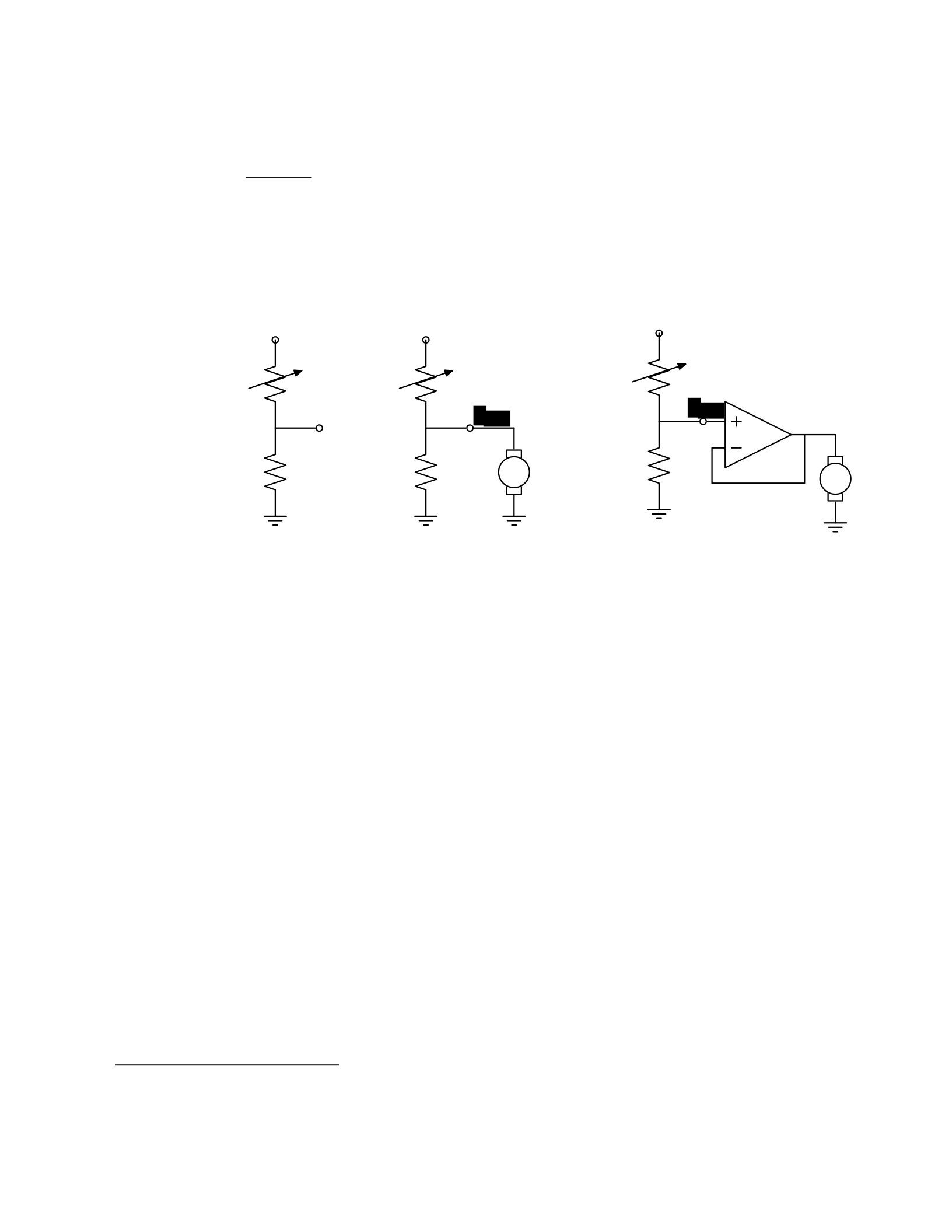
study in detail later in the course, we can determine the following relationship between Vout and
Vin:
RB
Vout = Vin .
RA + RB
So, for example, if RA = RB, then Vout = Vin/2. Or, in our case, if RA actually varies with the amount
of light shining on it, then Vout will also vary with the light.
23
Vin Vin Vin
RARARA
Vout
RBRBmotor RBmotor
Figure 1.3 Voltage dividers: A. Resistor divider. B. Connected to a motor, in a way that breaks
the abstraction from part A. C. Connected to a motor, with a buffer.
That is great. So, now, we might imagine that we could use this voltage difference that we have
created to drive the motor at different speeds, depending on the light hitting the resistor, using
a circuit something like the one shown in figure 1.3B. But, sadly, that will not work. It turns out
that once we connect the motor to the circuit, it actually changes the voltages, and we can no
longer maintain the voltage difference needed to drive the motor.
So, although we have developed an abstract model of the behavior of circuit components, which
lets us analyze the behavior of a particular complete circuit design, it does not give us
modularity. That is, we cannot design two parts of a circuit, understand each of their behaviors,
and then predict the behavior of the composite system based on the behavior of the separate
components. Instead, we would have to re-analyze the joint behavior of the whole composite
system. Lack of modularity makes it very difficult to design large systems, because two different
people, or the same person at two different times, cannot design pieces and put them together
without understanding the whole.
To solve this problem, we can augment our analog-circuit toolbox with some additional
components that allow us to design components with modular behavior; they “buffer” or
“isolate” one part of the circuit from another in ways that allow us to combine the parts more
23
Do not worry if this example does not make much sense to you; we will explore this all in great detail later.

easily. In this class, we will use op-amps to build buffers, which will let us solve our sample
problem using a slightly more complex circuit, as shown in figure 1.3C.
Thus, the key point is that good modules preserve abstraction barriers between the use of a
module and internal details of how they are constructed. We will see this theme recur as we
discuss different PCAP systems.
Digital circuits
In analog circuits, we think about voltages on terminals ranging over real values. This gives us
the freedom to create an enormous variety of circuits, but sometimes that freedom actually
makes the design process more difficult. To design ever more complex circuits, we can move to
a much stronger, digital abstraction, in which the voltages on the terminals are thought of as
only taking on values that are either “low” or “high” (often called 0 and 1). This PCAP system is
made up of a basis set of elements, called gates, that are built out of simpler analog circuit
components, such as transistors and resistors. Adopting the digital abstraction is a huge
limitation on the kinds of circuits that can be built. However, digital circuits can be easy to design
and build and also can be inexpensive because the basic elements (gates) are simple (fewer
transisters are need to construct a gate than to construct an op amp), versatile (only a small
number of different kinds of logic elements are necessary to construct an arbitrary digital
circuit), and combinations are easy to think about (using Boolean logic). These properties allow
designers to build incredibly complex machines by designing small parts and putting them
together into increasingly larger pieces. Digital watches, calculators, and computers are all built
this way.
Digital design is a very important part of EECS, and it is treated in a number of our courses at
basic and advanced levels, but is not one of the topics we will go into in detail in 6.01.
Nevertheless, the same central points that we explore in this course apply to this domain as
well.
Computers
One of the most important developments in the design of digital circuits is that of the
generalpurpose “stored program” computer. Computers are a particular class of digital circuits
that are general purpose: the same actual circuit can perform (almost) any transformation
between its inputs and its outputs. Which particular transformation it performs is governed by
a program, which is some settings of physical switches, or information written on an external
physical memory, such as cards or a tape, or information stored in some sort of internal memory.
The “almost” in the previous section refers to the actual memory capacity of the computer.
Exactly what computations a computer can perform depends on the amount of memory it has;
and also on the time you are willing to wait. So, although a general-purpose computer can do
anything a special-purpose digital circuit can do, in the information-processing sense, the
computer might be slower or use more power. However, using general-purpose computers can
save an enormous amount of engineering time and effort. It is much cheaper and easier to
debug and modify and manufacture software than hardware. The modularities and abstractions
that software PCAP systems give us are even more powerful than those derived from the digital
circuit abstraction.

Again, we can see how abstraction separates use from details; we don’t need to know how the
circuits inside a computer are designed, we just need to know the rules by which we can use
them and the constraints under which they perform.
Python programs
Every general-purpose computer has a different detailed design, which means that the way its
program needs to be specified is different. Furthermore, the “machine languages” for
describing computer programs, at the most primitive level, are awkward for human
programmers. So, we have developed a number of computer programming languages for
specifying a desired computation. These languages are converted into instructions in the
computer’s native machine language by other computer programs, called compilers or
interpreters. One of the coolest and most powerful things about general-purpose computers is
this ability to write computer programs that process or create or modify other computer
programs.
Computer programming languages are PCAP systems. They provide primitive operations, ways
of combining them, ways of abstracting over them, and ways of capturing common abstraction
patterns. We will spend a considerable amount of time in this course studying the particular
primitives, combination mechanisms, and abstraction mechanisms made available in the
Python programming language. But the choice of Python is relatively unimportant. Virtually all
modern programming languages supply a similar set of mechanisms, and the choice of
programming language is primarily a matter of taste and convenience.
In a computer program we have both data primitives and computation primitives. At the most
basic level, computers generally store binary digits (bits) in groups of 32 or 64, called words.
These words are data primitives, and they can be interpreted by our programs as representing
integers, floating-point numbers, strings, or addresses of other data in the computer’s memory.
The computational primitives supported by most computers include numerical operations such
as addition and multiplication, and locating and extracting the contents of a memory at a given
address. In Python, we will work at a level of abstraction that does not require us to think very
much about addresses of data, but it is useful to understand that level of description, as well.
Primitive data and computation elements can be combined and abstracted in a variety of
different ways, depending on choices of programming style. We will explore these in more detail
in section 1.3.2.
1.2.3 Models
So far, we have discussed a number of ways of framing the problem of designing and
constructing mechanisms. Each PCAP system is accompanied by a modeling system that lets us
make mathematical models of the systems we construct.
What is a model? It is a new system that is considerably simpler than the system being modeled,
but which captures the important aspects of the original system. We might make a physical
model of an airplane to test in a wind tunnel. It does not have to have passenger seats or landing
lights; but it has to have surfaces of the correct shape, in order to capture the important
properties for this purpose. Mathematical models can capture properties of systems that are

important to us, and allow us to discover things about the system much more conveniently than
by manipulating the original system itself.
One of the hardest things about building models is deciding which aspects of the original system
to model and which ones to ignore. Many classic, dramatic engineering failures can be ascribed
to failing to model important aspects of the system. One example (which turned out to be an
ethical success story, rather than a failure) is LeMessurier’s Citicorp Building
24
, in which an
engineering design change was made, but tested in a model in which the wind came only from
a limited set of directions.
Another important dimension in modeling is whether the model is deterministic or not. We
might, for example, model the effect of the robot executing a command to set its velocity as
making an instantaneous change to the commanded velocity. But, of course, there is likely to
be some delay and some error. We have to decide whether to ignore that delay and error in our
model and treat it as if it were ideal; or, for example, to make a probabilistic model of the
possible results of that command. Generally speaking, the more different the possible outcomes
of a particular action or command, and the more diffuse the probability distribution over those
outcomes, the more important it is to explicitly include uncertainty in the model.
Once we have a model, we can use it in a variety of different ways, which we explore below.
Analytical models
By far the most prevalent use of models is in analysis: Given a circuit design, what will the
voltage on this terminal be? Given a computer program, will it compute the desired answer?
How long will it take? Given a control system, implemented as a circuit or as a program, will the
system stop at the right distance from the light bulb?
Analytical tools are important. It can be hard to verify the correctness of a system by trying it in
all possible initial conditions with all possible inputs; sometimes it is easier to develop a
mathematical model and then prove a theorem about the model.
For some systems, such as pure software computations, or the addition circuitry in a calculator,
it is possible to analyze correctness or speed with just a model of the system in question. For
other systems, such as fuel injectors, it is impossible to analyze the correctness of the controller
without also modeling the environment (or “plant”) to which it is connected, and then analyzing
the behavior of the coupled system of the controller and environment.
To demonstrate some of these tradeoffs, we can do a very simple analysis of a robot moving
toward a lamp. Imagine that we arrange it so that the robot’s velocity at time t, V[t], is
proportional to the difference between the actual light level, X[t], and a desired light level (that
is, the light level we expect to encounter when the robot is the desired distance from the lamp),
Xdesired ; that is, we can model our control system with the difference equation
24
See “The Fifty-Nine Story Crisis”, The New Yorker, May 29, 1995, pp 45-53.

V[t] = k(Xdesired − X[t]) where k is the constant of
proportionality, or gain, of the controller.
Now, we need to model the world. For simplicity, we equate the light level to the robot’s position
(assuming that the units match); in addition we assume the robot’s position at time t is its
position at time t−1 plus its velocity at time t−1 (actually, this should be the product of the
velocity and the length of time between samples, but we can just assume a unit time step and
thus use velocity). When we couple these models, we get the difference equation
X[t] = X[t − 1] + k(Xdesired − X[t − 1]) .
Now, for a given value of k, we can determine how the system will behave over time, by solving
the difference equation in X.
Later in the course, we will see how easily-determined mathematical properties of a
differenceequation model can tell us whether a control system will have the desired behavior
and whether or not the controller will cause the system to oscillate. These same kinds of
analyses can be applied to robot control systems as well as to the temporal properties of
voltages in a circuit, and even to problems as unrelated as the consequences of a monetary
policy decision in economics. It is important to note that treating the system as moving in
discrete time steps is an approximation to underlying continuous dynamics; it can make models
that are easier to analyze, but it requires sophisticated understanding of sampling to understand
the effects of this approximation on the correctness of the results.
Synthetic models
One goal of many people in a variety of sub-disciplines of computer science and electrical
engineering is automatic synthesis of systems from formal descriptions of their desired
behavior. For example, you might describe some properties you would want the input/output
behavior of a circuit or computer program to have, and then have a computer system discover
a circuit or program with the desired property.
This is a well-specified problem, but generally the search space of possible circuits or programs
is much too large for an automated process; the intuition and previous experience of an expert
human designer cannot yet be matched by computational search methods.
However, humans use informal models of systems for synthesis. The documentation of a
software library, which describes the function of the various procedures, serves as an informal
model that a programmer can use to assemble those components to build new, complex
systems.
Internal models
As we wish to build more and more complex systems with software programs as controllers, we
find that it is often useful to build additional layers of abstraction on top of the one provided by
a generic programming language. This is particularly true when the nature of the exact

computation required depends considerably on information that is only received during the
execution of the system.
Consider, for example, an automated taxi robot (or, more prosaically, the navigation system in
your new car). It takes, as input, a current location in the city and a goal location, and gives, as
output, a path from the current location to the goal. It has a map built into it.
It is theoretically possible to build an enormous digital circuit or computer program that
contains a look-up table, in which we precompute the path for all pairs of locations and store
them away. Then when we want to find a path, we could simply look in the table at the location
corresponding to the start and goal location and retrieve the precomputed path. Unfortunately,
the size of that table is too huge to contemplate. Instead, what we do is construct an abstraction
of the problem as one of finding a path from any start state to any goal state, through a graph
(an abstract mathematical construct of “nodes” with “arcs” connecting them). We can develop
and implement a general-purpose algorithm that will solve any shortest-path problem in a
graph. That algorithm and implementation will be useful for a wide variety of possible problems.
And for the navigation system, all we have to do is represent the map as a graph, specify the
start and goal states, and call the general graph-search algorithm.
We can think of this process as actually putting a model of the system’s interactions with the
world inside the controller; it can consider different courses of action in the world and pick the
one that is the best according to some criterion.
Another example of using internal models is when the system has some significant lack of
information about the state of the environment. In such situations, it may be appropriate to
explicitly model the set of possible states of the external world and their associated
probabilities, and to update this model over time as new evidence is gathered. We will pursue
an example of this approach near the end of the course.
1.3 Programming embedded systems
There are many different ways of thinking about modularity and abstraction for software.
Different models will make some things easier to say and do and others more difficult, making
different models appropriate for different tasks. In the following sections, we explore different
strategies for building software systems that interact with an external environment, and then
different strategies for specifying the purely computational part of a system.
1.3.1 Interacting with the environment
Increasingly, computer systems need to interact with the world around them, receiving
information about the external world, and taking actions to affect the world. Furthermore, the
world is dynamic, so that as the system is computing, the world is changing, requiring future
computation to adapt to the new state of the world.
There are a variety of different ways to organize computations that interact with an external
world. Generally speaking, such a computation needs to:
34. get information from sensors (light sensors, sonars, mouse, keyboard, etc.),
35. perform computation, remembering some of the results, and

36. take actions to change the outside world (move the robot, print, draw, etc.).
These operations can be put together in different styles.
1.3.1.1 Sequential
The most immediately straightforward style for constructing a program that interacts with the
world is the basic imperative style, in which the program gives a sequence of ’commands’ to the
system it is controlling. A library of special procedures is defined, some of which read
information from the sensors and others of which cause actions to be performed. Example
procedures might move a robot forward a fixed distance, or send a file out over the network, or
move video-game characters on the screen.
In this model, we could naturally write a program that moves an idealized robot in a square, if
there is space in front of it.
if noObstacleInFront:
moveDistance(1)
turnAngle(90)
moveDistance(1)
turnAngle(90)
moveDistance(1)
turnAngle(90)
moveDistance(1)
turnAngle(90)
The major problem with this style of programming is that the programmer has to remember to
check the sensors sufficiently frequently. For instance, if the robot checks for free space in front,
and then starts moving, it might turn out that a subsequent sensor reading will show that there
is something in front of the robot, either because someone walked in front of it or because the
previous reading was erroneous. It is hard to have the discipline, as a programmer, to remember
to keep checking the sensor conditions frequently enough, and the resulting programs can be
quite difficult to read and understand.
For the robot moving toward the light, we might write a program like this:
while lightValue <
desiredValue:
moveDistance(0.1)
This would have the robot creep up, step by step, toward the light. We might want to modify it
so that the robot moved a distance that was related to the difference between the current and
desired light values. However, if it takes larger steps, then during the time that it is moving it
will not be sensitive to possible changes in the light value and cannot react immediately to
them.
1.3.1.2 Event-Driven
User-interface programs are often best organized differently, as event-driven (also called
interrupt driven) programs. In this case, the program is specified as a collection of procedures

(called ’handlers’ or ’callbacks’) that are attached to particular events that can take place. So,
for example, there might be procedures that are called when the mouse is clicked on each
button in the interface, when the user types into a text field, or when the temperature of a
reactor gets too high. An “event loop” runs continuously, checking to see whether any of the
triggering events have happened, and, if they have, calling the associated procedure.
In our simple example, we might imagine writing a program that told the robot to drive forward
by default; and then install an event handler that says that if the light level reaches the desired
value, it should stop. This program would be reactive to sudden changes in the environment.
As the number and frequency of the conditions that need responses increases, it can be difficult
to both keep a program like this running well and guarantee a minimum response time to any
event.
1.3.1.3 Transducer
An alternative view is that programming a system that interacts with an external world is like
building a transducer with internal state. Think of a transducer as a processing box that runs
continuously. At regular intervals (perhaps many times per second), the transducer reads all of
the sensors, does a small amount of computation, stores some values it will need for the next
computation, and then generates output values for the actions.
This computation happens over and over and over again. Complex behavior can arise out of the
temporal pattern of inputs and outputs. So, for example, a robot might try to move forward
without hitting something by defining a procedure:
def step(): distToFront = min(frontSonarReadings)
motorOutput(gain * (distToFront - desiredDistance), 0.0)
Executed repeatedly, this program will automatically modulate the robot’s speed to be
proportional to the free space in front of it.
The main problem with the transducer approach is that it can be difficult to do tasks that are
fundamentally sequential (like the example of driving in a square, shown above). We will start
with the transducer model, and then, as described in section 4.3, we will build a new abstraction
layer on top of it that will make it easy to do sequential commands, as well.
1.3.2 Programming models
Just as there are different strategies for organizing entire software systems, there are different
strategies for formally expressing computational processes within those structures.
1.3.2.1 Imperative computation
Most of you have probably been exposed to an imperative model of computer programming, in
which we think of programs as giving a sequential set of instructions to the computer to do
something. And, in fact, that is how the internals of the processors of computers are typically
structured. So, in Java or C or C++, you write typically procedures that consist of lists of
instructions to the computer:

45. Put this value in this variable
46. Square the variable
47. Divide it by pi
48. If the result is greater than 1, return the result
In this model of computation, the primitive computational elements are basic arithmetic
operations and assignment statements. We can combine the elements using sequences of
statements, and control structures such as if, for, and while. We can abstract away from the
details of a computation by defining a procedure that does it. Now, the engineer only needs to
know the specifications of the procedure, but not the implementation details, in order to use
it.
1.3.2.2 Functional computation
Another style of programming is the functional style. In this model, we gain power through
function calls. Rather than telling the computer to do things, we ask it questions: What is 4 + 5?
What is the square root of 6? What is the largest element of the list?
These questions can all be expressed as asking for the value of a function applied to some
arguments. But where do the functions come from? The answer is, from other functions. We
start with some set of basic functions (like “plus”), and use them to construct more complex
functions.
This method would not be powerful without the mechanisms of conditional evaluation and
recursion. Conditional functions ask one question under some conditions and another question
under other conditions. Recursion is a mechanism that lets the definition of a function refer to
the function being defined. Recursion is as powerful as iteration.
In this model of computation, the primitive computational elements are typically basic
arithmetic and list operations. We combine elements using function composition (using the
output of one function as the input to another), if, and recursion. We use function definition as
a method of abstraction, and the idea of higher-order functions (passing functions as arguments
to other functions) as a way of capturing common high-level patterns.
1.3.2.3 Data structures
In either style of asking the computer to do work for us, we have another kind of modularity
and abstraction, which is centered around the organization of data.
At the most primitive level, computers operate on collections of (usually 32 or 64) bits. We can
interpret such a collection of bits as representing different things: a positive integer, a signed
integer, a floating-point number, a Boolean value (true or false), one or more characters, or an
address of some other data in the memory of the computer. Python gives us the ability to work
directly with all of these primitives, except for addresses.
There is only so much you can do with a single number, though. We would like to build computer
programs that operate on representations of documents or maps or circuits or social networks.

To do so, we need to aggregate primitive data elements into more complex data structures.
These can include lists, arrays, dictionaries, and other structures of our own devising.
Here, again, we gain the power of abstraction. We can write programs that do operations on a
data structure representing a social network, for example, without having to worry about the
details of how the social network is represented in terms of bits in the machine.
1.3.2.4 Object-oriented programming: computation + data structures
Object-oriented programming is a style that applies the ideas of modularity and abstraction to
execution and data at the same time.
An object is a data structure, together with a set of procedures that operate on the data. Basic
procedures can be written in an imperative or a functional style, but ultimately there is
imperative assignment to state variables in the object.
One major new type of abstraction in OO programming is “generic” programming. It might be
that all objects have a procedure called print associated with them. So, we can ask any object
to print itself, without having to know how it is implemented. Or, in a graphics system, we might
have a variety of different objects that know their x,y positions on the screen. So each of them
can be asked, in the same way, to say what their position is, even though they might be
represented very differently inside the objects.
In addition, most object-oriented systems support inheritance, which is a way to make new
kinds of objects by saying that they are mostly like another kind of object, but with some
exceptions.
This is another way to take advantage of abstraction.
Programming languages
Python as well as other modern programming languages, such as Java, Ruby and C++, support
all of these programming models. The programmer needs to choose which programming model
best suits the task. This is an issue that we will return to throughout the course.
1.4 Summary
We hope that this course will give you a rich set of conceptual tools and practical techniques,
as well as an appreciation of how math, modeling, and implementation can work together to
enable the design and analysis of complex computational systems that interact with the world.
Acknowledgments
Thanks to Jacob White, Hal Abelson, Tomas Lozano-Perez, Sarah Finney, Sari Canelake, Eric
Grimson, Ike Chuang, and Berthold Horn for useful comments and criticisms, and to Denny
Freeman for significant parts and most of the figures in the linear systems chapter. - LPK
1.1 Goals for 6.01
We have many goals for this course. Our primary goal is for you to learn to appreciate and use the
fundamental design principles of modularity and abstraction in a variety of contexts from electrical

engineering and computer science. To achieve this goal, we will study electrical engineering (EE) and
computer science (CS) largely from the perspective of how to build systems that interact with, and attempt
to control, an external environment. Such systems include everything from low-level controllers like heat
regulators or cardiac pacemakers, to medium-level systems like automated navigation or virtual surgery,
to high-level systems that provide more natural human-computer interfaces.
Our second goal is to show you that making mathematical models of real systems can help in the design
and analysis of those systems; and to give you practice with the difficult step of deciding which aspects of
the real world are important to the problem being solved and how to model them in ways that give insight
into the problem.
We also hope to engage you more actively in the educational process. Most of the work of this course will
not be like typical problems from the end of a chapter. You will work individually and in pairs to solve
problems that are deeper and more open-ended. There will not be a unique right answer. Argument,
explanation, and justification of approach will be more important than the answer. We hope to expose
you to the ubiquity of trade-offs in engineering design: it is rare that an approach will be best in every
dimension; some will excel in one way, others in a different way. Deciding how to make such trade-offs is
a crucial part of engineering.
Another way in which we hope to engage you in the material is by having many of you return to the course
as lab assistants in future semesters. Having a large number of lab assistants in the class means that
students can be given more open-ended problems, and have people around to help them when they are
stuck. Even more importantly, the lab assistants are meant to question the students as they go; to
challenge their understanding and help them see and evaluate a variety of approaches. This process is of
great intellectual value to student and lab assistant alike.
Finally, of course, we have the more typical goals of teaching exciting and important basic material from
electrical engineering and computer science, including modern software engineering, linear systems
analysis, electronic circuits, and decision-making. This material all has an internal elegance and beauty, as
well as crucial role in building modern EE and CS systems.
1.2 Modularity, abstraction, and modeling
Whether proving a theorem by building up from lemmas to basic theorems to more specialized results, or
designing a circuit by building up from components to modules to complex processors, or designing a
software system by building up from generic procedures to classes to class libraries, humans deal with
complexity by exploiting the power of abstraction and modularity. Without such tools, a single person
would be overwhelmed by the complexity of a system, as there is only so much detail that a single person
can consciously manage at a time.
Modularity is the idea of building components that can be re-used; and abstraction is the idea that after
constructing a module (be it software or circuits or gears), most of the details of the module construction
can be ignored and a simpler description used for module interaction (the module computes the square
root, or doubles the voltage, or changes the direction of motion).
Given basic modules, one can move up a level of abstraction and construct a new module by putting
together several previously-built modules, thinking only of their abstract descriptions, and not their
implementations. And, of course, this process can be repeated over many stages. This process gives one

the ability to construct systems with complexity far beyond what would be possible if it were necessary to
understand each component in detail.
Any module can be described in a large number of ways. We might describe the circuitry in a digital watch
in terms of how it behaves as a clock and a stopwatch, or in terms of voltages and currents within the
circuit, or in terms of the heat produced at different parts of the circuitry. Each of these is a different model
of the watch. Different models will be appropriate for different tasks: there is no single correct model.
Rather, each model exposes different dimensions of the system, allowing us to explore many aspects of
the design space of a system, and to trade off different factors in the performance of a system.
The primary theme of this course will be to learn about different methods for building modules out of
primitives, and of building different abstract models of them, so that we can analyze or predict their
behavior, and so we can recombine them into even more complex systems. The same fundamental
principles will apply to software, to control systems, and to circuits.
1.2.1 Example problem
Imagine that you need to make a robot that will roll up close to a light bulb and stop a fixed distance from
it. The first question is, how can we get electrical signals to relate to the physical phenomena of light
readings and robot wheel rotations? There is a large part of electrical engineering related to the design of
physical devices that connect to the physical world in such a way that some electrical property of the
device relates to a physical process in the world. For example, a light-sensitive resistor (photo-resistor) is
a sensor whose resistance changes depending on light intensity impinging on it; a motor is an effector
whose rotor speed is related to the voltage across its two terminals. In this course, we will not examine
the detailed physics of sensors and effectors, but will concentrate on ways of designing systems that use
sensors and effectors to perform both simple and more complicated tasks. To get a robot to stop in front
of a light bulb, the problem will be to find a way to connect the photo-resistor to the motor, so that the
robot will stop at an appropriate distance from the bulb. Thus, we will already use the idea of abstraction
to treat sensors Chapter 1 Course Overview
and effectors as primitive modules whose internal details we can ignore, and whose performance
characteristics we can use as we design systems built on these elements.
1.2.2 An abstraction hierarchy of mechanisms
Given the light-sensitive resistor and the motor, we could find many ways of connecting them, using bits
of metal and ceramic of different kinds, or making some kind of magnetic or mechanical linkages. The
space of possible designs of machines is enormous.
One of the most important things that engineers do, when faced with a set of design problems, is to
standardize on a basis set of components to use to build their systems. There are many reasons for
standardizing on a basis set of components, mostly having to do with efficiency of understanding and of
manufacturing. It is important, as a designer, to develop a repertoire of standard bits and pieces of designs
that you understand well and can put together in various ways to make more complex systems. If you use
the same basis set of components as other designers, you can learn valuable techniques from them, rather
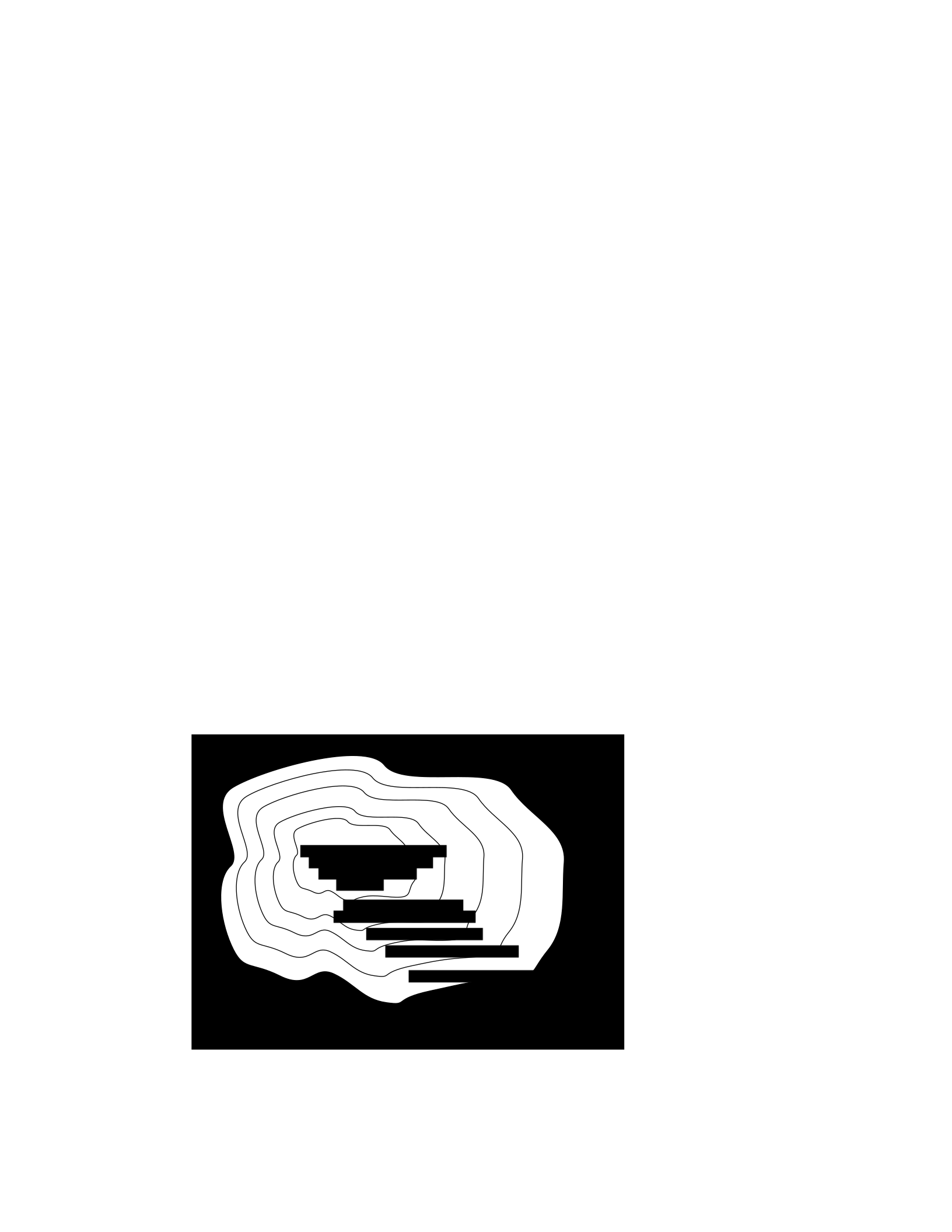
than having to re-invent the techniques yourself. And other people will be able to readily understand and
modify your designs.
We can often make a design job easier by limiting the space of possible designs, and by standardizing on:
• a basis set of primitive components;
• ways of combining the primitive components to make more complex systems;
• ways of “packaging” or abstracting pieces of a design so they can be reused (in essence creating
new “primitives”); and
• ways of capturing common patterns of abstraction (essentially, abstracting our abstractions).
Very complicated design problems can become tractable using such a primitive-combinationabstraction-
pattern (PCAP) approach. In this class, we will examine and learn to use a variety of PCAP strategies
common in EE and CS, and will even design some of our own, for special purposes. In the rest of this
section, we will hint at some of the PCAP systems we will be developing in much greater depth throughout
the class. Figure 1.1 shows one view of this development, as a successive set of restrictions of the design
space of mechanisms.
One very important thing about abstract models is that once we have fixed the abstraction, it will usually
be possible to implement it using a variety of different underlying substrates. So, as shown in figure 1.2,
we can construct general-purpose computers out of a variety of different kinds of systems, including digital
circuits and general-purpose computers. And systems satisfying the digital circuit abstraction can be
constructed from analog circuits, but also from gears or water or light.
Another demonstration of the value of abstracted models is that we can use them, by analogy, to describe
quite different systems. So, for example, the constraint models of circuits that we will study can be applied
to describing transmission of neural signals down the spinal cord, or of heat through a network of
connected bodies.
Let’s explore the abstraction hierarchy figure 1.1 in some more detail, moving up abstraction levels while
observing common patterns.
Figure 1.1 Increasingly constrained systems.
electrical systems
traditional analog circuits
digital electronic circuits
electronic computers
electronic computers
running Python programs
electronic computers with
Python programs that
select outputs by
planning

Figure 1.2 A single abstraction may have a variety of different underlying implementations.
Circuits
Typical electronics circuits are built out of a basis set of primitive components such as voltage sources,
resistors, capacitors, inductors and transistors. This set of component types was chosen to be closely
related to primitive concepts in our physical understanding of electronic systems in terms of voltage,
current, resistance, and the rate of change of those quantities over time. So, when we buy a physical
resistor, we tend to think only of its resistance; and when we buy a capacitor, we think of its ability to store
charge. But, of course, that physical resistor has some capacitance, and the capacitor, some resistance.
Still, it helps us in our designs to have devices that are as close to the ideal models as possible; and it helps
that people have been designing with these components for years, so that we can adopt the strategies
that generations of clever people have developed.
The method of combining circuit elements is to connect their terminals with conductors (wires, crimps,
solder, etc.), a process that is generically referred to as wiring. And our method of abstraction is to describe
the constraints that a circuit element exerts on the currents and voltages of terminals to which the
element is connected.
So, armed with the standard basis set of analog circuit components, we can try to build a circuit to control
our robot. We have a resistance that varies with the light level, but we need a voltage that does so, as well.
We can achieve this by using a voltage divider, which is shown in figure 1.3A. Using an abstract, constraint-
based model of the behavior of circuit components that we will
General-purpose computer
Digital circuits
T
uring
machine
Cellular
automata
Analog
electronics
Gears
Light
W
ater
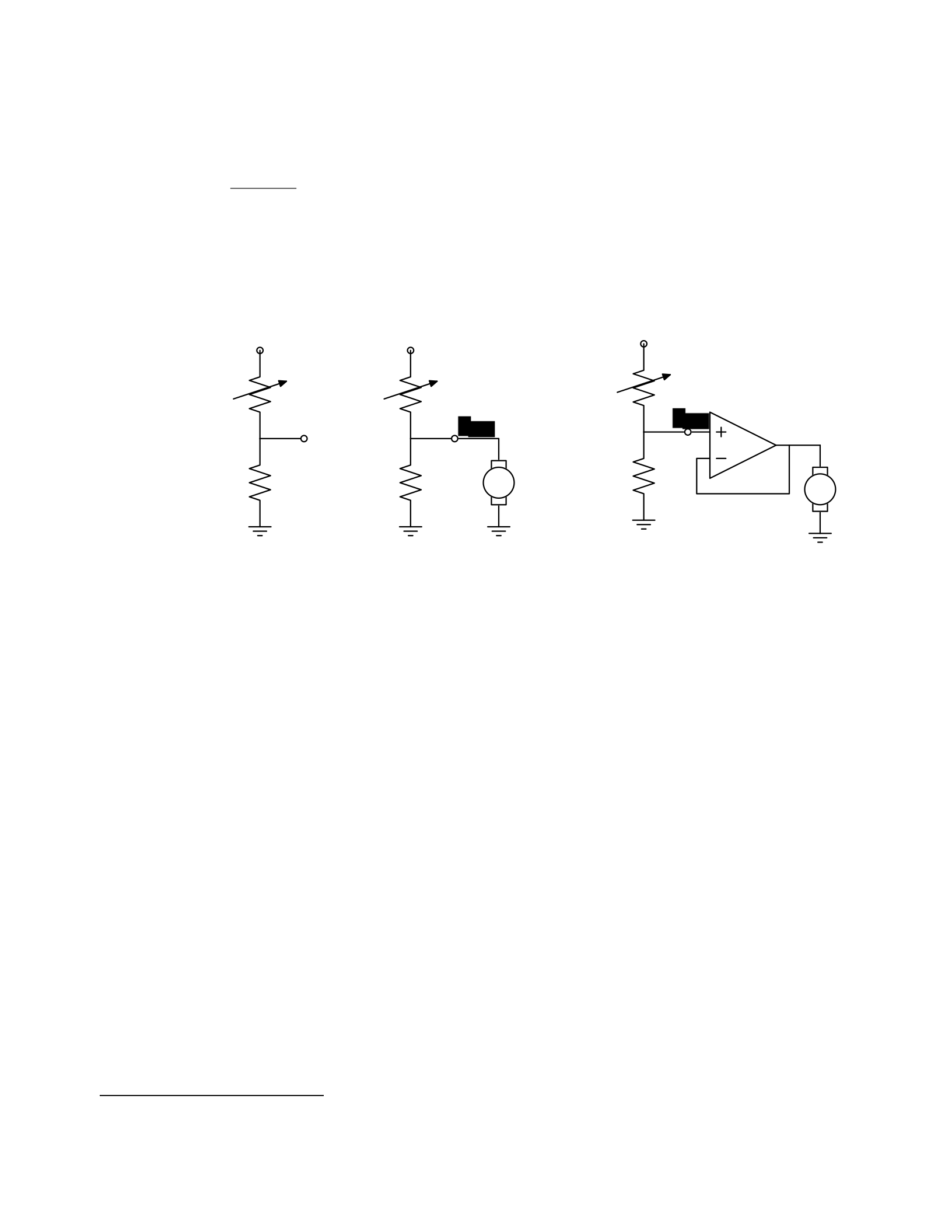
study in detail later in the course, we can determine the following relationship between Vout and Vin:
RB
Vout = Vin .
RA + RB
So, for example, if RA = RB, then Vout = Vin/2. Or, in our case, if RA actually varies with the amount of light
shining on it, then Vout will also vary with the light.
25
Vin Vin Vin
RARARA
Vout
RBRBmotor RBmotor
Figure 1.3 Voltage dividers: A. Resistor divider. B. Connected to a motor, in a way that breaks the
abstraction from part A. C. Connected to a motor, with a buffer.
That is great. So, now, we might imagine that we could use this voltage difference that we have created to
drive the motor at different speeds, depending on the light hitting the resistor, using a circuit something
like the one shown in figure 1.3B. But, sadly, that will not work. It turns out that once we connect the
motor to the circuit, it actually changes the voltages, and we can no longer maintain the voltage difference
needed to drive the motor.
So, although we have developed an abstract model of the behavior of circuit components, which lets us
analyze the behavior of a particular complete circuit design, it does not give us modularity. That is, we
cannot design two parts of a circuit, understand each of their behaviors, and then predict the behavior of
the composite system based on the behavior of the separate components. Instead, we would have to re-
analyze the joint behavior of the whole composite system. Lack of modularity makes it very difficult to
design large systems, because two different people, or the same person at two different times, cannot
design pieces and put them together without understanding the whole.
To solve this problem, we can augment our analog-circuit toolbox with some additional components that
allow us to design components with modular behavior; they “buffer” or “isolate” one part of the circuit
from another in ways that allow us to combine the parts more easily. In this class, we will use op-amps to
build buffers, which will let us solve our sample problem using a slightly more complex circuit, as shown in
figure 1.3C.
25
Do not worry if this example does not make much sense to you; we will explore this all in great detail later.

Thus, the key point is that good modules preserve abstraction barriers between the use of a module and
internal details of how they are constructed. We will see this theme recur as we discuss different PCAP
systems.
Digital circuits
In analog circuits, we think about voltages on terminals ranging over real values. This gives us the freedom
to create an enormous variety of circuits, but sometimes that freedom actually makes the design process
more difficult. To design ever more complex circuits, we can move to a much stronger, digital abstraction,
in which the voltages on the terminals are thought of as only taking on values that are either “low” or
“high” (often called 0 and 1). This PCAP system is made up of a basis set of elements, called gates, that are
built out of simpler analog circuit components, such as transistors and resistors. Adopting the digital
abstraction is a huge limitation on the kinds of circuits that can be built. However, digital circuits can be
easy to design and build and also can be inexpensive because the basic elements (gates) are simple (fewer
transisters are need to construct a gate than to construct an op amp), versatile (only a small number of
different kinds of logic elements are necessary to construct an arbitrary digital circuit), and combinations
are easy to think about (using Boolean logic). These properties allow designers to build incredibly complex
machines by designing small parts and putting them together into increasingly larger pieces. Digital
watches, calculators, and computers are all built this way.
Digital design is a very important part of EECS, and it is treated in a number of our courses at basic and
advanced levels, but is not one of the topics we will go into in detail in 6.01. Nevertheless, the same central
points that we explore in this course apply to this domain as well.
Computers
One of the most important developments in the design of digital circuits is that of the generalpurpose
“stored program” computer. Computers are a particular class of digital circuits that are general purpose:
the same actual circuit can perform (almost) any transformation between its inputs and its outputs. Which
particular transformation it performs is governed by a program, which is some settings of physical switches,
or information written on an external physical memory, such as cards or a tape, or information stored in
some sort of internal memory.
The “almost” in the previous section refers to the actual memory capacity of the computer. Exactly what
computations a computer can perform depends on the amount of memory it has; and also on the time
you are willing to wait. So, although a general-purpose computer can do anything a special-purpose digital
circuit can do, in the information-processing sense, the computer might be slower or use more power.
However, using general-purpose computers can save an enormous amount of engineering time and effort.
It is much cheaper and easier to debug and modify and manufacture software than hardware. The
modularities and abstractions that software PCAP systems give us are even more powerful than those
derived from the digital circuit abstraction.
Again, we can see how abstraction separates use from details; we don’t need to know how the circuits
inside a computer are designed, we just need to know the rules by which we can use them and the
constraints under which they perform.

Python programs
Every general-purpose computer has a different detailed design, which means that the way its program
needs to be specified is different. Furthermore, the “machine languages” for describing computer
programs, at the most primitive level, are awkward for human programmers. So, we have developed a
number of computer programming languages for specifying a desired computation. These languages are
converted into instructions in the computer’s native machine language by other computer programs,
called compilers or interpreters. One of the coolest and most powerful things about general-purpose
computers is this ability to write computer programs that process or create or modify other computer
programs.
Computer programming languages are PCAP systems. They provide primitive operations, ways of
combining them, ways of abstracting over them, and ways of capturing common abstraction patterns. We
will spend a considerable amount of time in this course studying the particular primitives, combination
mechanisms, and abstraction mechanisms made available in the Python programming language. But the
choice of Python is relatively unimportant. Virtually all modern programming languages supply a similar
set of mechanisms, and the choice of programming language is primarily a matter of taste and
convenience.
In a computer program we have both data primitives and computation primitives. At the most basic level,
computers generally store binary digits (bits) in groups of 32 or 64, called words. These words are data
primitives, and they can be interpreted by our programs as representing integers, floating-point numbers,
strings, or addresses of other data in the computer’s memory. The computational primitives supported by
most computers include numerical operations such as addition and multiplication, and locating and
extracting the contents of a memory at a given address. In Python, we will work at a level of abstraction
that does not require us to think very much about addresses of data, but it is useful to understand that
level of description, as well.
Primitive data and computation elements can be combined and abstracted in a variety of different ways,
depending on choices of programming style. We will explore these in more detail in section 1.3.2.
1.2.3 Models
So far, we have discussed a number of ways of framing the problem of designing and constructing
mechanisms. Each PCAP system is accompanied by a modeling system that lets us make mathematical
models of the systems we construct.
What is a model? It is a new system that is considerably simpler than the system being modeled, but which
captures the important aspects of the original system. We might make a physical model of an airplane to
test in a wind tunnel. It does not have to have passenger seats or landing lights; but it has to have surfaces
of the correct shape, in order to capture the important properties for this purpose. Mathematical models
can capture properties of systems that are important to us, and allow us to discover things about the
system much more conveniently than by manipulating the original system itself.
One of the hardest things about building models is deciding which aspects of the original system to model
and which ones to ignore. Many classic, dramatic engineering failures can be ascribed to failing to model
important aspects of the system. One example (which turned out to be an ethical success story, rather

than a failure) is LeMessurier’s Citicorp Building
26
, in which an engineering design change was made, but
tested in a model in which the wind came only from a limited set of directions.
Another important dimension in modeling is whether the model is deterministic or not. We might, for
example, model the effect of the robot executing a command to set its velocity as making an instantaneous
change to the commanded velocity. But, of course, there is likely to be some delay and some error. We
have to decide whether to ignore that delay and error in our model and treat it as if it were ideal; or, for
example, to make a probabilistic model of the possible results of that command. Generally speaking, the
more different the possible outcomes of a particular action or command, and the more diffuse the
probability distribution over those outcomes, the more important it is to explicitly include uncertainty in
the model.
Once we have a model, we can use it in a variety of different ways, which we explore below.
Analytical models
By far the most prevalent use of models is in analysis: Given a circuit design, what will the voltage on this
terminal be? Given a computer program, will it compute the desired answer? How long will it take? Given
a control system, implemented as a circuit or as a program, will the system stop at the right distance from
the light bulb?
Analytical tools are important. It can be hard to verify the correctness of a system by trying it in all possible
initial conditions with all possible inputs; sometimes it is easier to develop a mathematical model and then
prove a theorem about the model.
For some systems, such as pure software computations, or the addition circuitry in a calculator, it is possible
to analyze correctness or speed with just a model of the system in question. For other systems, such as
fuel injectors, it is impossible to analyze the correctness of the controller without also modeling the
environment (or “plant”) to which it is connected, and then analyzing the behavior of the coupled system
of the controller and environment.
To demonstrate some of these tradeoffs, we can do a very simple analysis of a robot moving toward a
lamp. Imagine that we arrange it so that the robot’s velocity at time t, V[t], is proportional to the difference
between the actual light level, X[t], and a desired light level (that is, the light level we expect to encounter
when the robot is the desired distance from the lamp), Xdesired ; that is, we can model our control system
with the difference equation
V[t] = k(Xdesired − X[t]) where k is the constant of proportionality, or
gain, of the controller.
Now, we need to model the world. For simplicity, we equate the light level to the robot’s position (assuming
that the units match); in addition we assume the robot’s position at time t is its position at time t−1 plus
its velocity at time t−1 (actually, this should be the product of the velocity and the length of time between
samples, but we can just assume a unit time step and thus use velocity). When we couple these models,
we get the difference equation
26
See “The Fifty-Nine Story Crisis”, The New Yorker, May 29, 1995, pp 45-53.

X[t] = X[t − 1] + k(Xdesired − X[t − 1]) .
Now, for a given value of k, we can determine how the system will behave over time, by solving the
difference equation in X.
Later in the course, we will see how easily-determined mathematical properties of a differenceequation
model can tell us whether a control system will have the desired behavior and whether or not the
controller will cause the system to oscillate. These same kinds of analyses can be applied to robot control
systems as well as to the temporal properties of voltages in a circuit, and even to problems as unrelated
as the consequences of a monetary policy decision in economics. It is important to note that treating the
system as moving in discrete time steps is an approximation to underlying continuous dynamics; it can
make models that are easier to analyze, but it requires sophisticated understanding of sampling to
understand the effects of this approximation on the correctness of the results.
Synthetic models
One goal of many people in a variety of sub-disciplines of computer science and electrical engineering is
automatic synthesis of systems from formal descriptions of their desired behavior. For example, you might
describe some properties you would want the input/output behavior of a circuit or computer program to
have, and then have a computer system discover a circuit or program with the desired property.
This is a well-specified problem, but generally the search space of possible circuits or programs is much
too large for an automated process; the intuition and previous experience of an expert human designer
cannot yet be matched by computational search methods.
However, humans use informal models of systems for synthesis. The documentation of a software library,
which describes the function of the various procedures, serves as an informal model that a programmer
can use to assemble those components to build new, complex systems.
Internal models
As we wish to build more and more complex systems with software programs as controllers, we find that
it is often useful to build additional layers of abstraction on top of the one provided by a generic
programming language. This is particularly true when the nature of the exact computation required
depends considerably on information that is only received during the execution of the system.
Consider, for example, an automated taxi robot (or, more prosaically, the navigation system in your new
car). It takes, as input, a current location in the city and a goal location, and gives, as output, a path from
the current location to the goal. It has a map built into it.
It is theoretically possible to build an enormous digital circuit or computer program that contains a look-
up table, in which we precompute the path for all pairs of locations and store them away. Then when we
want to find a path, we could simply look in the table at the location corresponding to the start and goal
location and retrieve the precomputed path. Unfortunately, the size of that table is too huge to
contemplate. Instead, what we do is construct an abstraction of the problem as one of finding a path from
any start state to any goal state, through a graph (an abstract mathematical construct of “nodes” with
“arcs” connecting them). We can develop and implement a general-purpose algorithm that will solve any
shortest-path problem in a graph. That algorithm and implementation will be useful for a wide variety of

possible problems. And for the navigation system, all we have to do is represent the map as a graph, specify
the start and goal states, and call the general graph-search algorithm.
We can think of this process as actually putting a model of the system’s interactions with the world inside
the controller; it can consider different courses of action in the world and pick the one that is the best
according to some criterion.
Another example of using internal models is when the system has some significant lack of information
about the state of the environment. In such situations, it may be appropriate to explicitly model the set of
possible states of the external world and their associated probabilities, and to update this model over time
as new evidence is gathered. We will pursue an example of this approach near the end of the course.
1.3 Programming embedded systems
There are many different ways of thinking about modularity and abstraction for software. Different models
will make some things easier to say and do and others more difficult, making different models appropriate
for different tasks. In the following sections, we explore different strategies for building software systems
that interact with an external environment, and then different strategies for specifying the purely
computational part of a system.
1.3.1 Interacting with the environment
Increasingly, computer systems need to interact with the world around them, receiving information about
the external world, and taking actions to affect the world. Furthermore, the world is dynamic, so that as
the system is computing, the world is changing, requiring future computation to adapt to the new state of
the world.
There are a variety of different ways to organize computations that interact with an external world.
Generally speaking, such a computation needs to:
37. get information from sensors (light sensors, sonars, mouse, keyboard, etc.),
38. perform computation, remembering some of the results, and
39. take actions to change the outside world (move the robot, print, draw, etc.).
These operations can be put together in different styles.
1.3.1.1 Sequential
The most immediately straightforward style for constructing a program that interacts with the world is the
basic imperative style, in which the program gives a sequence of ’commands’ to the system it is controlling.
A library of special procedures is defined, some of which read information from the sensors and others of
which cause actions to be performed. Example procedures might move a robot forward a fixed distance,
or send a file out over the network, or move video-game characters on the screen.
In this model, we could naturally write a program that moves an idealized robot in a square, if there is
space in front of it.
if noObstacleInFront: moveDistance(1)
turnAngle(90) moveDistance(1)
turnAngle(90) moveDistance(1)

turnAngle(90) moveDistance(1)
turnAngle(90)
The major problem with this style of programming is that the programmer has to remember to check the
sensors sufficiently frequently. For instance, if the robot checks for free space in front, and then starts
moving, it might turn out that a subsequent sensor reading will show that there is something in front of
the robot, either because someone walked in front of it or because the previous reading was erroneous.
It is hard to have the discipline, as a programmer, to remember to keep checking the sensor conditions
frequently enough, and the resulting programs can be quite difficult to read and understand.
For the robot moving toward the light, we might write a program like this:
while lightValue < desiredValue:
moveDistance(0.1)
This would have the robot creep up, step by step, toward the light. We might want to modify it so that the
robot moved a distance that was related to the difference between the current and desired light values.
However, if it takes larger steps, then during the time that it is moving it will not be sensitive to possible
changes in the light value and cannot react immediately to them.
1.3.1.2 Event-Driven
User-interface programs are often best organized differently, as event-driven (also called interrupt driven)
programs. In this case, the program is specified as a collection of procedures (called ’handlers’ or
’callbacks’) that are attached to particular events that can take place. So, for example, there might be
procedures that are called when the mouse is clicked on each button in the interface, when the user types
into a text field, or when the temperature of a reactor gets too high. An “event loop” runs continuously,
checking to see whether any of the triggering events have happened, and, if they have, calling the
associated procedure.
In our simple example, we might imagine writing a program that told the robot to drive forward by default;
and then install an event handler that says that if the light level reaches the desired value, it should stop.
This program would be reactive to sudden changes in the environment.
As the number and frequency of the conditions that need responses increases, it can be difficult to both
keep a program like this running well and guarantee a minimum response time to any event.
1.3.1.3 Transducer
An alternative view is that programming a system that interacts with an external world is like building a
transducer with internal state. Think of a transducer as a processing box that runs continuously. At regular
intervals (perhaps many times per second), the transducer reads all of the sensors, does a small amount
of computation, stores some values it will need for the next computation, and then generates output
values for the actions.
This computation happens over and over and over again. Complex behavior can arise out of the temporal
pattern of inputs and outputs. So, for example, a robot might try to move forward without hitting
something by defining a procedure:

def step(): distToFront = min(frontSonarReadings) motorOutput(gain *
(distToFront - desiredDistance), 0.0)
Executed repeatedly, this program will automatically modulate the robot’s speed to be proportional to the
free space in front of it.
The main problem with the transducer approach is that it can be difficult to do tasks that are fundamentally
sequential (like the example of driving in a square, shown above). We will start with the transducer model,
and then, as described in section 4.3, we will build a new abstraction layer on top of it that will make it
easy to do sequential commands, as well.
1.3.2 Programming models
Just as there are different strategies for organizing entire software systems, there are different strategies
for formally expressing computational processes within those structures.
1.3.2.1 Imperative computation
Most of you have probably been exposed to an imperative model of computer programming, in which we
think of programs as giving a sequential set of instructions to the computer to do something. And, in fact,
that is how the internals of the processors of computers are typically structured. So, in Java or C or C++,
you write typically procedures that consist of lists of instructions to the computer:
49. Put this value in this variable
50. Square the variable
51. Divide it by pi
52. If the result is greater than 1, return the result
In this model of computation, the primitive computational elements are basic arithmetic operations and
assignment statements. We can combine the elements using sequences of statements, and control
structures such as if, for, and while. We can abstract away from the details of a computation by defining
a procedure that does it. Now, the engineer only needs to know the specifications of the procedure, but
not the implementation details, in order to use it.
1.3.2.2 Functional computation
Another style of programming is the functional style. In this model, we gain power through function calls.
Rather than telling the computer to do things, we ask it questions: What is 4 + 5? What is the square root
of 6? What is the largest element of the list?
These questions can all be expressed as asking for the value of a function applied to some arguments. But
where do the functions come from? The answer is, from other functions. We start with some set of basic
functions (like “plus”), and use them to construct more complex functions.
This method would not be powerful without the mechanisms of conditional evaluation and recursion.
Conditional functions ask one question under some conditions and another question under other
conditions. Recursion is a mechanism that lets the definition of a function refer to the function being
defined. Recursion is as powerful as iteration.

In this model of computation, the primitive computational elements are typically basic arithmetic and list
operations. We combine elements using function composition (using the output of one function as the
input to another), if, and recursion. We use function definition as a method of abstraction, and the idea of
higher-order functions (passing functions as arguments to other functions) as a way of capturing common
high-level patterns.
1.3.2.3 Data structures
In either style of asking the computer to do work for us, we have another kind of modularity and
abstraction, which is centered around the organization of data.
At the most primitive level, computers operate on collections of (usually 32 or 64) bits. We can interpret
such a collection of bits as representing different things: a positive integer, a signed integer, a floating-point
number, a Boolean value (true or false), one or more characters, or an address of some other data in the
memory of the computer. Python gives us the ability to work directly with all of these primitives, except
for addresses.
There is only so much you can do with a single number, though. We would like to build computer programs
that operate on representations of documents or maps or circuits or social networks. To do so, we need to
aggregate primitive data elements into more complex data structures. These can include lists, arrays,
dictionaries, and other structures of our own devising.
Here, again, we gain the power of abstraction. We can write programs that do operations on a data
structure representing a social network, for example, without having to worry about the details of how the
social network is represented in terms of bits in the machine.
1.3.2.4 Object-oriented programming: computation + data structures
Object-oriented programming is a style that applies the ideas of modularity and abstraction to execution
and data at the same time.
An object is a data structure, together with a set of procedures that operate on the data. Basic procedures
can be written in an imperative or a functional style, but ultimately there is imperative assignment to state
variables in the object.
One major new type of abstraction in OO programming is “generic” programming. It might be that all
objects have a procedure called print associated with them. So, we can ask any object to print itself,
without having to know how it is implemented. Or, in a graphics system, we might have a variety of
different objects that know their x,y positions on the screen. So each of them can be asked, in the same
way, to say what their position is, even though they might be represented very differently inside the
objects.
In addition, most object-oriented systems support inheritance, which is a way to make new kinds of objects
by saying that they are mostly like another kind of object, but with some exceptions.
This is another way to take advantage of abstraction.

Programming languages
Python as well as other modern programming languages, such as Java, Ruby and C++, support all of these
programming models. The programmer needs to choose which programming model best suits the task.
This is an issue that we will return to throughout the course.
1.4 Summary
We hope that this course will give you a rich set of conceptual tools and practical techniques, as well as an
appreciation of how math, modeling, and implementation can work together to enable the design and
analysis of complex computational systems that interact with the world.
Acknowledgments
Thanks to Jacob White, Hal Abelson, Tomas Lozano-Perez, Sarah Finney, Sari Canelake, Eric Grimson, Ike
Chuang, and Berthold Horn for useful comments and criticisms, and to Denny
Freeman for significant parts and most of the figures in the linear systems chapter. - LPK

