


PATCH-BASED OPTIMIZATION AND CURRICULUM LEARNING:
IMPROVING DEEP LEARNING EFFICIENCY AND MODEL SECURITY
CHAPTER I
INTRODUCTION
Deep Learning (DL) algorithms have consistently made remarkable progress across a
range of tasks [1], [2], [3]. The ongoing evolution of Deep Neural Network (DNN) architectures
has been extraordinary, showing significant improvements with each iteration driving
advancements in a variety of practical field [4], [5], [6], [7], [8]. One prominent example of these
architectures is the Convolutional Neural Network (CNN) [5], [7], [9]. Notably, CNNs, trained
on images for classification and detection tasks, have outperformed human capabilities in several
visual challenges such as image classification, face recognition [10], [11], and speech
recognition [12].
Despite significant progress in developing these models, architectures, and learning
algorithms, our understanding of their optimization processes and internal structures—
particularly for CNNs and DNNs—remains limited [13]. Often, DL trained models are perceived
as 'black boxes' [14] whose inner workings of which are hard to decipher. This limited
understanding presents several key challenges, including:
•An increased vulnerability to adversarial attacks [15];
•The necessity for vast amounts of labeled data to achieve desirable performance,
•Computational resource requirements that scale up proportionately with the volume of
data.

Beyond these limitations, recent research has revealed several surprising properties of
CNNs, particularly when compared to human visual recognition capabilities. An outcome
highlighted in Szegedy et al. [15] is that a network trained for object recognition tasks that
achieves high generalization performance could easily be misled by minor perturbations on an
input that it would otherwise recognize. Remarkably, in various settings, the number of altered
pixels is statistically insignificant relative to the image's total pixel count and nearly undetectable
to the human eye. Moreover, Nguyen et al [16] demonstrated that such networks could exhibit
complete certainty in their classification of an image that humans would dismiss as mere noise
(see Figure 1.2. (right) for an illustration). Furthermore, Zhang et al. [17] reported that deep
networks could readily approximate pure noise without any difficulty.
These findings suggest that the representations learned by DNNs differ fundamentally
from the cognitive processes employed for image analysis. Given these insights, the dissertation
centered around the following research questions to formulate training and preprocessing
algorithms:
•How did the features in the training set, recognizable by humans, influence the
learnability of a task?
of those images for CNNs?
•Was it feasible to preprocess the training set or feature maps in a way that does not
preserve feature locality but enhances learning efficiency, improves generalization, and
counters adversarial attacks?
•Could we modulate the convolution filtering on individual images to produce more
important feature maps?
•Were there strategies to be conceived that leverage the distinct attributes of images for
enhanced learning?

We developed a framework, termed Deep-CLO, to elucidate correlations between training
samples and network performance, taking full advantage of CNNs' capacity as universal
approximators [18]. This trait allows CNNs to model any data, empowering our training and
preprocessing algorithms. Deep-CLO uniquely integrates curriculum learning (CL) into the deep
learning training process. CL, as introduced by Bengio et al. [19], is a methodology where
training samples are sequentially supplied based on a specific ranking system. Additionally,
Deep-CLO introduces a novel algorithm, PROSIS (Patch Reordering Optimization for Structured
Input Sequencing). This algorithm is designed to optimize training and amplify feature extraction
by preprocessing training samples both in 2D and 3D spaces.
Dissertation Contributions
With the rapid proliferation of image-based data, it becomes imperative to devise methods
that not only enhance the performance of CNNs but also ensure that they're robust against
adversarial attacks and require less data for training to achieve reasonable performance. The
contributions outlined in this dissertation are a culmination of efforts aimed at addressing some
of these issues. By focusing on the structure, arrangement, and presentation of the training data,
we've endeavored to tap into the innate potential of CNNs and harness their strengths more
effectively.
Patch Reordering Optimization for Structured Input Sequencing
We formulated two preprocessing algorithms that strategically rearrange image patches
within a dataset to optimize CNN performance. An image patch (image region, or slice) is
defined as a contiguous group of pixels within a sample. Our methods prioritize organizing these
patches based on specific measures. Our findings revealed that this patch-based arrangement
accelerates the training convergence and enhances both the generalization capabilities and
adversarial robustness of select models [20]. Additionally, this algorithm enriches the dataset
while preserving its integrity. Furthermore, this technique enriches the dataset without
compromising its integrity. We hypothesize that using this preprocessing method enables CNNs

to detect and leverage features that strengthen their defense against pixel-based adversarial
attacks.
Curriculum Learning
Our Deep-CLO framework offers an enhanced approach to curriculum learning (CL).
Within this framework, we devised a series of algorithms specifically for the strategic selection
of curriculum learning schemes (syllabi). These algorithms leverage metrics to mathematically
quantify dependencies among training samples. Drawing inspiration from human learning where
concepts are systematically organized, CL differs from conventional training methods that
randomly present samples. Instead, it orders the training set from the simplest to the most
challenging, as posited by Bengio et al. [19]. This dissertation delved deeper into CL and
introduced groundbreaking, practical techniques that aim to popularize CL. We presented
methods for ranking samples based on information-theoretic and statistical assessments of
relationships between adjacent inputs. Our results underline the efficiency of these techniques,
showcasing faster convergence compared to traditional training approaches (Ghebrechristos &
Alaghband, 2019, 2020; Henok Ghebrechristos, Gita Alaghband, 2019). With these
advancements, this dissertation makes significant contribution in making curriculum learning a
practical and integral component of future deep learning pipelines.
Application-Focused Contributions
Deep-CLO offers an intuitive approach by prioritizing the learning sequence of data,
ensuring that models extract maximal information from available data, even when limited
amount. This structured approach to learning harnesses the inherent characteristics of the data,
producing models with satisfactory generalization capabilities.
Combined, these algorithms also allow models to be robust against adversary attacks.
Through preprocessing and training techniques, we can achieve reasonable performance from
models even when they are subjected to localized adversary attacks, ensuring that the challenge
of adversary attacks does not impede the progress and application of deep learning.

Limitations and Future Work
Given the ever-evolving landscape of deep learning, the findings in this dissertation
should be viewed in the context of the technology and understanding available as of the time of
the research. Future work will aim to extend the methods developed here and further explore the
potential of our framework to improve other areas of deep learning.
Dissertation Outline
The remaining content is organized into several cohesive sections, each presenting an
essential component of our work. Chapter 2 establishes the foundational concepts in deep
learning and CNNs. Chapter 3 provides a literature review of pertinent research directly related
to this dissertation. Chapter 4 delves into the practical side, detailing the development and
implementation of our framework. Chapter 5 rigorously tests and evaluates our proposed
algorithms, while Chapter 6 presents the application and experimental results of PROSIS
algorithm in enhancing CNN. Chapter 7 ventures further, exploring the application of PROSIS
for 3D convolution and adversarial attacks. The dissertation closes with a detailed bibliography.
CHAPTER 2
RESEARCH BACKGROUND AND FUNDAMENTAL CONCEPTS
Introduction
This chapter aims to provide a thorough grounding in the foundational concepts integral
to understanding the research presented in this dissertation. We first present fundamentals of deep
learning, specifically focusing on CNNs, their architecture, and their performance in image
classification tasks. Next, we explore the internal mechanics of CNNs, explaining the learning

process including the crucial roles of forward and backpropagation algorithms and various
optimization methods.
Following that we present an information-theoretic interpretation of CNNs and their
universal approximation property. This is done to illuminate the theoretical potential of CNNs to
model any type of data. We then pivot to the inherent vulnerabilities and limitations of CNNs,
encompassing susceptibility to adversarial attacks.
In the subsequent section, we introduce the concept of Curriculum Learning (CL) for
CNNs, highlighting its benefits and contrasting it with traditional machine learning approaches.
Following this, we introduce the methodological shift of interpreting images as two-dimensional
random variables, a foundational premise that enables the application of information-theoretic
methodologies to refine the curriculum learning dynamics for CNNs.
Deep Learning
As depicted in Figure 2.1, Deep Learning (DL) is a subset of machine learning, loosely
premised on the conceptual workings of the human brain [24]. It employs a category of
algorithms known as artificial neural networks (ANNs, Figure 2.2. ), which are complex
computational models designed to simulate the way neurons operate within the brain. More
specifically, these models are often referred to as feedforward neural networks or multilayer
perceptron (MLPs) due to their structured and layered architecture.
The layered structure of these networks is a pivotal component of their functionality [25].
Each layer is made up of an assembly of interconnected nodes, informally known as neurons,
which are mathematical analogues to the biological neurons found within a brain. These neurons
interact with each other, transmitting and processing information in a manner akin to their
biological counterparts [26].
The hidden layers enable the ANNs to learn hierarchically, with each layer extracting and
refining features from the input data. The lower layers often learn to recognize simple patterns,
while the higher layers combine these simple patterns to recognize more complex structures. For

example, in an image recognition task, the lower layers may recognize lines and edges,
intermediate layers may recognize shapes or textures, and the higher layers may recognize
complex objects like faces or specific items [27].
Learning Objective of ANNs
The primary goal of a neural network is to learn a function or a mapping 𝑓that can
accurately map inputs to their corresponding outputs [28]. This is achieved by iteratively learning
the optimal set of parameters (weights and biases) that minimize a defined loss function.
Mathematically, given an input vector 𝑥, the learning objective is to find an optimal set of
parameters 𝜃 for the function 𝑓(𝑥; 𝜃) to accurately predict the corresponding output 𝑦 [28].
For example, in a cat vs. dog image classifier model, 𝑦 = 𝑓(𝑥) maps an input image 𝑥
to its category y. The training process aims to find the optimal set of parameters 𝜃, that minimize
the difference between the predicted outputs 𝑓(𝑥) and the actual outputs (labels) 𝑦 for all
samples in a training dataset 𝐷 [29]. This difference is often quantified using a loss function
𝐿(𝑦, 𝑓(𝑥; 𝜃)). In other words, the learning objective can be seen as an optimization problem,
where we seek to find:
𝜃∗ = 𝑎𝑟𝑔𝑚𝑖𝑛 ‘ 𝐿(𝑦, 𝑓(𝑥;
𝜃)).
(2. 1)
*+
In this context, the function 𝑓 represents the structure of the neural network - its
architecture, the activation functions, etc. – and 𝜃 stands for the learned parameters of the
function. The form of the loss function 𝐿 depends on the task at hand and the specific network
architecture. One of the common methods used to find the optimal parameters that minimize the
loss function is called Stochastic Gradient Descent (SGD) [30]. SGD iteratively adjusts the

parameters in the direction that most reduces the value of the loss function, using a fraction of the
training data (a batch 𝐵) to compute the gradient at each step [30]. This iterative optimization
process continues until a stopping condition is met, which could be a predefined number of
iterations (epochs) or the point at which further training does not significantly reduce the loss
[31]. Details of this optimization algorithm and its variant techniques are discussed below.
Deep Neural Network Architectures
Artificial Neural Networks (ANNs) come in a variety of types, each characterized by
unique architecture and areas of applicability [4], [21], [28], [29], [31], [32], [33], [34], [35],
[36], [37], [38]. Notable among these are Recurrent Neural Networks (RNNs) [39], Transformers
[38], and Generative Adversarial Networks (GANs) [28]. We will briefly describe these
architectures in the subsequent sections to give the reader a basic understanding. However, the
focus of this dissertation is on CNNs, an architecture highly suited to tasks involving image data.
As such, a detailed exploration of CNNs will be presented in its own dedicated section.
Feed Forward Networks (FNNs)
As one of the simplest types of artificial neural networks, Feedforward Neural Networks
(FNNs, Figure 2.3. ) stand as the basis from which more complex network architectures have
evolved [40]. In FNNs, information moves in one direction only, from the input layer to the
output layer, without looping back, hence the term 'feedforward'.
A key characteristic of FNNs is that they are acyclic - there are no feedback connections
in which outputs of the network are fed back into itself. This acyclic nature results in the absence
of an internal state within the network. As such, FNNs are ill-suited for processing temporal or
sequential data as they do not possess the capability to remember past inputs [32]. Therefore,
FNNs are typically employed in scenarios where the input-output mapping is fixed, such as in
image recognition tasks where the input (image) directly leads to an output (classification) [5].

Despite their simplicity, FNNs can model complex non-linear relationships given a
sufficient number of neurons in the hidden layers, thus forming the foundational building block
of deep learning [18]. Furthermore, the straightforward architecture and absence of feedback
connections result in models that are easier to understand and interpret compared to their more
complex counterparts like RNNs and CNNs [41].
Recurrent Neural Networks (RNNs)
RNNs are a distinct class of neural networks specifically designed to process sequential
data [39]. The architecture of RNNs, depicted in Figure 2.4. permits them to have an internal
memory, capturing and utilizing information from previous inputs in a sequence to inform the
current state [39]. This characteristic lends RNNs their unique capability to handle tasks where
temporal dependencies between inputs are critical.
RNNs are widely used in applications involving sequence-to-sequence tasks, where the
order of data points plays a vital role. Examples of such tasks include natural language
processing (NLP) [42] (e.g., text translation [43], sentiment aalysis [44], language modeling
[45]), speech recognition [12], and time-series analysis (e.g., stock price prediction ( [46])),
weather forecasting [47]) .
In language modeling [45], RNNs can be used as predictive models of language where
the prediction of the next word in a sentence depends not just on the immediate previous word,
but on a context that includes words prior to it in the sentence. Similarly, in time-series prediction
tasks like weather forecasting [47], the future state of the weather is not only influenced by the
immediate past but can also be affected by weather patterns over preceding days or weeks. By
maintaining an internal state, RNNs can capture these time dependencies.
In speech recognition, RNNs can handle variable length inputs and outputs, making them
suitable for tasks such as transcription where the length of the spoken word sequence and the
corresponding text can differ. Also, in the music generation, RNN can learn patterns over
different time scales, from individual notes to motifs to larger musical structures.

To deal with video data, which can be seen as a sequence of frames, RNNs can be
employed to analyze the temporal dynamics between frames for applications like activity
recognition [48], where the context and order of frames are important to identify the performed
activities accurately.
Transformer Networks
Since their introduction in 2017 [49], Transformers have revolutionized the field of NLP
and have found their way to other application domains. The unique architecture of transformers,
Figure 2.5. , relies on a mechanism known as self-attention [49] which allows the model to
weigh the importance of tokens (like words in a sentence) relative to other tokens. This is
essential for tasks where understanding context and relationship between words is important.
architectures that have been proposed since their introduction, such as Bidirectional Encoder
Representations from Transformers (BERT) [38], Generative Pretrained Transformer (GPT)
(Radford et al.), Text-to-Text Transfer Transformer (T5) [51], and many others [52]. These
models have set new performance benchmarks on a variety of NLP tasks, including but not
limited to machine translation, sentence classification, sentiment analysis, and language
modeling.
In recent years, transformers have also been adapted for use with non-textual data, such as
images [53] and graphs [54], demonstrating their versatility and the potential for wide-ranging
applications. However, it is important to note that the computational and memory requirements
for training transformer models, particularly on large datasets, can be quite substantial, which is a
topic of ongoing research [55].
Generative Adversarial Networks
Generative Adversarial Network (GAN)s, introduced by Goodfellow et al. in 2014 [28],
are a type of neural network architectures that are primarily used for generating new data. As
depicted in Figure 2.6, GAN consists of two neural networks: a generator and a discriminator.

During training, the generator creates new data instances, while the discriminator evaluates the
generated data for authenticity. Both the generator and the discriminator are trained
distinguish from real data. GANs have shown impressive results in generating realistic images
[28], music [56], speech [57], and text [58]. In recent years, GANs have been used in diverse
applications including image synthesis [28], semantic image editing [59], style transfer [60],
image super-resolution [61] and classification [62].
Convolutional Neural Networks
Convolutional Networks (CNN)s, known for their success in image recognition, typically
comprise a series of feature extraction and classification stages (Figure 2.7. ). During each stage,
it employs several layers, each containing tens of thousands of neurons. The feature extraction
stages are primarily composed of convolutional and pooling layers [32]. In a convolutional layer,
each neuron representing a filter is connected to a small patch of a feature map from the previous
layer through a set of weights. The result of the weighted sum is then passed through an
activation function that performs non-linear transformation and prevents learning trivial linear
combinations of the inputs. The pooling layers are used to reduce computation time by
subsampling from convolution outputs and to gradually buildup further spatial invariance [63]. In
the following sections, we delve into these and other fundamental components of CNNs, their
architecture, how they are trained, their applications, and the challenges they present, offering a
comprehensive understanding of their role in deep learning. A thorough understanding of CNNs
forms the backbone of this dissertation and will be instrumental in the discussions to follow.
CNN Architecture
The essential layers in a CNN include input, convolution, activation, pooling, fully
connected, and output layers. At its core, the architecture of a CNN is characterized by a
sequence of these layers, each serving a distinct purpose.

Input Layer and Digital Images
The input layer, being the first layer of any neural network, acts as the interface between
the raw data (images) and the remaining structure of the model. For CNNs, the data fed into the
input layer is usually in the form of multi-dimensional array or tensor, which represent images
[63]. Formally, the input layer can be described in terms of the dimensions of the image being
processed [5]. Below we discuss three distinct types of inputs commonly used; grayscale image,
color image and volumetric data [64].
A digital image is a numerical representation of a visual image, encoded as a set of
discrete values [65]. At the most basic level, an image is represented as a tensor,
𝑥 ∈ ℝ,
× / × 0 × 1,
(2. 2)
where H denotes the height of the image, W denotes the width of the image, C denotes the
number of color channels, and Z denotes the depth dimension.
The input layer receives this tensor representation of an image and initiates the process of
feature extraction and abstraction. For a grayscale image, both C and Z are equal to 1. The input
layer can be represented as a 2D tensor 𝑥 ∈ 𝑅, × / [29]. Each element of the tensor,
𝑥(𝑖, 𝑗), stands for the intensity of pixel at the i-th row and j-th column of the image. A colored
image is represented in the Red-Green-Blue (RGB) format. The input layer therefore encodes the
input image as a 3D tensor 𝑥 ∈ 𝑅, × /× 1 where 𝐶signifies the number of
color channels (3 for RGB images) [5]. Similarly, each element 𝑥(𝑖, 𝑗, 𝑘), denotes the intensity
of the k-th color channel of the pixel positioned at the i-th row and j-th column of the image.
When dealing with volumetric data, such as 3D medical imaging data (CT, MRI), the input
becomes a 4D tensor 𝑥 ∈ 𝑅, × /× 0 × 1 [66].
Convolutional Layers and Discrete Convolution
At the heart of CNN is a Convolution Layer [32]. This layer performs a series of
convolution operations on the input data to extract essential features. Discrete image convolution,
an extension of the general mathematical convolution, is used to extract patterns from training
samples [63].
Mathematics of Convolution
Given two continuous functions f and 𝑔, the convolution operation ⊛ is defined as:
2j 𝑓 𝑑𝜏
(2. 3)
32
When it is applied in the continuous domain, the result expresses the overlap of the function 𝑓 as
it is shifted over 𝑔 [67]. Here, 𝑡is a variable denoting time, and 𝜏 is a dummy variable that
represents the time delay in the function 𝑔 relative to 𝑓. The operation 𝑡 − 𝜏 in the
argument of 𝑔 represents this delay.
In the context of CNNs, this is modified to be a discrete operation between a section of an
image 𝐼 and kernel (or filter) matrix 𝐾 (Figure 2.8) [8] .
834 %34
‘ ‘ 𝐼(𝑢 − 𝑖, 𝑣 − 𝑗)𝐾(𝑖, 𝑗),
(2. 4) 967 567
dimensions respectively.

Convolution at a given layer is applied to the output of the previous layer, except for the
first convolutional layer where the operation is applied directly to the input image. As the kernel
moves across the entire image, this operation is repeated, and an entire feature map (𝑓𝑚) is
constructed, representing the convolved image. For a given layer 𝑙, the input comprises (𝑓𝑚)"’34
feature maps from the previous layer [32]. When 𝑙 = 1, the input is a single image consisting of
one or more channels. The output of layer 𝑙 consists of (𝑓𝑚)4" feature maps.
Feature Maps
Feature map is output of a convolution operation. As depicted in Figure 2.8 and Figure
2.9, feature map is a spatially reduced version of the original input, but with the features
highlighted by the filter. They are considered encodings of features and their locations present in
the input [63]. If the network is trained correctly, these highlighted features are instrumental in
helping the network make its final decision [27].
The kernel – usually having fixed dimensions that are significantly smaller than the input
– applied to the input to generate a feature map. The 𝑖&: fm of a given layer 𝑙, represented
𝑓𝑚9" is computed as
8("#$)
𝑓𝑚9" = 𝐵9" + ‘ 𝐾9",5 ∗ 𝑓𝑚5"34,
(2. 5)
564
where 𝑚("34)is the total number of feature maps generated by the previous layer, 𝐵9" is a bias
matrix and 𝐾9",5 is a filter connecting the 𝑗&: feature map in layer 𝑙 [63]. The trainable weights
are found in the filters 𝐾9",5 and the bias matrices 𝐵9".
Pooling Layers

Pooling layers, which commonly follow the convolutional layers, are primarily used to
reduce the spatial dimensions (height and width) of the input. This dimensionality reduction
helps not only to reduce the computation load and the model's complexity but also to control
overfitting [63].
The mechanics of pooling involve sweeping a filter (often referred to as pooling window)
𝑊 across the input feature map (Figure 2.9). For each position the filter covers, it computes a
single value as the output. The way this value is computed depends on the type of pooling
operation used. In a standard pooling operation, the filter slides over the input feature map in a
the filter moves at each step. However, unlike the convolution operation, pooling does not use
any weights or learnable parameters. Instead, it applies a simple aggregation function, such as
taking the maximum value within the filter region [68].
There are several types of pooling operations, each having unique characteristics. Below
we discuss a few commonly used in CNNs.
Max Pooling
Max pooling [63] is the most used pooling technique. It calculates the maximum value in
a window (patch) of each feature map. The operation can be mathematically represented as:
𝑓(𝑥95) = 𝑚𝑎𝑥(8,%)∈ /&’ 𝑥8% ,
(2. 6)
where 𝑾𝒊𝒋 represents the pooling window in the input centered at location 𝒊, 𝒋 and 𝒙𝒎𝒏 are the
pixel intensities in the window.
Average Pooling
Average pooling [63] calculates the average value for each patch on the input feature map.
The operation can be expressed as:
1
𝑓(𝑥95) = ‘ 𝑥8% ,

(2. 7) y𝑊95y(8,%)∈ /&’
where y𝑊95y is the number of pixels in the pooling window 𝑊95.
Sum Pooling
Sum Pooling computes the sum of all pixel intensities within the pooling window. The
mathematical representation is like Average Pooling, without the division by the number of
elements: 𝑓 ‘ 𝑥8% .
(2. 8)
(8,%)∈ /&’
Global Max Pooling and Global Average Pooling
These operations apply pooling to the entire feature map [69]. For Global Max Pooling,
the output is the maximum pixel intensity value in the entire feature map. For Global Average
Pooling, the output is the average pixel intensity value in the feature map.
RoI (Region of Interest) Pooling
RoI pooling [70] is used in object detection tasks to convert regions of any size into a
fixed size. The ROI pooling process involves taking a section of the input feature map that
corresponds to a Region of Interest and applying a pooling operation (usually max pooling) to
convert that section into a fixed size. This allows the network to process inputs of different sizes
and aspect ratios.
Fully Connected Layer
After several rounds of convolution and pooling, the high-level reasoning in the neural
network happens in the Fully Connected (FC) Layers. Also known as the Dense Layer, this layer
is responsible for classifying the features extracted by the previous layers. Each neuron in a fully

connected layer is connected to every neuron in the previous layer, hence the name "fully
connected" [63].
Its function is to flatten the high-level features learned from the previous layers into a
single long continuous linear vector, which is used as input for the final classification part of the
network [64]. Formally, if we denote the input vector to FC layer as 𝑋F, the output 𝑦 can be
represented as:
𝑦 = 𝑓(𝑊𝑋F + 𝑏)
(2. 9)
where:
•𝑊 is the weight matrix containing the learned weights connecting the neurons from the
previous layer (output of the last pooling or convolutional layer) to the neurons in the
fully connected layer.
•𝑏 is the bias vector.
•𝑓is an activation function such as the Rectified Linear Unit (ReLU) or the Softmax
function [71].
The weights and biases in the fully connected layers, just like in convolutional layers, are
learned through the backpropagation algorithm and stochastic gradient descent or its variants
during the training phase [72]. These layers essentially perform high-level reasoning such as
classification based on the features extracted by the previous layers.
The last fully connected layer in the CNN architecture usually employs the Softmax
activation function, which provides a set of output values between 0 and 1 that sum to 1 [29].
These values are essentially the probabilities of the input image belonging to one of the classes
the network is trained to identify.

The fully connected layers are a crucial component of the CNN architecture as they map
the learned high-dimensional features onto the final classification labels. However, they also
contribute most of the parameters to the network, leading to challenges such as overfitting, which
are addressed through strategies like regularization and dropout [73].
Activation Functions
Another integral component of CNNs, as well as other types of ANN architectures, is the
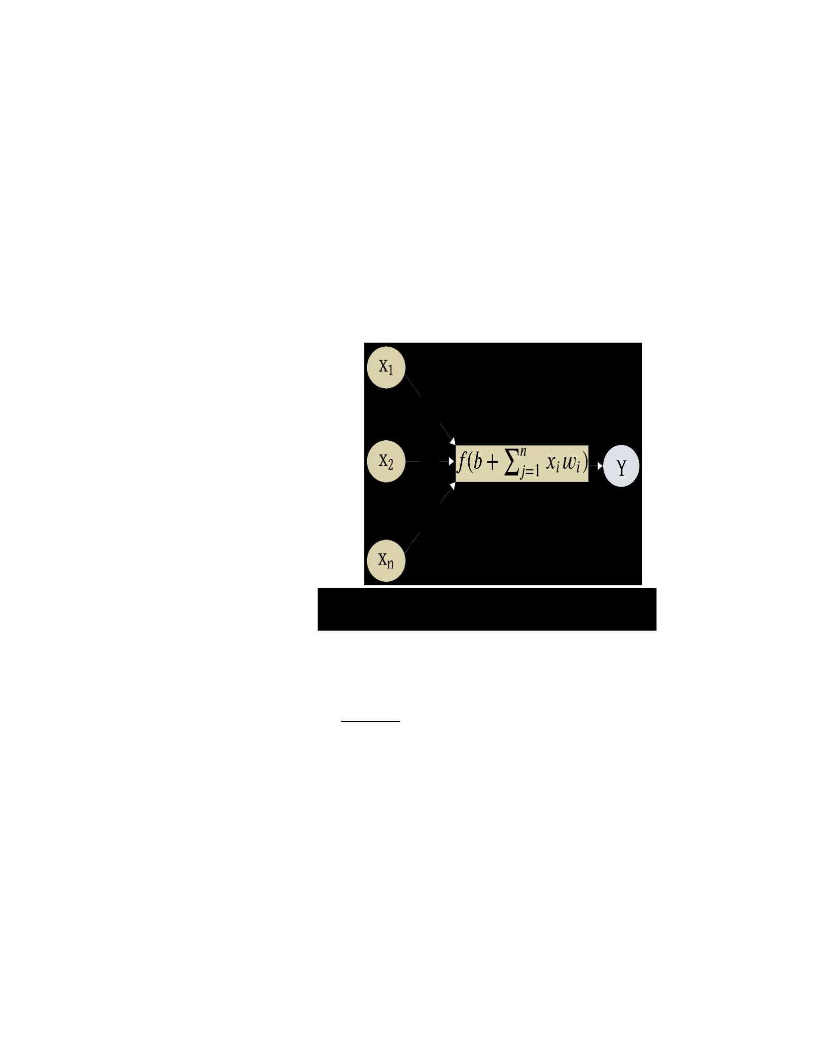
use of activation functions. The function is attached to each neuron in the network and
determines whether that neuron should be activated or not, based on the weighted sum of its
input (see Figure 2.10. ). During the training phase, activation functions introduce non-linearity
into the models, enabling them to learn and represent complex relationships. They also play a key
role in the backpropagation process, which is used to update the weights in the network. The
derivative of the activation function is used to calculate the gradient of the loss function with
respect to the weights, which is then used to update the weights in a direction that reduces the
overall loss. During the inference stage, when new data is presented to the model for prediction,
the activation functions are used in the forward pass of the model to generate the outputs of each
layer, ultimately leading to the model's final prediction.
There are several activation functions utilized in CNNs, each with their unique
characteristics and advantages. In this section, we briefly discuss some of the most used
activation functions, including the Rectified Linear Unit (ReLU) [74], Sigmoid [25], Hyperbolic
Tangent (tanh) [75], Softmax [32], and Leaky ReLU [71].
Rectified Linear Unit (ReLU)
ReLU [5] is one of the most widely used activation functions due to its simplicity and
efficiency. Mathematically, it is defined as:
𝑅𝑒𝐿𝑈(𝑥) = 𝑚𝑎𝑥(0, 𝑥)
(2. 10)
This function essentially keeps the positive inputs as is and sets all negative inputs to
zero. This simple function allows for fast computation while introducing non-linearity into the
model. However, one of the downsides of ReLU is that it can cause the dying ReLU problem
[76], where some neurons are never activated, causing their weights to remain unadjusted.
Sigmoid
The sigmoid function [77] transforms the input to a range between 0 and 1, making it
especially useful for binary
classification problems.
However, it suffers from the
vanishing gradient [75]
problem, where the gradients
become increasingly small as the
absolute value of the input
increases. Formally, sigmoid is
defined as:
1
𝑆𝑖𝑔𝑚𝑜𝑖𝑑(𝑥) = C
(2. 11)
Hyperbolic Tangent (tanh)
Figure 2.10. Visualizing The Transition in Activation
Function
�
�
1 + �
�
3
The tanh function [31] is like the sigmoid function but transforms the input to a range
between -1 and 1, providing a zero-centered output. Like sigmoid, it also suffers from the
vanishing gradient problem. Formally, tanh is defined as:
𝑒C− 𝑒3C
𝑡𝑎𝑛ℎ(𝑥) = 𝑒C + 𝑒3C .
(2. 12)
Leaky ReLU
Leaky ReLU [71] is a variant of ReLU designed to fix the dying ReLU problem. It allows
a small, non-zero gradient when the unit is not active. Mathematically, it is defined as:
𝐿𝑒𝑎𝑘𝑦𝑅𝑒𝐿𝑈(𝑥) =
𝑚𝑎𝑥(0.01𝑥, 𝑥)
(2. 13)
The parameter of 0.01 is adjustable and can be tuned for specific applications.
Softmax Function
Softmax function [29] is typically used in the output layer of a CNN for multi-class
classification problems. It converts the network's output into a probability distribution over the
target classes. The Softmax function is defined as:
𝑒C&
𝑆𝑜𝑓𝑡𝑚𝑎𝑥 ∑5 𝑒C’
(2. 14)
CNN Training and Optimization Algorithm

During training, CNNs aim to find the optimal parameters (filter weights and biases) 𝜃
that closely approximate the target mapping function 𝑓(𝑥;𝜃). In practice, 𝑓 fitted using
supervised or unsupervised training approaches [63].
Unsupervised learning [32] involves using unlabeled training data to learn the underlying
structure or distribution in the data. Here, unlabeled training data refers to a dataset in which
examples include the input data but not the corresponding target output. In unsupervised learning,
the model learns to identify patterns in the input data on its own and can be used to train CNNs
for tasks such as feature extraction or learning representations, where the goal is to identify
meaningful patterns or structures in the input images.
Supervised learning [32], on the other hand, involves using labeled training data to learn a
function that maps inputs to their corresponding outputs. In this context, labeled training data
refers to a dataset in which every example includes both the input data and its corresponding
target output.
Given that this dissertation focuses on image classification tasks, the training process
discussed herein will be in the context of supervised learning. In supervised learning, the training
data denoted as
𝐷 = {(𝑥%, 𝑦%): 1 ≤ 𝑛 ≤ 𝑁},
(2.
15)
comprises both the input values 𝑥% (e.g., an image) and corresponding desired output values 𝑦%
≈ 𝑔(𝑥%) (e.g., class label) [64]. N is the total number of samples in the training set. The training
process is broken down into two main steps: forward propagation and backpropagation (or
backprop) [63].
Forward Propagation
During forward propagation, the input data are passed through the network, layer by
layer, until they reach the output layer [8]. At each layer, the network applies a series of

transformations defined by the layer's weights, biases, and activation function [74]. The aim is to
generate a prediction 𝑦′% for each input 𝑥%. The forward propagation through a layer 𝑙 can be
represented by the function:
𝑓"(𝑥") = 𝜎(𝑊". 𝑥"
+ 𝑏"),
(2. 16)
where 𝑊" and 𝑏" are the weights and biases at layer 𝑙, 𝑥" is the output from the previous layer,
and 𝜎 is the activation functions [72].
With each iteration, the operation continues from the input layer to the output layer,
applying the transformations determined by each layer's parameters. For each input 𝑥%, the
output 𝑦′%represents the network's prediction for the corresponding target 𝑦%. The
discrepancy between the network's predictions and the actual targets, encapsulated in a loss
function 𝐿, forms the basis for the subsequent backpropagation process, which adjusts the
weights and biases in the network
to minimize the loss.
Backpropagation
After forward propagation, the network produces an output prediction 𝑦′%for each
input 𝑥% in the training set 𝐷. The network's goal is to make its predictions as close as possible
to the actual target values 𝑦%,as captured by the loss function 𝐿 [63]. Backpropagation is
the process used to adjust the network's parameters to minimize this loss [32].
Backpropagation starts by calculating the derivative of the loss function with respect to
the
network's output (also known as the output gradient). This derivative represents how much the
loss function will change if the network's output changes slightly. After that, for each layer in the
network, the derivative of the loss with respect to the layer’s parameters is calculated.

Mathematically, the backpropagation for given layer 𝑙 can be represented by the chain
rule
[78] as follows:
𝛿𝐿 𝛿𝐿 𝛿𝑓"
=∗ ,
(2. 17)
𝛿𝑊"𝛿𝑓"𝛿𝑊"
𝛿𝐿 𝛿𝐿 𝛿𝑓"
= ∗ ,
(2. 18)
𝛿𝑏"𝛿𝑓"𝛿𝑏"
where DE is the gradient of the loss with respect to the output of layer 𝑙, DF" and DF" are the
DF"D/"D/" gradients of the layer’s output with respect to its weights and biases
respectively.
Once the gradients are calculated, they are used to update the weights and biases in the
network [79]. The optimization process continues until the loss falls below a pre-specified
threshold or does not decrease significantly from one iteration to the next, indicating that the
network's parameters have converged to an optimal set [30]. The most common Optimization
Algorithms used in CNN for image classification tasks are discussed in the sections below.
Training Protocols
Parameter optimization during training can be executed under different protocols. The
two most common ones are stochastic training and batch training, each offering a distinct
approach towards learning the optimal weights [80].
Stochastic Training

In stochastic training [81] approach, an input sample 𝑥% is chosen at random for each
update of the network weights. This sample is used to compute error using a function 𝐸%(𝑤),
which quantifies the discrepancy between predicted output 𝑦′% and the actual target 𝑦% of the
𝑛 − 𝑡ℎ training sample.
𝐸%(𝑤) = 𝐿(𝑦G%, 𝑦%)
(2. 19)
The weights are then updated according to equations (16) and (17) with the derivatives computed
as 𝑊"%#H = 𝑊"I"J − 𝛼 . D KD(/(H" )
and 𝑏"%#H = 𝑏"I"J − 𝛼 . DKD(L("H) for weights and biases
respectively
[25].
Stochastic training has the advantage of being computationally efficient, as it requires
computing the gradients for only one example at a time [81]. However, because the updates are
based on single examples, they can be noisy and the convergence to the optimal set of parameters
can be slow [82].
Batch Training
Batch training , on the other hand, involves processing all 𝑁 inputs in the training set
before updating the weights [32]. The update is based on the overall error function 𝐸(𝑤), which
is the sum of the errors for all training examples:
M
𝐸(𝑤) = ‘ 𝐸%(𝑤).
(2. 20)
%64

Batch training can lead to more stable and reliable updates than stochastic training, but it
requires more computational resources, as it involves computing the gradients for all examples in
the training set at each step [82].
Mini Batch Training
In practice, a compromise between stochastic and batch training is often used. This
approach is known as mini-batch training. In mini-batch training, the training set is divided into
small batches of size |𝐵| [83]. Each update of the weights is based on the error function for batch
𝐵.
M
1
𝐸N(𝑤) = |𝐵| ‘ 𝐸%(𝑤).
(2. 21)
%64
Mini-batch training strikes a balance between the computational efficiency of stochastic
training and the stability of batch training [79]. It is currently the most used training protocol in
deep learning [32].
Loss Functions
Loss functions guide the optimization algorithm by providing a measure of the network's
performance. Here, we discuss loss functions commonly used in image classification tasks [32].
Mean Squared Error (MSE)
Also known as the Quadratic loss or L2 Loss, this function computes the mean of the
squared differences between the predicted 𝑦′% and actual output 𝑦% [33]. Although more
common in regression problems, it is occasionally used in binary and multi-class classification
tasks as well.
Mathematically, MSE is computed as follows:
M
1G.
(2. 22)
𝐸(𝑤) = 𝑁 ‘ 𝑦%− 𝑦 %
%64
where N is the total number of examples in the batch. The squaring operation ensures that each
term is positive and that larger deviations between 𝑦%and 𝑦′% contribute more to
the overall loss.
Cross-Entropy Loss
Also known as Log Loss, this function is frequently used in binary and multi-class
classification problems when the output is a probability distribution [84]. It measures the
dissimilarity between the predicted probability distribution 𝑦′% and the true distribution 𝒚𝒏. It's
preferred because it heavily penalizes confident yet incorrect predictions. Cross-Entropy loss can
be expressed mathematically as:
𝐸(𝑤) = − ‘ 𝑦% 𝑙𝑜𝑔 𝑦G% .
(2. 23)
%
In binary classification, 𝑦% and 𝑦′% represent the actual label and predicted probability
of the positive class for the 𝑛 − 𝑡ℎ example, respectively [32]. For multi-class classification, the
sums are over the classes.
Hinge Loss
The hinge loss, which originates from the realm of Support Vector Machines (SVMs)
[85], has also found applications in the context of neural networks, especially for binary
classification tasks. The underlying idea of hinge loss is the concept of "max-margin"
classification – it doesn't just aim to correctly classify training examples, but also seeks to

maximize the decision boundary (or margin) between classes [86]. This characteristic of hinge
loss often leads to better generalization on the test data. The hinge loss function for binary
classification can be mathematically represented as:
𝐸(𝑤) = ‘ 𝑚𝑎𝑥 (0, 1 − 𝑦%. 𝑦G%).
(2. 24)
%
The hinge loss function effectively ignores any data point that is classified correctly and
is outside the margin, focusing instead on misclassified points and those within the margin. This
property makes the hinge loss function particularly suited to handling outliers in the training data
and helps the trained model to generalize better to unseen data.
Sparse Categorical Cross entropy Loss
This variant of the standard Cross-Entropy loss is typically used in multi-class
classification tasks, particularly when the class labels are represented as integers rather than
onehot encoded vectors [87]. It's a useful option when dealing with a large number of classes as
it is more memory efficient. The mathematical formulation of this loss is as follows:
𝐸(𝑤) = − ‘ 𝑙𝑜𝑔 𝑦GO(.
(2. 25)
%
In this equation, 𝑦% is the integer class label for the 𝑛 − 𝑡ℎ example, and 𝑦′ is the
predicted probability distribution across classes for the 𝑛 − 𝑡ℎ example. Notably, 𝒚′𝒚𝒏 denotes
the predicted probability for the true class 𝑦%. The aim of the training process is to maximize
this predicted probability, effectively minimizing the negative log-likelihood.
When the model makes a correct prediction, i.e., the model assigns a high probability to
the correct class, the value of the negative log-likelihood is close to zero [32]. On the other hand,

if the model prediction is incorrect (with a low probability for the correct class), the loss becomes
significantly large. In this manner, Sparse Categorical Cross-entropy loss penalizes the model
proportionally to the disparity between the model's predictions and the actual class labels
[29].
Optimization Algorithms
The main purpose of optimization algorithms [72] is to iteratively tweak model
parameters to minimize the value of the loss function and improve the model's performance.
Since the advent of deep learning, several optimization algorithms have been developed. The
most used ones in CNNs are Stochastic Gradient Descent (SGD), RMSProp, Adam, and
AdaGrad.
Gradient Descent
Gradient Descent (GD) [72] is the most basic optimization algorithm not just in the field
of deep learning, but in all of machine learning. GD it iteratively adjusts model's parameters to
minimize a loss function. Mathematically, the update rule for a weight 𝑊 in GD can be
expressed as:
𝛿𝐸(𝑤)
𝑊" = 𝑊"− 𝛼 . 𝛿𝑊",
(2. 26)
and each bias 𝑏" is updated as:
𝛿𝐸(𝑤)
𝑏" = 𝑏"− 𝛼 . 𝛿𝑏",
(2. 27)
where 𝛼 a hyperparametric called learning rate that controls the size of the updates [88]. The

!𝑬 !𝑬 gradients and are computed using the chain rule equations 16 and
17 respectively.
!#!!$!
Stochastic Gradient Descent
While GD uses the entire training data to compute the gradient of the loss function,
stochastic gradient descent (SGD) [63] approximates the overall gradient using a single example
at each iteration. The central idea behind SGD is to adjust the model's parameters in the opposite
direction of the gradient of the loss function [30]. It calculates the derivative of the loss function
with respect to each parameter to decide the direction of the movement in the parameter space
[89]. Although SGD can be noisy due to the high variance in the updates, it often converges
much faster in practice because it processes fewer examples at a time [32].
Mini-Batch Gradient Descent
A compromise between GD and SGD, Mini-batch gradient descent (MB-GD) uses a
mini-batch of |𝐵| training examples at each step to compute the gradient [83]. This provides a
balance between the efficient computation of GD and the faster convergence of SGD. The update
rule in MB-GD is:
|N|
1 𝛿𝐸%& ,
(2. 28)
𝑊" = 𝑊"− 𝛼 . |𝐵| ‘964 𝛿𝑊"
where 𝐸%& is the error for the 𝑖 – 𝑡ℎ sample in the mini batch.
Adaptive Moment Estimation (ADAM)
Adam [79], short for Adaptive Moment Estimation, is a popular optimization algorithm
used in classification tasks. It's an optimization algorithm that combines the advantages of two
other extensions of stochastic gradient descent: AdaGrad and RMSProp [79].

Adam computes adaptive learning rates for different parameters. In addition to storing an
exponentially decaying average of past squared gradients like, Adam also keeps an exponentially
decaying average of past gradients. This combination allows the algorithm to not only scale the
learning rate like RMSProp, but also to benefit from the momentum by using the moving
averages of the gradients.
Adam's update rule involves:
𝑚
𝑊",
(2. 29) √𝑣 + 𝜀
where 𝑚 is an estimate of the first moment (the mean) of the gradients computed using:
𝛿𝐸
𝑚 = 𝛽4𝑚 + (1 − 𝛽4) 𝛿𝑊"
(2. 30)
and 𝑣 is an estimate of the second moment (the uncentered variance) of the gradients computed
by:
𝛿𝐸 R
𝑣 = 𝛽R𝑚 + (1 − 𝛽R) 𝛿𝑊"
(2. 31)
Here 𝛽4 and 𝛽R are the exponential decay rates for these moment estimates, and 𝜀 is a small
scalar to prevent division by zero [79].
Momentum
= 𝑊
"− 𝛼.

Another widely used technique during iterative optimization is momentum [82].
Momentum is a method that helps accelerate SGD in the relevant direction and dampens
oscillations [82]. It does this by adding a fraction 𝛾 of the update vector of the past time-step to
the current update vector. While momentum is not an optimization algorithm on its own, it plays
a crucial role in enhancing the performance of these algorithms. The update rule for SGD with
momentum is:
𝛿𝐸
𝑣 = 𝛾𝑣 − 𝛼
(2. 32) 𝛿𝑊"
𝑊"= 𝑊"+ 𝑣
(2. 33)
where 𝑣 is the velocity (the direction and speed of the gradient) and 𝛾 is the momentum term.
Momentum helps the optimization algorithm navigate along the relevant directions and
softens the oscillations in the irrelevant directions [82]. This becomes significantly important in
deep learning where we usually deal with high dimensional data and the optimization landscape
fraught with saddle points and local minima [30].
Regularization Techniques
Regularization techniques are crucial in training convolutional neural networks as they
help prevent overfitting, which occurs when the model performs exceedingly well on the training
data but poorly on unseen data [63]. Overfitting happens when the model learns to fit not only
the underlying pattern but also the noise in the training data, making it perform poorly on new
inputs [29]. This section will outline some of the most common regularization techniques used in

CNNs.
Weight Decay (L1 and L2 Regularization)
Weight decay is a common regularization method that discourages learning a more
complex or flexible model, to avoid the risk of overfitting. It does this by adding a L1 or L2 cost
associated with having large weights to the loss function [90]. L1 regularization adds an L1
penalty equal to the absolute value of the magnitude of coefficients [91]. In other words, it
subtracts a factor proportional to the absolute value of the weights from the weight vector at each
training step. L2 regularization adds a penalty equal to the square of the magnitude of
coefficients. This results in the weights vector being scaled by a factor just less than 1 [92].
𝐿4 = ‘ |𝑊9|
(2. 34)
9
𝐿R = ‘ 𝑊9R
(2. 35) 9
Dropout
Dropout is a technique used to combat overfitting where randomly selected neurons are
dropped during training [73]. The dropped neurons contribution to the activation of downstream
neurons is temporally removed on the forward pass and no weight updates are applied to the
neuron on the backward pass. It forces the network to learn more robust features that are useful
in conjunction with many different random subsets of the other neurons. This ensures that no
single neuron becomes overly specialized or overly reliant on the output from another specific

neuron. This can help the network be more robust as it is forced to learn redundant
representations for features. If one path which recognizes a feature fails, another might succeed
[73].
Batch Normalization
Batch normalization [93] is a technique designed to automatically scale the inputs to a
layer. When applied to a layer of a CNN, it has the effect of dramatically accelerating the training
process and providing a form of regularization, often eliminating the need for Dropout
[94].
Data Augmentation
Data augmentation encompasses a wide range of techniques used to generate “new”
training samples from the original ones by applying random jitters and perturbations (such as
random rotations, shifts, flips, etc.) [95]. But the main idea remains the same: the model can
learn more robust features by seeing more variations of the data.
Early Stopping
In this form of regularization, we stop the training process before the model starts to
overfit. This is typically achieved by splitting the training data into a training set and a validation
set. The model is trained on the training set, and the model's performance is evaluated against the
validation set after each epoch. Training is stopped as soon as the performance on the validation
set starts to degrade (i.e., the loss starts to increase, or the accuracy starts to decrease) [96].
Essential Terminologies in Deep Learning
A clear understanding of the terminologies used in this research domain, such as
parameters, hyperparameters, epochs, and iterations, is crucial. These terms are often used
interchangeably, but they refer to different concepts that play a significant role in the design,
training, and performance of CNNs.

Parameters vs Hyperparameters
In machine learning, and particularly in ANNs, a distinction is often made between
parameters and hyperparameters [97]. Parameters refer to the variables that the model learns
through training. In the case of a neural network, these would be the weights (𝑊) and biases
(𝑏) (Equation 2.9) that are adjusted through the backward propagation process during training
[63].
Hyperparameters, on the other hand, are variables that are set before the model training
process begins. These cannot be learned from the training process and must be provided by the
user. In a neural network, hyperparameters include the learning rate (α), the activation function
selection, the number of iterations, the kernel size for convolutional layers, and the number of
hidden layers and nodes in each layer. The tuning of hyperparameters can significantly affect the
performance of the model, and hence, an appropriate selection of hyperparameters is a critical
part of training a neural network [63].
Epochs vs Iterations
Another set of terms that often get conflated are epochs and iterations, but they refer to
different aspects of the training process. Iteration refers to the number of batches needed to
complete one epoch. It is defined as the process of passing one batch of input data through the
network (in both forward and backward direction) once.
Epoch, on the other hand, refers to passing the entire training dataset through the network
once (which would include many iterations). For example, if you have 1280 training examples
and you choose a batch size of 64, then an epoch will consist of 20 iterations.
The number of epochs is also a hyperparameter that can be adjusted. Setting this number
too high might lead to overfitting, as the network might start to learn noise and details from the
training set that don't generalize well to unseen data. Conversely, setting the number of epochs
too low might mean that the network has not learned the relevant patterns in the training data,
leading to underfitting.

Transfer Learning and Fine Tuning
The concept of transfer learning is a breakthrough in the field of deep learning [98] ,
[51]. This approach allows us to leverage the knowledge acquired from previous models and
apply it to new, similar tasks, resulting in models that require significantly less data, compute
time, and overall training effort [63]. CNN architectures, which have achieved state-of-the-art
results in tasks such as image classification on the ImageNet dataset [99] or object detection on
the COCO dataset [100], are often the source of this pre-learned knowledge. However, the
classifiers in these models are typically fine-tuned to specific applications. To repurpose these
architectures for different tasks, it is necessary to adjust the classifier to fit the requirements of
the new application [101].
After such modifications, there are typically three strategies available for training the new
model.
Training from Scratch
This approach involves initializing a new model and training it using the new dataset.
This method requires the most resources and time and is typically used when there is a
significant amount of labeled data available for the new task [63].
Freezing and Fine–Tuning
This approach involves freezing the weights of some layers (usually the early
convolutional layers) and training the remaining layers on the new dataset [32]. This is typically
done when the new task is similar to the original task the pre-trained model was trained on, and
there is not a lot of data available for the new task.
Fine-Tuning from a Pre-trained Model
This approach involves initializing the model with weights from a pre-trained model and
then continuing to train the model on the new dataset [63]. This is typically done when the new
task is similar to the original task the pre-trained model was trained on, and there is a moderate
amount of data available for the new task.

In this research, to understand the effect of our proposed strategies, we have adopted the
approach of training from scratch.
Training vs Test Sets in Deep Learning
Since the objective of building models is to make accurate predictions on new, unseen
data, the dataset is usually divided into primarily two sets - a Training set and a Test set.
Training Set
The training set is the portion of the data set that we use to train our model. It includes
both input data and the corresponding correct output. The proportion of the total dataset used for
training typically ranges from 60% to 80% [32]. A common practice is to further divide this set
into two parts: a slightly smaller training set, and a validation set. The model is trained on the
training set and the performance of the model (loss, accuracy, etc.) is evaluated on the validation
set after each epoch – commonly referred to as cross-validation. This helps monitor the model's
learning progress and also detect if the model is starting to overfit the training data. The model's
hyperparameters (like learning rate, number of epochs, batch size, etc.) are adjusted based on the
performance on the validation set.
Test Set
The test set is the portion of the dataset that the model has not seen during its training
phase [32]. It is used to test the performance of the model on unseen data, and assess its ability to
generalize to new, unseen scenarios. The proportion of the total dataset used for testing typically
ranges from 20% to 40%. This final evaluation on this set provides us with an unbiased estimate
of the model's performance on an unseen dataset and gives us an indication of how well the
model will perform when deployed in the real world.
In deep learning, the size of the dataset and the complexity of the model architecture can
play a significant role in how the data is split and used. However, the underlying principle
remains the same - learn from the training data, validate and tune using the validation data, and

finally test on the test data. This rigorous process helps ensure that the model is well-trained,
tuned, and ready to tackle real-world data [63].
Analysis and Metrics
An important aspect of evaluating a model's performance is understanding how well it
generalizes - that is, how effectively it handles data that it hasn't seen during training [102]. Since
the goal is to build a model that predicts accurately on unseen data, the test set, which is held-out
during training, is used to assess the generalization power of the model. Various metrics are
utilized to quantify this performance, which are calculated based on the model's predictions on
this test set and their comparison with the true labels.
Accuracy
This is the most straightforward metric. It measures the proportion of correctly classified
instances out of the total instances [103]. If we denote the number of correctly classified
instances as True Positives (𝑇𝑃) and True Negatives (𝑇𝑁), and the incorrectly classified
instances as False Positives (𝐹𝑃) and False Negatives (𝐹𝑁), then accuracy can be formulated
as:
𝑇𝑃 +𝑇𝑁
𝐴𝑐𝑐𝑢𝑟𝑎𝑐𝑦 =
(2. 36)
𝑇𝑃 +𝑇𝑁 +𝐹𝑃 +𝐹𝑁
Precision
Precision, also called Positive Predictive Value (PPV), is the ratio of correctly predicted
positive observations to the total predicted positives. Precision is a measure of a classifier's
exactness. A low precision indicates a high number of false positives.
𝑇𝑃
𝑃𝑟𝑒𝑐𝑖𝑠𝑖𝑜𝑛 =

(2. 37) 𝑇𝑃 + 𝐹𝑃
Recall (Sensitivity)
Recall, also called True Positive Rate (TPR) or Sensitivity, is the ratio of correctly
predicted positive observations to all observations in actual class. Recall is a measure of a
classifier's completeness. A low recall indicates a high number of false negatives.
𝑇𝑃
𝑅𝑒𝑐𝑎𝑙𝑙 =
(2. 38) 𝑇𝑃 + 𝐹𝑁
F1 Score
The 𝐹1 Score is the weighted average (harmonic mean) of Precision and Recall.
Therefore, this score takes both false positives and false negatives into account [104]. It is
suitable for uneven class distribution problems.
𝐹
(2. 39)
𝑃𝑟𝑒𝑐𝑖𝑠𝑖𝑜𝑛+𝑅𝑒𝑐𝑎𝑙𝑙
Receiver Operator Characteristic (ROC) Curve
ROC [105] is another effective method commonly used for assessing the performance of
a diagnostic test tools for medical applications. ROC considers the true positive, true negative,
false positive and false negative predictions of the model. It is a plot that depicts the trade-off
between sensitivity and 1-specificity where sensitivity is the fraction of positive patterns that are

correctly classified, and specificity is the fraction of negative patterns that are correctly
classified. The area under a ROC curve (AUC) is the single and most used index for measuring
the performance of a test. Unlike the threshold metrics above, the AUC value reflects the overall
prediction performance of a classifier. The closer the AUC value is to 1 the better the
performance of the models is on real-world data.
Summary
In this chapter, we offered a comprehensive overview of the fundamental concepts and
theoretical underpinnings that form the basis of this research. It began with a broad introduction
to the field of deep learning and artificial neural networks (ANNs), highlighting their pervasive
influence on various scientific and commercial applications. We had dived into the inner
workings of ANNs, specifically focusing on Convolutional Neural Networks (CNNs), given their
prevalent use in image classification tasks.
In addition, this chapter provided a strong foundation in CNNs, covering their structure,
operation, training mechanisms, and evaluation metrics. It laid the groundwork necessary to
understand the methodologies and techniques that will be employed in the following chapters of
this dissertation. As we move forward, we will apply these principles in practice and evaluate
their performance in the context of our specific research objectives.

CHAPTER 3
LITERATURE REVIEW
Introduction
Numerous theories and methodologies have emerged, each contributing unique
perspectives and advancing our understanding of deep learning. This chapter presents relevant
literature, focusing on several areas that have inspired the direction of this dissertation.
Firstly, we explore some intriguing properties of neural networks [15], which, despite
their seemingly simple structure, exhibit a multitude of complex behaviors. From their ability to
approximate any function (universal approximator) to their ability to learn from noise-only data
[18], these properties provide a fundamental understanding of the capabilities and limitations of
neural networks.
We then transition into an information theoretic interpretation of deep learning [106]. By
applying concepts from information theory, we gain a fresh perspective on how neural networks
learn and generalize. This understanding allows us to better comprehend the interplay between
model complexity, data complexity, and training dynamics which in turn motivates us to utilize
the field of information theory to devise techniques that enhance deep learning.
An analogous approach is taken towards understanding images. Through an
informationtheoretic lens, we explore how image data's inherent structure and complexity
influence CNNs' learning and performance.
Lastly, we delve into the concept of curriculum learning, an approach that leverages the
principle of learning from easy to hard examples. This approach has demonstrated promising

results in enhancing model performance and expediting the learning process, suggesting exciting
potential for future developments in CNN training.
In each section, we not only summarize the key findings but also highlight their
implications for our research, providing a solid theoretical foundation for the subsequent
experimental work. Through this exploration, we hope to contextualize our research within the
broader landscape of the field and highlight the novel contributions that our work aims to
provide.
Intriguing Properties of Neural Networks
Neural networks, specifically Convolutional Neural Networks (CNNs), have an
impressive ability to learn from variety of datasets, but does this capacity extend to those
containing samples uncorrelated with their labels? Can they derive meaning from a dataset
consisting only of noise? In essence, can these networks discern patterns where our human eyes
see none? Zhang et al. (2016) and Szegedy et al. ( 2013) set out to explore these questions, and
their findings are nothing short of intriguing. They demonstrated that CNNs can comfortably fit a
training set composed of samples that have no correlation with labels (refer to Figure 10 (right)
for an illustrative example).
The high expressivity of CNNs, while a significant factor in their success across various
tasks, also leads them to learn uninterpretable representations with somewhat counterintuitive
properties. This unexpected behavior might be attributable to the well-established fact that most
multi-layer, feed-forward networks act as universal approximators. Hornik et al. demonstrated
that these feedforward networks, which form the basis of many modern CNN architectures, can
approximate any Borel measurable function, from one finite-dimensional space to another, with
remarkable accuracy.
In simpler terms, CNNs are equipped to learn representations from any data, regardless
of whether these representations hold characteristics that researchers can identify or even make
sense of. The universality of CNNs has been confirmed, either directly or indirectly, by several

researchers [18]. This property provides a glimpse into the immense potential of these networks
and raises exciting questions about their capabilities, some of which we will continue to explore
in this chapter.
Building upon the intriguing properties of neural networks, Szegedy et al. [15] uncovered
an unexpected level of discontinuity in the input-output mapping learned by deep networks. They
demonstrated that the application of a certain almost imperceptible perturbation to an input
image could cause the network to misclassify it completely. This peculiarity, known as the
adversarial examples, illustrates the surprising fragility and lack of robustness in the models
which perform impressively well on their training data.
Such findings challenge the conventional perspective that neural networks construct a
hierarchy of features with increasing levels of abstraction. According to this traditional view, the
networks learn to combine pixels to form edges in the lower layers, then learn to assemble these
edges into parts of objects in the middle layers, and so on. This hierarchical structure, intuitive
and appealing as it may be, might not hold true given the aforementioned properties of neural
networks. The ability of networks to learn from uncorrelated samples and their sensitivity to
minuscule input changes suggest a learning process that is far more complex and less
interpretable than a simple building-up of abstract features.
It is these key findings that form the foundation for this these. They urge us to reassess
our understanding of what neural networks truly learn and how they arrive at their impressively
accurate predictions. The journey to unveil these mysteries necessitates a deep dive into the
theory underlying neural networks, a task we undertake in the next section.
Information Theory Interpretation of Deep Learning
Information theory, which was introduced by Claude Shannon in the 1940s [107],
provides a mathematical framework for understanding and quantifying the concept of
information. It introduces core concepts like entropy, which measures the uncertainty or

randomness in a set of data, and mutual information, which quantifies the amount of information
that can be obtained about one random variable by observing another.
An interpretation of Deep Learning through the lens of Information Theory provides a
mathematical model that could shed light on the otherwise "black box" nature of Deep Learning
models. This interpretation is primarily based on the Information Bottleneck (IB) [108] principle.
The Information Bottleneck Principle
In the context of deep learning, the Information Bottleneck (IB) principle offers an
illuminating perspective. The IB method, introduced by Tishby et al. [108], provides a formal,
information-theoretic framework for understanding the trade-off between the complexity and
accuracy of a representation. It is an approach to summarize data in the most compact
representation that retains the most about the variables we are interested in. Formally, the
Information Bottleneck method is an optimization problem defined by:
𝑎𝑟𝑔𝑚𝑖𝑛 𝐼(𝑋;𝑇) −
𝛽𝐼(𝑇; 𝑌),
(3. 1)
S(T|U)
where:
•𝑋 is the original input variable.
•𝑇 is the compact representation of the variable.
•𝑌 is the variable we are interested in.
•𝐼(𝑋; 𝑇) is the mutual information between the input and its representation.
•𝐼(𝑇; 𝑌) is the mutual information between the representation and the output.
•𝛽 is a trade-off parameter between the complexity of the representation and the retained
information about the output.

A solution to this problem determines the representation 𝑇 that extracts the relevant
information from 𝑋 about 𝑌 as efficiently as possible.
Application to Deep Learning
In the context of Deep Learning, each layer of an ANN can be seen as learning a
representation (or summary) of the data. The learning process aims to find a representation that
retains as much information about the target output as possible while being as compact as
possible.
Saxe et al. [106] propose to model this learning process as solving a sequence of IB
problems, one for each layer of the network. In this model, each layer is seen as a set of summary
statistics about the data and labels. The measure of these statistics (the amount of information
each layer retains about the data and labels) changes over the course of training.
By using this interpretation, we can use Information Theory measures to quantify how
much information is retained or lost at each layer, thus providing a quantitative way to
understand and analyze the learning process.
Information Theoretic Measures for Image Characteristics
Applying information theory to image characteristics can help us better understand the
image content. For instance, we can use entropy to evaluate the 'complexity' of an image region.
A high entropy region might indicate a complex texture, possibly requiring a more complex
model for accurate classification.
By extending such measures to assess the relationships between training samples, we can
develop a statistical understanding of our data that can guide our machine learning models. For
example, by understanding the mutual information between different classes of images, we can
inform our model about which classes are easier to distinguish, and which ones might be harder.
These information theoretic approaches not only provide a rigorous way to analyze image
data, but they can also influence how we preprocess images and design our machine learning
algorithms. In the following section, we will discuss how these principles tie into curriculum

learning - an approach to learning optimization that organizes the presentation of training
samples in a meaningful way to improve the learning process.
Relationship to Our Research
The IB principle and the extension of information theory to images are two powerful
concepts we use extensively. These tools allow us to quantify and study sample relationships
within datasets mathematically. By understanding how networks learn, gauging the amount of
information retained or lost at each layer, and identifying the factors influencing these processes,
we can foster more efficient and effective network designs, learning algorithms, and optimization
techniques.
We posit that if we preprocess our training data in a manner that efficiently captures
relevant information in the early stages of training, we can enhance the effectiveness and
efficiency of learning. To achieve this, we propose extending information theoretic techniques to
investigate image characteristics and the relationships between training samples. The goal is to
devise more effective learning algorithms.
Curriculum Learning
CL offers immense potential for advancing the field of deep learning. CL proposes an
orderly, sequential approach to training deep learning models, quite akin to how academic
curricula are structured. As humans, we learn new concepts gradually, progressing from simpler
to more complex tasks, while leveraging previously learned knowledge to assimilate new
information more effectively. Similar principles are at the heart of CL.
In the context of machine learning, CL was initially formalized by Bengio et. al. [19] and
has in recent years, gained some traction as a potential technique to further improve deep
learning [[19] [109] [110] [111] [22]]. At its core, CL seeks to answer a pertinent question - how
do we determine the best order of samples for training a model efficiently and effectively? In
machine learning, CL attempts to find some optimal sequence of training input (or training tasks

for transfer learning [111]) to optimize the learning process compared to no-curriculum (No-CL)
training.
Practically implementing CL, however, poses a few challenges. How do we ascertain the
'difficulty' of a training sample or task? How can we validate if the sequence indeed leads to
more efficient learning? These are the two challenges this dissertation sheds light on. We
leverage information theory and statistics to tackle these questions and develop a more
systematic approach to CL.
Summary
This chapter lays the foundation for the subsequent phases of this research, establishing a
solid theoretical background, drawing from two pertinent studies that form a foundation for our
research. The chapter begins by exploring the intriguing properties of CNNs, including their
universal approximation capabilities and their unexpected behavior when dealing with datasets
lacking correlation between samples and labels.
The discussion then shifts towards the Information Theory Interpretation of Deep
Learning. Using the Information Bottleneck (IB) principle, we provide a mathematical model
that sheds light on the learning process of these networks. Finally, we delve into the concept of
Curriculum Learning, an optimization technique influenced by human learning. By leveraging
information theory and statistics, we proposed solutions to the challenges inherent in
implementing Curriculum Learning, leading to the development of a systematic approach that
enhances deep learning algorithms.

CHAPTER 4
FRAMEWORK DEVELOPMENT AND IMPLEMENTATION
Introduction
This chapter details the implementation of Deep-CLO. The framework is grounded on an
information-theoretic perspective of digital images. This perspective facilitates the quantification
of training samples’ inherent characteristics, enabling us to develop an objective and measurable
understanding of samples and their interrelationships within the dataset. This quantitative
approach allows for a more precise formulation of curriculum learning schemes, tailored
preprocessing algorithms, and enhanced model training strategies. Deep-CLO achieves this
through three core modules:
•CLO – The core component, an end-to-end curriculum training mechanism that
synergizes a batch-based syllabus (ordering of samples by a certain measure) with
conventional backpropagation algorithms for deep neural network training.
•PROSIS-2D – A unique image preprocessing algorithm that proposes, analyzes, and
reconstructs by reorganizing image regions (patches) to yield enriched training samples.
This module addresses questions related to feature locality and its significance in image
learnability and classification.

•Volumizer Algorithm (PROSIS-3D) – A preprocessing technique that reconstructs 2D
training images as 3D volumes to allow for enhanced feature extraction and an effective
countermeasure against localized adversarial attacks.
These modules can be used individually or together to address some of the primary
questions guiding this research. They allow us to explore how human recognizable features in the
training set influence the learnability of a task, and if feature locality plays a significant role.
We use the framework to preprocess benchmark datasets such as CIFAR10 & 100 training and
train convolution-heavy past and more recent state-of-the-art (SOTA) CNN models.
Importantly, the Information Bottleneck (IB) principle forms the backbone of this
approach. The principle suggests that model training is essentially an act of information
extraction from the training data. This perspective aligns with our view that deep learning
models, through training, navigate the complex, high-dimensional data manifolds to find local
minima that represent useful feature representations. Thus, curriculum learning, and the
assessment of training samples' difficulty and characterizing datasets are essential in guiding
models to efficiently find a local minimum within the data manifolds.
The following section delves deeper into this information-theoretic perspective of images,
providing further details on how these principles are utilized to create a more effective and robust
deep learning framework.
Framework Implementation
In conventional training, where random shuffling is employed, determining the specific
aspects of training data that a model responds to at any given stage of learning or inference is still
challenging [112]. This black-box nature of deep learning limits our ability to interpret the
models, thereby constraining opportunities for further research, diagnostics, and innovation. We
believe it is crucial to understand the complex interplay between various factors and features that
influence a model's decision-making process for validating predictions, ensuring robustness, and
facilitating model adaptation to new domains or applications.

Our framework offers an innovative departure from traditional approaches, emphasizing a
structured sequence of inputs that is grounded in the intrinsic characteristics of samples, which
are quantified using objective metrics. This enhanced structure doesn't only bring organization
but, crucially, introduces traceability to the training process. This traceability – ability to track
and understand the sequence and reasoning behind how the model learns – facilitates an indepth
exploration of the model's learning trajectory, shining a light on the rationale behind how models
extract features.
This approach underlines the importance of focusing on the data manifold, investigating
how the inherent structure and characteristics of the data can be leveraged to facilitate efficient
learning. This is achieved through the application of assessment metrics in several ways:
•Sample Similarity: The framework employs these metrics to gauge the degree of
similarity between various samples within the training dataset. Understanding these
relationships helps inform the ordering of samples throughout the training process. An
approach in which we initiate the training process with a set of highly similar samples
adheres to the foundational principle of curriculum learning - transitioning from less
complex to more intricate tasks progressively.
•Uncertainty Reduction: Measures such as joint entropy act as an effective representation
of the combined uncertainty of two samples. Formulating a curriculum that incrementally
introduces samples with elevated levels of joint entropy can assist in managing the
model's uncertainty. This approach fosters a more structured and stable learning
progression, as it gradually exposes the model to higher degrees of complexity.
•Balancing Diversity and Redundancy: The framework harnesses these metrics to strike a
balance between diversity and redundancy in the learning process. For instance, samples
demonstrating lower levels of mutual information may contain overlapping or redundant
information, while those with higher joint entropy may offer diverse yet interconnected

concepts. Employing a learning strategy that navigates this balance can boost learning
efficiency.
Objective Assessment of Sample Complexity
Traditional approaches to curriculum learning often rely on intuitive or ad hoc methods to
determine the complexity of training samples. These methods can include focusing on superficial
traits of the data or initially training the model to understand sample difficulty based on the
incurred loss. However, these approaches can lead to challenges.
Surface-level traits of images, such as the number of objects present or the presence of
occlusion, may not accurately capture the underlying complexity inherent in the data, potentially
leading to an inefficient or misguided curriculum. Furthermore, using model loss as an indicator
of sample complexity assumes that the current state of the model provides an accurate estimate of
the inherent difficulty of a sample. This assumption may be misleading as deep learning models
are universal function approximators - their performance on a given sample at an arbitrary point
during training may not necessarily reflect the sample's true complexity.
Our framework offers a solution to these challenges by leveraging both information
theory and statistical measures. It provides an objective, mathematical means of quantifying the
inherent complexity and similarity within and among samples. This approach is independent of
the model's state and is purely based on the informational and statistical content of the data. It
allows us to capture more abstract representations of complexity that a deep learning model
grapples with during its training process.
In the following subsections we discuss both the information-theoretic perspective of
digital images, and the statistical methods used to assess and rank sample complexity.
Information-Theoretic Perspective of Digital Images and Assessment Metrics
At the heart of Deep-CLO lies a unique perspective: treating digital images as
twodimensional random variables, each pixel considered as an independent and identically
distributed (i.i.d) realization [113]. This perspective, which emerges from the field of

information theory, provides a mathematical framework for quantifying the amount of
information carried by a given data source [113]. When applied to digital images, this viewpoint
allows us to measure the inherent characteristics of a training set, individual samples, and their
interrelations within the dataset.
Information theory provides a theoretical foundation to quantify information
content, or the uncertainty, of a random variable represented as a distribution [113], [114].
Information theoretic measures of content can be extended to image processing and computer
vision [115]. One such measure is entropy. Intuitively, entropy measures how much relevant
information is contained within an image when representing it as a discrete information source
that is random [113]. Formally, let 𝑥 be a discrete random variable with alphabet 𝜒 and a
probability distribution function 𝑝(𝑥), 𝑥 ∈ 𝜒. The Shannon entropy [107] of 𝜒 is
defined as
1
𝐻(𝑋) = ‘ 𝑝(𝑥) 𝑙𝑜𝑔
(4. 1)
𝑝(𝑥)
C∈V
where 0𝑙𝑜𝑔 ∞ = 0 and the base of the logarithm determines the unit, e.g. if base 2, the
measure is in bits [116]. The term −𝑙𝑜𝑔 𝑝(𝑥) can be viewed as the amount of information
gained by
observing the outcome 𝑝(𝑥).
Entropy is usually meant to measure the uncertainty of a continuous random variable.
However, when applied to discrete images, it measures how much relevant information (in
contrast to noise) is contained within an image when representing the image as a discrete
information source [113]. Here, we construct probability distribution associated with each image
by binning the pixel values into histograms. The normalized histogram can then be used as an
estimate of the underlying probability of pixel intensities, i.e., 𝑝(𝑖) = $"((&), where 𝑏C(𝑖)
denotes the histogram entry of intensity value 𝑖 in 𝑥, and 𝑁 is the total number of pixels of 𝑥.
With this representation the entropy of an image 𝑥 can be computed as:
𝑁
𝐻(𝑥) = ‘ 𝑏C(𝑖) 𝑙𝑜𝑔 𝑏C(𝑖),
(4. 2)
where 𝐷is the training set and 𝜒 represents the image as a vector of pixel values.
Entropy provides a measure of the standalone complexity of a sample. Higher entropy
indicates a more complex image with more diverse features. This helps in sorting and sequencing
the samples from less complex (lower entropy) to more complex (higher entropy) during the
training, adhering to the principle of curriculum learning. See Figure 4.1 for illustration.
To fully understand the interactions and relationships between samples within our dataset,
we apply additional information-theoretic metrics that relate training samples to each other.
These include Joint Entropy, Kullback-Leibler Divergence, Mutual Information,
Information Variation, and Conditional Entropy. Each of these measures offers unique insights
into the interplay between samples within our training set. A summary of metrics is provided in
Table 1. For an even more comprehensive understanding of these metrics, we recommend
consulting references [74], [75], and [78].
Joint Entropy
Joint entropy (JE) allows us to measure the total uncertainty or information content in two
or more random variables, providing a way to quantify the combined complexity of multiple data
sources. By considering two images (or random variables) 𝑋 and 𝑌 as a single vector-valued
random variable, we can define their joint entropy JE(X, Y) with a joint distribution 𝑝(𝑥, 𝑦) as
follows:
𝐽𝐸 ‘ ‘ 𝑝(𝑥, 𝑦) 𝑙𝑜𝑔 𝑝(𝑥, 𝑦).
(4. 3)
C∈U O∈W
This equation sums the product of the joint probability and the log of the joint probability
across all possible combinations of 𝑥and 𝑦. The resultant value gives a measure of the
combined information in 𝑋 and 𝑌. It tells us how much information (on average) we would
expect to need to specify both the outcome of 𝑋 and 𝑌.
When it comes to images, joint entropy is usually computed by forming a joint histogram
between the two images. For two samples, 𝑥4, 𝑥R∈ 𝑇 the joint entropy is calculated by by:
𝐽𝐸(𝑥4, 𝑥R) = ‘ 𝑏C(𝑖) 𝑙𝑜𝑔 𝑏C(𝑖),
(4. 4)
9
where 𝑏C(𝑖) is the 𝑖&: value in the joint histogram. The joint histogram is constructed by
calculating the number of occurrences of each pair of intensity values (𝑖, 𝑗) in the same spatial
location of two images.
JE is useful in tasks that involve comparing the similarity or dependency between two
images, such as image registration. The smaller the joint entropy, the higher the dependency
between the two images (Figure 4.2). In our study, it provides a mechanism to assess the
dependency between training samples, which could help us better understand the structure and
relationships within the dataset and enhance the curriculum learning strategy.
measure used for quantifying the difference or 'divergence' between two probability distributions.
Formally, for two discrete probability distributions 𝑃 and 𝑄 defined on the same probability
space, the K-L Divergence of P from Q is given by:
𝑃(𝑥)
𝐷’E(𝑃 || 𝑄) = ‘ 𝑃(𝑥) 𝑙𝑜𝑔 𝑄(𝑥) ,

(4. 5)
9
This measure is not symmetric, meaning the K-L Divergence of 𝑄 from 𝑃 is not the
same as the K-L Divergence of 𝑃 from 𝑄. The value of the K-L Divergence is always non-
negative, and it becomes zero if and only if 𝑃 and 𝑄 are the same distribution.
When applying it to digital images, we treat the images as two-dimensional random
variables P and Q with the histogram of pixel intensities 𝑥4 and 𝑥R serving as an estimate of the
underlying probability distribution. Assuming the two images are 𝑥4 and 𝑥R, KL is defined as:
𝑥49 ,
(4. 6)
𝐷’E(𝑥4|| 𝑥R) = ‘9𝑥49 𝑙𝑜𝑔 𝑥R9
where 𝑖 the index of a pixel value taken from the distribution. This quantifies the amount of
information loss when one image is used to approximate another. It allows us to quantitatively
assess the 'similarity' or 'difference' between samples in our training set. By using this measure,
we organize samples from simpler to more complex, based on the divergence between their pixel
intensity distributions, contributing to an effective, information-theoretically grounded
progression for curriculum learning (see Figure 4.3).
Mutual Information
Mutual Information (MI) represents the amount of information that knowing one random
variable gives about another. It is the measure of the statistical dependency between two or more
random variables [16]. The mutual information of samples 𝑥 𝐷 is defined as a sum of the
individual entropies subtracted by the joint entropy of the two samples 𝐽𝐸(𝑥4, 𝑥R).

𝑀𝐼(𝑥4, 𝑥R) = 𝐻(𝑥4) + 𝐻(𝑥R) − 𝐽𝐸(𝑥4, 𝑥R)
(4. 7)
In essence, mutual information measures the reduction in uncertainty for one image given
the knowledge of another. As the mutual information increases, the statistical dependence
between the two images becomes stronger, indicating a higher level of similarity.
Maximizing mutual information has been found to be an effective technique in various
applications, as noted by [118]. It tries to find regions of complexity that overlap between two
images by maximizing the individual entropies, while simultaneously minimizing the joint
entropy, implying that the images explain each other well. As image similarity measure, mutual
information has been found to be successful in many application domains [118].
In the context of CL, mutual information is used to understand the dependency between
samples in the training set and help order them in a meaningful way (Figure 4.4). High mutual
information between samples might suggest a strong relationship, meaning that learning from
one sample could potentially enhance the learning from the other. Hence, ordering samples in
such a way that we progress from samples with less mutual information to those with more could
potentially aid in efficient learning.
Information Variation
Information Variation (IV) [114] offers a perspective into the differences and variations in
the information content between two random variables. Rather than measuring combined
complexity as Joint Entropy does, IV measures the variability or divergence between two data
sources.
Given two random variables 𝑋 and 𝑌, their individual entropies H(X) and H(Y) and
their mutual information MI(X; Y), we can compute their Information Variation 𝐼𝑉(𝑋, 𝑌) with
a joint
distribution 𝑝(𝑥, 𝑦) as follows:

𝐼𝑉(𝑋, 𝑌) = 𝐻(𝑋) + 𝐻(𝑌)
− 2 × 𝑀𝐼(𝑋; 𝑌)
(4. 8)
This equation determines the divergence between the marginal probabilities and their
joint probability across all potential outcomes of x and y. A resultant high IV value indicates
greater divergence or variation between the two random variables, X and Y.
In the context of images, Information Variation is typically calculated using a difference
histogram, reflecting the variability of intensity values across two images. For two samples, 𝑥4
, 𝑥R ∈ 𝐷, the IV is given by:
𝐼𝑉(𝑥4, 𝑥R) = 𝐻(𝑥4) +
𝐻(𝑥R) − 2 × 𝑀𝐼(𝑥4; 𝑥R)
(4. 9)
When employed as a measure of data difference, IV has proven to be robust in numerous
domains, as showcased [114]. In areas where the detection of changes or anomalies is crucial,
such as in image processing, IV provides an invaluable metric to gauge distinctiveness.
In the context of CL, IV serves as a measure in capturing the divergence between samples
within a training dataset. Recognizing these differences allows for the categorization of samples
based on the variation they introduce. Samples with high IV compared to others introduce new or
varied information that could challenge learning. Conversely, samples with lower IV might be
more related and could be introduced earlier in the learning process. By organizing samples from
low to high IV (Figure 4.5), the learning process can be structured in a way that starts from
familiar territory and then gradually ventures into more varied information spaces, ensuring a
smoother and more effective learning gradient.
Conditional Entropy
Another important measure used in this study is Conditional entropy (CE) [114]. CE
provides valuable insights into the amount of uncertainty or information content remaining in

one random variable, when the value of another is known. While measures like Joint Entropy
evaluate combined information content, CE uniquely quantifies the residual uncertainty.
Given two random variables 𝑋and 𝑌, their individual entropies 𝐻(𝑋) and 𝐻(𝑌)
and their joint entropy 𝐻(𝑋, 𝑌), the conditional entropy of 𝑋given 𝑌, 𝐶𝐸(𝑋 |
𝑌) can be computed as:
𝐶𝐸(𝑋|𝑌) = 𝐻(𝑋, 𝑌)
− 𝐻(𝑋)
(4. 10)
This relationship implies that the conditional entropy of X given Y provides a measure of
the residual uncertainty in X once Y is known. In other words, it indicates the amount of new
information required, on average, to describe X if we already know Y.
In imaging applications, Conditional Entropy is particularly relevant in tasks like multi-modal
image registration, where the objective is to align images from different modalities (e.g., MRI
and CT scans). Given two image samples 𝑥4 and 𝑥R from dataset D, the CE can be represented
as:
𝐶𝐸(𝑥4|𝑥R) = 𝐻(𝑥4, 𝑥R)
− 𝐻(𝑥4)
(4. 11)
In our research CE captures the informational relationship between samples in a training
set. Understanding CE between samples can shed light on how much new information one
sample might introduce given the knowledge of another (Figure 4.6). Samples with higher CE
values can be considered later in the learning trajectory, after foundational knowledge has been
established, to gradually introduce and navigate through areas of uncertainty. This stratification
based on CE ensures an optimized learning path, transitioning smoothly from known to unknown
terrains, fostering a more holistic learning experience.

Statistical Methods for Sample Assessment
While the information-theoretic perspective provides a principled approach to
understanding and leveraging the structure of data, statistical measures further contribute to the
objective assessment of sample complexity. They offer a contrasting perspective by assessing
similarity (or dissimilarity) between samples, typically using statistical calculations such as the
mean (µ) and standard deviation (σ). Here, we'll delve into a few of these measures: the 𝐿₁
norm, 𝐿₂ norm, Structural Similarity Index (SSIM), and the Peak Signal to Noise Ratio (PSNR).
For readers interested in more details about these metrics, refer to A. Horé et. al. [117].
L1 Norm
Given two equal-sized vectors, 𝑥₁ and 𝑥 ,₂ that represent two images, the 𝐿₁ distance
[119] is defined as:
𝐿4(𝑥4, 𝑥R) = y|𝑥4 − 𝑥R|y = ‘y𝑥49 − 𝑥R9y. (4. 12)
964
𝐿₁ essentially calculates the sum of absolute differences between corresponding pixel
values at index 𝑖 over the size of the image. It can be interpreted as a measure of the dissimilarity
or distance between the two images. The smaller the 𝐿₁ norm, the more similar the two images
are in terms of their pixel intensities. Conversely, a larger 𝐿₁ norm indicates a greater overall
difference in pixel intensities, signifying that the images are less alike.
𝐿₁ norm, as a measure of image similarity, primarily focuses on the intensity differences
and does not consider the spatial structure or distribution of these differences across the image.
Consequently, while it can effectively capture global differences between images, it might
overlook nuanced local changes (Figure 4.7).
L2 Norm

L2 norm is a common measure used to assess similarity between images. When applied in
the context of images, this formula calculates the square root of the sum of the squares of
differences between corresponding pixel values in two images (represented as vectors 𝑥₁ and
𝑥₂). This measure can be thought of as the "Euclidean distance" between the two images in a
𝐿R(𝑥4, 𝑥R) = y|𝑥4 − 𝑥R|yR = fl‘ 𝑥49 − 𝑥R9
(4. 13)
964
In simpler terms, imagine each image as a point in this high-dimensional space. The 𝐿R
norm measures the straight-line distance between these two points, akin to how one might
measure distance in a three-dimensional space. Thus, images that are similar to each other will
have a smaller 𝐿R norm, indicating that they are closer in the pixel-intensity space. Conversely,
dissimilar images will have a larger 𝐿R norm, signifying that they are further apart in this space.
𝐿R norm provides a useful measure of overall similarity; it doesn't capture structural
or content-based similarities between images. For instance, two images could have a similar
color distribution (and hence a small 𝐿R norm) but depict entirely different scenes (Figure
4.8). For a more nuanced understanding of similarity that accounts for such factors, we employ
other measures such as the 𝑆𝑆𝐼𝑀 in our assessment metrics. Structural Similarity Index
reference image. Given two samples 𝑥4 and 𝑥R the SSIM index [117] is given by:
𝑆𝑆𝐼𝑀(𝑥4, 𝑥R) = (
µC$R(2+µCµ$C𝜇*CR*++𝐶𝐶44))((𝜎2C𝜎$CR$+C*𝜎+C*𝐶RR+) 𝐶R)
(4. 14)
where the terms µ and 𝜎 are the mean and variances of the two vectors and 𝜎C$C* is the
covariance of 𝑥4 and 𝑥R. The constant terms 𝐶4 and 𝐶R are used to avoid a null denominator.
Unlike 𝐿4 and 𝐿R , the SSIM index measures the structural similarity between two images,

capturing the perceptual changes that affect the structural information of the image, which is
assumed to be more aligned with the human visual system's interpretation. Essentially, it aims to
gauge how much one image deviates from the other one in terms of structural information by
incorporating incorporates three components: luminance, contrast, and structure.
•Luminance comparison is performed using the mean values of the two images (µ𝑥 , ₁
µ𝑥 ),₂ and 𝐶₁ is a small constant that avoids instability when the denominator is close to
zero.
•Contrast comparison uses the standard deviation of the two images (𝜎𝑥 , 𝜎𝑥 ),₁ ₂
with 𝐶₂ as a small constant.
•The structure comparison is performed using the correlation between the two images,
with the covariance 𝜎𝑥 𝑥₁ ₂ as an estimate of this correlation.
In the context of our research, where we are assessing similarity between two samples or
images, a higher SSIM index indicates a greater structural similarity, which means the two
images are more similar in terms of their structural information.
Peak Signal to Noise Ratio (PSNR)
PSNR [117] is another objective metric widely used in CODECs to assess picture quality.
PSNR can be defined in terms of the mean squared error (MSE). The MSE of two samples
having the same size N is defined as:
M M
1R
𝑀𝑆𝐸(𝑥4, 𝑥R) = 𝑁R ‘ ‘ 𝑥495 − 𝑥R95
.
(4. 15)
9 5
The PSNR measure can then be expressed as:
𝑀𝐴𝑋
𝑃𝑆𝑁𝑅 ,
(4. 16)
where 𝑀𝐴𝑋 is the maximum possible pixel value of a reference image.
This measure serves as an indicator of the difference in signal, represented by pixel
values, between two samples. Here, "signal" refers to the original or desired output (the "true"
image), and "noise" refers to the error, or how much the second image differs from the original.
This is quantified by the Mean Squared Error (MSE), which calculates the square of the
pixelwise differences between the two images. It calculates the ratio of the maximum possible
power of a signal (corresponding to the pixel value) to the power of the corrupting noise (error),
resulting in a measure that quantifies the quality of a reconstruction or approximation (the
"noisy" image) relative to the original. The term 'peak' in PSNR is used because it represents the
maximum possible value of an image, i.e., when all the pixels are white.
When using PSNR in the context of our research, a higher PSNR implies a smaller error
between the two images, suggesting greater similarity (Figure 4.10). Conversely, a lower PSNR
indicates greater differences between the two images, pointing to less similarity. This serves as an
objective measure to determine the order of samples in the curriculum.
Figure 4.10. PSNR Ranking of Samples from ImageNet Dataset During First Pass Sorting.
While measures like entropy, joint entropy, and mutual information capture abstract,
higher-level representations of complexity and interdependencies among data samples, the
statistical metrics like L1 norm, L2 norm, PSNR, and SSIM provide insights into more granular,
lower-level characteristics such as pixel-level similarities and differences. By deploying both
types of measures in tandem, we gain a comprehensive understanding of the manifold structure
of our dataset.

Classification of Assessment Metrics
These metrics are categorized as either standalone or distance based (Table 4.1).
Standalone measures such as entropy only require a single sample as input, whereas
distancebased measures, such as joint entropy require a pair of samples.
Standalone Measures
These are computed on single samples and serve to estimate inherent complexity or
uncertainty within a sample. The standalone measure used in this study is entropy. It quantifies
the amount of uncertainty, or randomness, within a sample. Higher entropy corresponds to a
higher degree of complexity or randomness.
Distance Measures
These are calculated between pairs of samples. They are used to gauge relationships
within the training set. Measures like joint entropy, mutual information, KL-divergence, L1, L2
Table 4.1. Classification Of Assessment Metrics.
and Max Norm, PSNR and SSIM
fall in this category. For instance,
joint entropy measures the combined
uncertainty of two samples, while
mutual information measures the
amount of information shared
between two samples. KL-divergence quantifies the difference between two probability
distributions, and the structural similarity index assesses the similarity between two images
based on luminance, contrast, and structure.
Deep Curriculum Learning Optimization
The learning objective of ANNs, as defined by equation (1), can be reformulated in the
context of Curriculum Learning (CL) as follows:
Metric Category
Entropy standalone
Joint Entropy (JE) distance
Mutual Information (MI or I) distance
Information Variation (IV) distance
Conditional Entropy (CE) distance
Structural Similarity index (SSIM) distance
L1, L2 and Max Norm distance
Peak signal to noise ratio (PSNR) distance
𝜃∗ = 𝑎𝑟𝑔𝑚𝑖𝑛 † ‘ 𝐿 .
(4. 17)
*N
N
Here, the notation 𝐵 ⊆ 𝐷 specifies that the batch 𝐵 is a subset of the dataset 𝐷(equation 14).
This is a standard practice in stochastic gradient descent methodologies where the optimization is
conducted in min-batches. 𝛺 represents a curriculum or syllabus and 𝐵 ∼ 𝛺 indicates that the
batch 𝐵 has been ordered according to the syllabus 𝛺. The objective remains to minimize the
loss 𝐿 for the neural network model parameterized by 𝜃. The essence our approach lies in
determining an effective ordering of training samples (i.e., formulate a training syllabus 𝛺) to
enhance the efficiency and generalization capabilities of the neural network 𝑓.
A critical design choice is the decoupling of CL and syllabus from both the core
optimization algorithm and the specific model architecture. This approach mirrors how curricula
function in human education: universally applied across varying learner capabilities.
Analogously, Deep-CLO provides the flexibility to optimize diverse model architectures. Such an
approach sidesteps the often tedious need to restructure each model's inherent objective function
to accommodate a particular training strategy. Furthermore, by centering on this method,
curriculum learning is poised to transition from a niche methodology to a central pillar in
machine learning research.
At an abstract level, a syllabus is a sequence of training criteria. Each training criterion in
the sequence is associated with a separate set of weights or ranks of the training examples.
Formally a syllabus 𝛺 = (𝑥4, 𝑥R, … , 𝑥Z) ∈ 𝐷 of a training set containing 𝑀 ≪ 𝑛
samples is a computationally found order set such that:
𝜀C$ ≤ 𝜀C* ≤ ⋯ ≤ 𝜀C+

(4.
18)
where 𝜀C& corresponds to the rank of the 𝑖&: sample as measure by a metric 𝑚 taken from
Table
4.1. A syllabus 𝛺 for a given training set and model is considered effective if it outperforms a
no-curriculum training of the same model after a fixed number of training updates.
The framework brings to the fore an enhanced training methodology that doesn't just
indiscriminately minimize errors but does so in a structured fashion, progressively exposing the
model to samples based on their complexity. The framework implements this strategy using a
three-stage processing pipeline depicted in Figure 4.11. In stage I, all samples of a batch are
assessed and ranked using a prespecified metric. In stage II, a syllabus is generated by ordering
the batch according to the rank of each sample. The syllabus and the batch are then supplied to
the network for training. In stage III, the effectiveness of the syllabus is determined using the
network’s native loss function after training for a fixed number of batches. The number of
batches used to control how often the syllabus is evaluated is a configurable hyperparameter.
Below we discuss each stage in detail. The full recipe in an end-to-end training pipeline will be
detailed in the next chapter.
Stage I: Assessing and Ranking Training Samples
Each batch 𝐵 is analyzed using pre-defined metrics taken from Table 4.1. These metrics
are set as hyperparameters during training, facilitating diverse strategies in assessing and ranking
the samples within a batch. This stage reveals the intrinsic structure or complexity of the data set
as captured by the metric to inform subsequent ordering.
The methodology works as follows. A batch of training samples, 𝐵 = {𝑥4, 𝑥R,
… , 𝑥Z} ⊂ 𝐷, is extracted from the entire training set. Each sample 𝑥’ ∈ 𝐵 is assigned a rank
𝜀 based on predetermined assessment metric, m. When m is a distance metric, it necessitates a
reference sample, x[ ∈ 𝐵, for ranking 𝑥’. Initially, x[ might be arbitrarily chosen, but it
iteratively evolves based on the metric's outcome. Consider the scenario where 𝑚 represents the
mutual information (𝑀𝐼) measure. Here, the algorithm initiates with a reference sample, for
example, x[= x4 , and calculates the 𝑀𝐼 rank (𝜀) of each subsequent sample, 𝑥R,
𝑥R … 𝑥8 , in relation to 𝑥[. In the event of using an ascending (asc) order, the sample
showcasing the minimal 𝜀 is elevated to the reference status. This cyclic process continues until
the entire batch is assessed and ranked.
Upon completing this stage, a rank set 𝑅 is generated. The elements in 𝑅 represent the
ranked samples, ordered based on their respective complexities or relevance as derived from the
metrics. This rank set is for a batch containing 𝑀 samples is formally represented by equation:
𝑅 .
(4. 19)
Stage II: Sorting Batches of Samples
Having ranked each training sample in Stage I, we progress by structuring these ranked
samples into a syllabus, Ω. Underlining the process, a syllabus 𝛺 of a dataset (or a batch)
containing 𝑁 samples is essentially an ordering of the samples according to their ranks as
measure by a metric 𝑚:
𝛺(𝐷| 𝐵, 𝑚)= {𝑥G4, 𝑥GR, … , 𝑥GM}.
(4. 20)
Given a potential syllabus the network is introduced first to the first sample 𝑥G4 and
subsequently, processes samples with increasing dependency ranks. This ensures that
neighboring samples in the syllabus share a closer rank relation compared to non-adjacent ones.

In scenarios where a standalone metric like Entropy is employed, individual samples are
ranked in isolation. The entirety of the batch is then sequentially arranged according to the
chosen ordering criteria and each sample's rank.
Stage III: Syllabus Fitness Evaluation
At this stage, the effectiveness of a syllabus is evaluated. We use the network’s native loss
function to determine the fitness of a given syllabus. The syllabus is evaluated after training for a
fixed number of iterations. Fitness of a syllabus for a given network and training set 𝐷 is
determined using two configurable hyperparameters.
•Iteration Span - number of iterations (training epochs) denoted as π and
•Baseline Benchmark - the baseline performance 𝛽 of the network on the dataset 𝐷
averaged over π. This essentially captures the network’s inherent learning efficiency
without the steerage of any curriculum.
Criteria for Efficacy Evaluation
Once the network is trained on 𝐷 for π number of iterations using a syllabus Ω, the losses
are aggregated and the average loss,
∑_967 𝐿(𝑖)
𝛽\→^ = 𝜋 ,
(4. 21)
where 𝐿(𝑖) is the 𝑖&: iteration training loss of the network associated with 𝛺 is computed. A
syllabus-to-baseline loss ratio,
𝛽\→^ ,
(4. 22)
Ꞷ= 𝛽

is then used as the sole criteria to determine the fitness of the syllabus 𝑓^. Depending on the
computed value, this fitness signal can manifest in one of three directives:
1. Continue: Warranted when the syllabus exhibits potential, specifically when remains Ꞷ
much smaller than 1.
2. Terminate: Issued when the syllabus lacks any discernible advantage and is deemed
redundant.
3. Adaptive Rerun: Triggered when the syllabus is assessed as suboptimal, prompting
DeepCLO to recalibrate and offer a new syllabus predicated on an auxiliary metric. These
options can be set as hyperparameters prior to training.
A key uniqueness of our approach is the introduction of a dynamic adaptive mechanism
for evaluating the efficacy of a syllabus. If during training, the value of Ꞷ shows notable
variations, it could indicate an oscillating or non-stable learning pattern. Instead of outright
dismissal of the syllabus in such cases, it would be more judicious to adjust hyperparameters
dynamically to fine-tune or replace the syllabus. In essence, this adaptive strategy, layered atop
the evaluation, ensures the network isn't just guided by a static syllabus but has the capability to
self-adjust, maximizing learning efficiency.
Complexity Analysis of Deep-CLO
Here, we discuss the computational cost involved in constructing, evaluating, and
adapting a training syllabus Ω at every step or a specified number of steps. We begin by
calculating the complexity of generating a syllabus for a select batch 𝐵containing |𝐵|
samples.
We then generalize to training a model for 𝐾 epochs over the entire dataset 𝐷.
Computational Cost
In stages I and II, where assessing and ranking of samples and sorting of the batch is
performed, when using a standalone metric calculating the rank of each sample in the batch
involves a complexity of 𝑂(|𝐵| + |𝐵| × 𝑝) , where p is the number of pixels
contained within a sample. However, if we consider a metric like mutual information which
compares each sample with every other in a batch, the complexity for this stage would be 𝑂(|𝐵|R
+ |𝐵| × 𝑝). Once the batch of samples is ranked, sorting it is an |𝐵|𝑙𝑜𝑔 |𝐵| operation
using efficient sorting algorithms like Merge Sort [121].
During the third stage, where the objective is to determine how effective a given syllabus
is, the evaluation process hinges on how the network performs when trained using this syllabus
over 𝜋 iterations. For each iteration, if we assume constant number of operations 𝐿 on |𝐵|
samples during the forward and backprop passes, then the computational cost of this stage is
roughly 𝑂(𝜋 ×𝐿 × |𝐵|).
But in the context of evaluating the fitness of a syllabus, the only variable of interest is
the number of iterations, 𝜋. Hence, while the inner operations add computational overhead, at a
higher level, the complexity is predominantly influenced by π, leading to an overall additional
complexity 𝑂(𝜋) over 𝜋 iterations.
Considering all stages, the upper bound complexity of Deep-CLO operating on batch per
iteration would be:
𝑂(|𝐵|R + |𝐵| × 𝑝) + |𝐵|𝑙𝑜𝑔|𝐵| 𝑂(|𝐵|
R). (4. 23)
When training a model on the entire dataset containing 𝑁samples for 𝐾 epochs, the
overall computational cost is:
𝑂(𝑁R +𝑁 × 𝑝) + 𝑁𝑙𝑜𝑔 𝑁
𝑂(𝑁R).
(4. 24)
While the 𝑂(𝑁R) term dominates, note that the 𝑂(𝐾) term can be significant if the
number of epochs 𝐾 is large. Moreover, as the dataset size grows, the 𝑂(𝑁R) term poses
computational challenges. However, it's important to underline that, by pre-computing the

syllabus, this complexity is front-loaded and can be isolated from the actual training process.
This pre-computation can be distributed or done during off-peak times, enabling more efficient
resource utilization. We also believe modern hardware and parallel training approaches can help
mitigate this overhead to some extent. Additionally, even though there is an increase in
complexity, in practice, we find that this is balanced by the fact that you train for less time or
number of iterations to achieve a similar performance compared to conventional training.
Practical benchmark results on various datasets will be discussed in the next chapter.
Space Complexity
From a space perspective, Deep-CLO's primary overheads emanate from the storage of
ranks and the syllabus. Both structures inherently require a space equivalent to the dataset size,
leading to a combined space complexity of 𝑂(𝑁). For each sample in the dataset, a rank will be
assigned based on metric. These ranks will need storage space. Since there's a one-to-one
correspondence between samples and ranks, the space requirement for storing the ranks is
𝑂(𝑁). The syllabus, essentially a sequence for presenting the samples during training, will be
of the same order as the dataset. This is because it references every sample, dictating the order in
which they should be presented. Hence, the space requirement for the syllabus is also 𝑂(𝑁).
During the assessment, ranking, and sorting processes, temporary data structures or
variables are required. These could be for storing intermediate results, comparison metrics, or
assisting in sorting algorithms. Although the exact space requirement can vary based on the exact
operations and algorithms used, in a general scenario, the temporary space is proportional to the
size of the dataset, making it 𝑂(𝑁). However, it's worth noting that this space is transient and is
typically released after the operations are complete.
Summing the complexities for the ranks, syllabus, and temporary storage, Deep-CLO end
up with an overall space complexity of 𝑂(𝑁) for a given dataset containing 𝑁 samples.

Preprocessing Algorithms
When considering CNNs utility in complex image classification tasks, preprocessing input
effectively becomes paramount. Our framework incorporates two innovative algorithms geared
towards enhancing the learning trajectory of CNNs by reshaping their exposure to training
samples: PROSIS - Patch Reordering Optimization for Structured Input Sequencing. Below we
discuss the implementation of this algorithm and its two distinctive outputs: 2D reconstructed
images with reordered patches and a 3D volumized output. Experimental results and discussions
are detailed in the following chapters.
Patch Reordering Optimization for Structured Input Sequencing (PROSIS)
Rooted in the intuition that structured sequencing can play a pivotal role in improving
learning rates, algorithm PROSIS reshuffles and organizes image patches to generate a new
sample. The benefit is twofold: it not only expedites the training process but also unearths unique
features that might be overlooked by conventional convolution methods.
Insight and motivation
At the heart of PROSIS lies the understanding that internal ordering within an image can
be as critical as the sequence of images in a dataset. Intuitively, we believe that some ordering at
a sample level can expedite training by exposing features that are important for separating the
classes in the early stages of training. Additionally, PROSIS enables extraction of unique features
that cannot be extracted by the common convolution implementation. This intuition is primarily
rooted in the intriguing properties of CNNs discussed in the introduction section.
For illustration, consider the toy images in Figure 4.12: two images of digits ranging
from 0 to 9. The first image showcases these numbers in sequence, while the second presents
them in a shuffled arrangement. A person familiar with the numeral system might, at first glance,
label the images as ‘large_number 1’ and ‘large_number 2’ respectively. However, upon
elaboration of the context, the labeler can swiftly discern that the first image displays digits in an
ordered sequence. Similarly, the second image b) would also be classified as such, but given its

jumbled arrangement , analyzing, and classifying it costs more time to confirm every digit is
present (we encourage the readers to do the experiment). It is this additional time cost that is of
interest to us in the context of machine learning for image classification. The two images in this
context are of the same class. The label can be ‘digits 0-9’. This shows simple organization can
dramatically speed up the classification process.
Drawing from this intuition of how we process and recognize sequences, we began
exploring the implications of
structured patch ordering 0123456789
2703496185
within training images. The
Figure 4.12. Depiction of Toy Samples of Class Digits 0-9.
fundamental idea is simple: if patches are ordered such that adjacent segments share an inherent
similarity or 'closeness', would it facilitate a more efficient training process and yield better
generalization? Take the example of the toy samples (Figure 4.12) again. Sample a), arranged in
a clear sequence from 0 to 9, is effortlessly classified. As our gaze moves from the beginning to
the end, the inherent order of features aids immediate recognition. Conversely, for sample b),
where numbers are randomly shuffled, the same identification process is more time-consuming,
requiring multiple scans to draw an identical conclusion. This observation serves as a metaphor
for how CNNs could potentially process and learn from images. If the image patches present
features in an optimized sequence, the learning process becomes more streamlined, akin to how
our eyes and brains process the organized toy sample a) more efficiently than the jumbled sample
b).
Convolution based feature extractors use a similar approach to capture features from each
image. The features are extracted by scanning the input image using tunable convolution filters.
The output of convolution at each special location is then stacked to construct the feature map.
Implementation of this operation in most deep learning frameworks [[122], [123], [124]]
maintain special locations of features which then can be obtained by deconvolution. In other
words, there is a one-to-one mapping between the location of a feature in a feature map and its
location on the original input (Figure 4.13). Note that the feature map not only encodes the
feature (eye or head) but it also implicitly encodes the location of the feature on the input image.
The encoding of location is required for detection and localization tasks but not for classification
tasks. So, we ask: Can we control feature map construction using convolution such that the
resulting feature map has characteristics that enables efficient learning while producing models
that are immune to low level adversarial attacks?
We use the information theoretic characterization of deep learning (discussed in Chapter
3) to shed light on this question by developing novel preprocessing that reduces convergence
time and improves generalization. We first confirm our intuition that human recognizable
features matching labels are not necessary for CNNs and that they are able to fit training set
containing scrambled samples with minimal impact on generalization. Equipped with this result
we then utilized similarity and information theoretic measures of image characteristics to
preprocess training samples to boost networks’ generalization capabilities.
Implementation
For the following discussion, consider a single image 𝑥 having size (𝑤C, ℎC) that is
passed through a multi-layered CNN. Before it is fed to the network, the samples’ patches are
reorganized according to some index of each patch. Index 𝑖 ≥ 0 of a patch 𝑝 having size
(𝑤‘, ℎ‘) where 𝑤‘ ≪ 𝑤Cand Cis computed using a standalone measure of a
patch or similarity measure between patches (discussed in section Objective Assessment of
Sample Complexity). In this context, a measure is considered standalone if it measures some
characteristics of a patch. On the other hand, a similarity or distance measure computes the
similarity of two patches. As depicted in Figure 4.14, Algorithm PROSIS transforms the input in
three stages:
Stage 1: Patch Zone Proposals
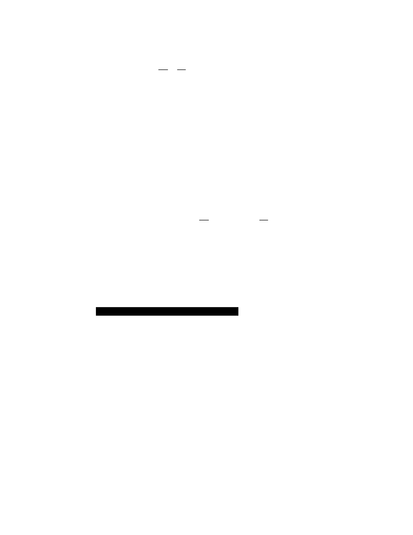
In the first stage, the algorithm computes potential regions within the image from which
patches can be extracted are computed. Given an image , the total number of potential patch
zones, 𝑍, is defined as:
𝑍(𝑥) = 𝑤C × ℎC .
(4. 25)
𝑤‘ℎ‘
Z essentially denotes the number of unique patches (slices) that can be extracted from 𝑥 without
any overlap. To extract these patches, the algorithm first defines a set of coordinates that
represent the top-left corner of each patch. Let 𝐶be such a set of coordinates:
𝐶(𝑥) = {(𝑖. 𝑤‘, 𝑗. ℎ‘) | 𝑖 = 0, . . . , 𝑤𝑤‘C − 1; 𝑗
= 0, . . . , ℎℎ‘C − 1} (4. 26)
Each coordinate in 𝐶 represents the starting point of a patch. For a given coordinate (𝑖, 𝑗), the
patch, 𝑃95, can be defined as:
𝑃 ,
(4. 27)
where 𝑃95 is a matrix representation of the patch starting at coordinates (𝑖, 𝑗).
Theorem 1 – Patch Extraction Completeness
For an image 𝑥 of dimensions (𝑤C, ℎC) and a patch size 𝑐, by utilizing the coordinates
set 𝐶 and the extraction method defined in Equation 4.27, the entire image 𝑥 can be
decomposed into 𝑍 non-overlapping patches, effectively ensuring that every pixel in 𝑥 is
represented in the set of patches without redundancy.
Proof of Theorem 1

•Non-Overlap: Given that each patch starts at a distinct coordinate from 𝐶 and extends 𝑤‘
pixels in width and ℎ‘ pixels in height, there's no possibility of overlap between patches
as 𝐶 has been defined with non-overlapping intervals.
•Complete Coverage: Considering the definition of 𝑍(𝑥) and 𝐶(𝑥), the entire image 𝑥 is
partitioned into 𝑍 patches, each of dimensions (𝑤‘, ℎ‘). This means, there is no pixel in
𝑥 that is not contained within a patch.
The core idea of the PROSIS algorithm rests on the belief that by rearranging these
patches based on certain indices or measures, one can expose significant features to the neural
network early in the training process, potentially expediting convergence and improving
generalization. This makes Theorem 1 significant for several reasons. As we transform images
into non-standard forms like rearranged patches, it's pivotal to ensure data integrity – that no data
is lost in this transformation. This theorem guarantees that all original information from the
image is retained in its patch representation. Additionally, this theorem ensures a consistent
methodology to decompose any image into a standardized set of patches, providing uniformity in
the transformation process. Another significance is the reversibility of the operation. Ensuring
every pixel is accounted for and that patches don't overlap provides the possibility to reconstruct
the original image, critical for potential backtracking, visualization, or debugging processes.
Stage 2: Patch Generation
At this stage, the algorithm takes the original sample, and the coordinates established in
the previous stage as inputs and breaks up the original image 𝑥 into equal sized patches (Figure
4.14). Based on the coordinate set 𝐶(𝑥) given in Equation (50), each coordinate pinpoints the
top-left corner of a patch. Iterating through each coordinate in 𝐶, patches 𝑃95 are extracted. This
procedure ensures every patch is of the defined size 𝑤‘, ℎ‘ and covers the entirety of the image.
Using the coordinate set and the patches 𝑃95 can be systematically extracted. Let 𝑃 be the
set of all patches:
𝑃
distinct patches, each with dimensions 16x16.
It is vital to generate non-overlapping patches. Overlapping could cause redundancy and
correlated features which might not be very helpful in the training phase, potentially leading to
overfitting or underfitting. Non-overlapping patches ensure that each section of the image is
treated as a unique entity, providing a diverse range of features to the algorithm.
Theorem 2: Non-Overlap Integrity
Given an image 𝑥 and non-overlapping patches list 𝑃, the union of all patches is equal to
the original image.
Proof of Theorem 2
Consider the image 𝑥 partitioned into non-overlapping patches 𝑃. Each patch 𝑃95 ∈
𝑃 is defined over a distinct set of pixels of x. Thus, the union of all patches will account
for every pixel in 𝑥 without repetition. Mathematically, this is stated as follows:
𝑥 = ˙ 𝑃95
(4. 29)
9,5
This theorem ensures that by breaking down an image into non-overlapping patches and
subsequently processing (or reassembling) these patches, the entirety of the original image's
information is preserved. Such an assurance is paramount when manipulating or reordering
patches, as it implies that no image information is lost or unduly replicated during the process.
Practical Implications and Utilization
With the patches 𝑃95 obtained, various transformations, including reordering based on a
specific criterion, and new input construction can be applied. These transformations aim to
emphasize specific features or characteristics of the image data, enhancing the learning model's
ability to discern patterns and improve overall training efficiency. The next stage will delve
deeper into how these patches can be assembled construct two types of inputs that are used to
enhance feature extraction [20].
Stage 3: Patch Ranking and New Sample Construction
Having generated distinct patches in Stage 2, we now enter the third stage which
essentially revolves around rearranging these patches in an optimized manner to maximize the
feature visibility. This not only involves a ranking system based on some predetermined measure
but also an effective methodology to reconstruct these patches into a sample. The reconstruction
process is realized in both 2D, and 3D space, with the latter introducing the concept of
volumization.
Patch Ranking Using Standalone Measures
A measure 𝑀 is specified to quantify a certain characteristic or property of the patch. As
detailed in the previous section, this measure can be of standalone or distance type. A standalone
metric acts as a function that maps a given patch 𝑃95 to a real number 𝕽, signifying its rank.
Mathematically, this is represented as:
𝑀: 𝑃95 → ℜ
(4. 30)
Patch Ranking Using Distance Measures
For distance metrics, the formulation is slightly more intricate, given the comparative
nature of these metrics. When employing distance measures, an essential step is the identification
or specification of a reference patch , 𝑃[#F, against which all other patches are compared. This
reference point serves as a baseline, providing context to the subsequent computations and
facilitating a consistent comparison across the set of patches in the image. Given the reference
patch and a patch 𝑃’" such that 𝑃 𝑃’" , the metric assigns a real number, 𝕽,
symbolizing the distance or similarity between them. Mathematically:

𝑀: 𝑃[#F, 𝑃95 →
ℜ
(4. 31)
Reference Patch in Distance Measures
The distance measures often require a point of reference, 𝑃[#F, to assess the relative
similarity or dissimilarity of other patches. If this is not specified, the algorithm by default
chooses the patch with the lowest entropy partly because a lower entropy value signifies that the
patch possesses lesser variability. Such patches, with their homogeneity, act as a more stable and
consistent baseline for comparison. Using a patch of low entropy as a reference ensures that the
distance metrics computed provide a relative measure of complexity with respect to a simple,
consistent structure.
Algorithm 4.1. Algorithm PROSIS (Patch Reordering Optimization for Structured Input
Sequencing) for Generating 2d and 3d Data.
Input: Image 𝑥 with dimensions (𝑤C, ℎC), Patch size 𝑤‘, ℎ‘ ,Metric M, Optional
reference patch 𝑃[#F.
Output: Reordered list 𝑂 of patches from 𝑥 .
Step 1: Patch Zone Proposals Generation • Compute the total number of
potential patch zones: 𝑍(𝑥) = H,×:,
H-:-
•2. Define a set of coordinates 𝐶(𝑥) for the top-left corner of each patch:
𝐶‘ ‘ 𝑤𝑤‘C
ℎℎ‘C
•3. Extract each patch using:
𝑃

Step 2: Metric Application and Patch Ranking
If 𝑀 is standalone:
§Compute the metric value for each patch: 𝑟95 = 𝑀(𝑃95)
§Sort patches based on rank to form the list 𝑂. Else if 𝑴 is a distance
measure:
§If 𝑃[#F is not specified, o Determine the patch with the lowest entropy and
set it as 𝑃[#F.
§Compute the distance between each patch and the reference: 𝑑95 =
𝑀 𝑃95, 𝑃[#F
§Sort patches based on 𝑑95 to form the list 𝑂. Step 3: Construct the
Reordered Sample
§Use the ranked list 𝑂 to assemble the reordered sample 𝑥′R+.
§Or to build a 3D volumetric representation 𝑥′a+.
End
For instance, if we had chosen a patch with high entropy (high variability) as a reference,
the results could become more subjective, based on which complex pattern was chosen. On the
other hand, a patch with low entropy, being more uniform, provides a neutral starting point.
Thus, it aids in drawing more objective comparisons among the various patches, essentially
highlighting the deviation of each patch from a simpler, uniform pattern.
Sample Reconstruction
Once the metrics have been applied, and each patch has been assigned a rank, an ordered
set 𝑅 is generated.
𝑅 = {𝑟4, 𝑟R, … , 𝑟0}
4. 32
This set is then arranged in ascending or descending order based on the goals of the application
and the nature of the chosen metric.

The set 𝑅 is used reconstruct a sample that can be used to train alongside the original
input or by itself. The form of this reconstruction can be in 2𝐷, or 3𝐷 based on application
needs.
2D Reconstruction (PROSIS-2D)
Given an original sample 𝑥, when constructing a 2D augmented counterpart, the patches
are positioned adjacently, maintaining the sequence from the ordered patch list R. This strategy
results in a continuously structured image that retains the dimensions (𝑤C, ℎC) of the original,
but the interior patch configurations have shifted based on the chosen metric's evaluation.
Mathematically, the 2D reconstruction can be represented as:
𝑖 ℎC𝑗
𝑅R+(𝑖, 𝑗) = ˝˛𝑤‘ˇ × ˛ℎ‘ˇ × ˛ℎ‘ˇ—b9 8IJ H-,5 8IJ :-c ,
(4. 33)
where 𝑖 = 0 𝑡𝑜 𝑤C − 1 𝑎𝑛𝑑 𝑗 = 0 𝑡𝑜 ℎC − 1.
3D Volumization (PROSIS-3D)
In the 3D Volumization method, each patch from 𝑂 takes its position as a distinct layer
within a 3D space. The patches are sequentially stacked along the z-axis, thereby introducing
depth. While this volume retains the patch dimensions 𝑤‘, ℎ‘ for the x and y axes, it expands to
accommodate Z layers along the z-axis. The resulting 3D structure, 𝑅a+, can be represented as:
𝑅a+(𝑖, 𝑗, 𝑘) = 𝑅[𝑘](9,5),
(4. 34)
where 𝑖 = 0 𝑡𝑜 𝑤‘ − 1 , 𝑗 = 0 𝑡𝑜 ℎ‘ − 1 𝑎𝑛𝑑 𝑘 = 0
𝑡𝑜 𝑍 − 1. In the output, the 𝑥 and 𝑦 axes define the spatial distribution of each
patch, while the z-axis signifies the depth of the volume.

By default, 𝑅a+ has a shape of (𝑤‘, ℎ‘, |𝑍|).
Complexity Analysis PROSIS
In the initial phase of Patch Zone Proposal, calculating the total potential patch zones per
image is straightforward and only requires constant computational time 𝑂(1). Determining the
coordinates set 𝐶(𝑥) equates to performing two linear operations dependent on the image’s
dimensions juxtaposed with the chosen patch size. The complexity of this step is 𝑂(H, × :,)
H-:-
which is simplified to 𝑂(𝑍) where 𝑍 = H, × :, is the total number of patches per image.
H-:-
Subsequently, as each patch is extracted, the computational demand is 𝑂(𝑍 × 𝑤‘×
ℎ‘).
Transitioning to the Patch Assessment and Ranking phase if the chosen metric
𝑚 is a standalone, each patch's metric computation remains consistent, each taking O(1) time.
Thus, for all patches, the complexity aggregates to 𝑂(𝑍). However, when m serves as a distance
measure, identifying the patch with the most minimal entropy demands a computational
complexity of 𝑂(𝑍). Calculating the distance between each patch and the reference is also in
order of the total number of patches. The subsequent sorting for both standalone and distance
metrics retains a complexity of 𝑍𝑙𝑜𝑔 𝑍.
Lastly, during the Sample Construction phase, the complexity is linear with the number of
patches, 𝑂(𝑍), for both 2D and 3D samples. Combining all, algorithm PROSIS’s complexity of
processing every sample in a dataset containing 𝑁 samples is:
𝑂(𝑁 × (𝑍 × 𝑤‘× ℎ‘+ 𝑍𝑙𝑜𝑔 𝑍) (𝑁 × 𝑍
× 𝑤‘× ℎ‘).
(4. 35) The space complexity on the other hand is determined by the
number of patches generated; 𝑂(𝑁 × (𝑍 × 𝑤‘× ℎ‘)). Additionally, storing
the standalone or distance rank of each patch in an image introduces an overhead of 𝑂(𝑍).
This list can be sorted in place without requiring additional storage. Combining all, the space
complexity of algorithm process is:
𝑂(𝑁 × (𝑍 × 𝑤‘× (𝑁 ×
𝑍). (4. 36)
Algorithm PROSIS presents a computational complexity shaped majorly by the patch
extraction process and sorting operation. Its space demands primarily hinge on the storage of
these patches. These complexities serve as invaluable touchstones, anticipating resource
requirements, especially when training on a set of large images or processing an ensemble of
images concurrently.
Summary
This chapter discusses implementation of Deep-CLO framework, designed to optimize
deep learning using CL techniques and two unique preprocessing algorithms. The framework
takes inspiration from human cognitive development and learning, particularly curriculum
learning, to enhance CNN and mitigate challenges such as their vulnerability to adversarial
attacks. The framework's perspective views digital images as 2D random variables with each
pixel acting as an independent realization. This view assists in analyzing training dataset’s innate
properties, fostering deeper insights into individual samples and their interconnections.
In alignment with our thesis statement, the upcoming chapters seek to critically evaluate
the propositions made about deep learning optimizations. We strive to validate the assertion that
the characteristics of a training set, assessed using metrics like entropy, and the intricate
statistical relationships both between samples and between patches within images, can be
adroitly harnessed to refine deep learning processes. By doing so, we aim to achieve enhanced
feature extraction, superior model generalization, and a fortified defense against adversarial
interferences.

CHAPTER 5
APPLICATION OF DEEP-CLO IN IMAGE CLASSIFICATION: A COMPARATIVE
STUDY OF CURRICULUM LEARNING
Introduction
Curriculum Learning (CL), though grounded in principles of human learning, remains
largely on the fringes of mainstream deep learning methodologies. While its promise holds
immense potential, the journey from theoretical constructs to practical applications in the context
of real-world machine learning models is remains a challenge [125].
This research stands at the crossroads of this transformative idea and its practical
realization in the domain of image classification. Given the rich and multifaceted nature of visual
data, we navigate the intricacies of CL for efficient model training.
Our aim with this chapter is:
•From theory to practice: We highlight our pioneering efforts to bridge the gap between
the theoretical allure of CL and its practical implementation. We'll present our strategies
for integrating CL within modern ML frameworks, making it accessible and efficient for
broader adoption.

•Designing a tailored CL strategy for image classification: Crafting an effective and
efficient Curriculum Learning approach for image classification, elucidating the criteria
for determining sample complexity, sequencing strategies, and the symbiotic relationship
between CL and other optimization techniques.
•Real-world case studies: Dive deep into our implementations of CL in a range of image
classification scenarios using various benchmark datasets. This will provide an insightful
look into the challenges, innovations, and breakthroughs we experienced throughout this
research.
•Comparative analysis: Present results of our empirical study, contrasting the performance
of models trained using conventional paradigms against those trained using CL.
Related Work
This section provides an overview of pertinent research in the domain of CL, with a
specific focus on image classification. The goal is to situate our research within broader
academic literature, identifying both convergences and divergences.
Foundational Studies on Curriculum Learning
At the heart of Curriculum Learning is the philosophy borrowed from human educational
practices. Bengio et al. (2009) [19] were among the pioneers to introduce and formalize the
concept of Curriculum Learning in the context of deep learning. Their study underscored the
potential of CL in facilitating smoother optimization and better generalization. They found that
when neural networks are trained using a curriculum, the optimization landscape changes. This
staged training can help avoid local minima and guide the optimization towards better solutions.
They also found that a well-structured curriculum aids in preventing overfitting. By allowing the
model to first learn basic patterns and then incrementally introducing complexity, it encourages
the model to generalize better on unseen data. By drawing analogies to how humans and animals
learn, this study sets the stage for subsequent explorations in CL.

Their approach centers on error-based correction which leverages the model's error on
samples as an indicator of their difficulty or importance. By focusing on uniformly sampling
from the training set, the approach ensures that the model is continually exposed to and learns
from its mistakes, subsequently speeding up its learning trajectory. This is analogous to a student
repeatedly practicing problems they find challenging until they master the concept [19].
CL Methods Rooted in Sampling Strategies
Building on this foundational idea, a number of methods have been proposed [126] [127]
to sample , weigh and sort training samples. A series of works, such as those by Kumar et al.
(2010) [128] and Weinshall et al. (2018) [111], have delved into the mechanisms of weighted
sampling and data sorting. The weighted sampling technique assigns importance or difficulty
levels to each data sample, ensuring that more influential samples have a more significant impact
on the model's learning process. Meanwhile, data sorting strategies emphasize sequencing the
training data, often progressing from simpler to more intricate samples, thereby streamlining the
model's learning journey. Other work that rely on sampling strategies either require modification
of the objective function (Equation 2.1) with a term for sample valuation [128] or run training
procedure twice to obtain accurate representation of sample effectiveness. This sample valuation
plays a pivotal role in refining the model's learning trajectory, aligning the model updates closely
with the curriculum's objectives.
Another approach is a dual-training strategy which involves conducting the training routine
in two phases [125]. The initial phase ascertains the importance or difficulty of the training
samples, laying the groundwork for the subsequent phase. The second phase leverages these
insights to refine the curriculum.
Optimization Loss as a Criterion
Another notable criterion is the use of optimization loss, a strategy that has shown promise
in refining how training samples are presented to the model. Schaul et al.’s work [129]
demonstrated the potential of this criterion. Their research uses optimization loss to evaluate and

increase the replay probability of samples that have high expected-learning-progress. The
underlying philosophy of this approach is rooted in the understanding that samples which pose a
higher learning challenge – indicated by a greater optimization loss – typically offer more fruitful
learning opportunities for the model.
By focusing on challenging samples, this strategy can introduce biases, and the model is at
risk of overfitting to these specific instances, thereby compromising its generalization
capabilities on unseen data. Schaul et al. were aware of this and proposed a solution. They use a
weighted importance sampling method to counter bias of sampling [129].
Non-uniform Mini-batch Sampling
Traditionally, SGD and its variants often rely on uniformly sampled mini-batches for
training [63]. However, the realization that some training samples can be more informative than
others during different phases of training has led to the exploration of non-uniform sampling
strategies. The work of Loshchilov and Hutter [130] brings to fore this sampling strategy. Their
methodology departs from the conventional uniform approach, advocating instead for a
dynamically weighted sampling process. By doing so, they provide evidence to the observation
that not all samples contribute equally to the learning process at every stage of training. Some
data points, especially outliers or those that represent less frequent but crucial patterns, can often
be underrepresented in uniform sampling. Loshchilov and Hutter's approach ensures that such
data points receive adequate attention, allowing models to converge faster and attain better
generalization [130].
In a similar vein, Graves et al. [131] ventured into the realm of automatic curriculum
learning, particularly focusing on NLP applications when using Long Short-Term Memory
(LSTM) networks. LSTMs, with their inherent capacity to handle sequential data, are
particularly sensitive to the sequence and variety of training samples presented. In such contexts,
the mere act of non-uniform sampling can profoundly influence the training dynamics.
Graves and his colleagues introduced a unique mechanism to define a stochastic syllabus
for training: a non-stationary multi-armed bandit algorithm [131]. At its heart, the multi-armed

bandit problem is about exploration and exploitation. In the context of CL, this translates to the
dilemma of when to focus on familiar training samples (exploitation) and when to explore new,
potentially more challenging ones. By associating a reward signal with each training sample,
Graves et al. were able to dynamically adjust the probability of a sample being included in a mini
batch based on its historical contribution to the learning progress. This allowed for a more
adaptive and responsive training regimen, catering specifically to the nuances of NLP tasks.
Our Approach
In contrast to previous work, our method uses inherent characteristics of images to
discover optimal input paths. Using inherent characteristics of images as a basis is the main
aspect of the proposed approach. Why is this a promising idea for CNNs? There are several
reasons. First, inherent characteristics provide a natural ordering or hierarchy in the data. Just as
in human learning, where fundamental concepts form the base for more complex topics, the
inherent traits of images can create a structured pathway for machine learning.
Additionally, by grounding our approach in inherent characteristics, it ensures that the
curriculum is consistent and replicable. Different researchers working with similar data would
arrive at comparable curriculums, making results more consistent across different experiments.
Another salient advantage is the potential for enhanced efficiency in the learning process.
By introducing data in an order that mirrors its intrinsic structure, we find that neural networks
could achieve convergence more rapidly. Furthermore, these inherent characteristics can act as
discerning filters, sifting through the data to prioritize the most pertinent features. This can
significantly reduce the noise during the training phase, ensuring that models initially focus on
the most crucial patterns before progressing to complex variations.
A curriculum grounded in these inherent features might also bolster the model's
generalization capabilities. Establishing an understanding rooted in core, intrinsic features could
set a robust foundation for the model, enhancing its performance when faced with unseen data.
Each dataset or domain possesses its unique inherent characteristics. By spotlighting these, the

learning trajectory becomes finely tuned to the specific nuances of the dataset. This adaptability
equips the model to tackle diverse challenges, making the emphasis on inherent characteristics
not just a strategic choice, but an indispensable element for the success of our approach. The end-
toend training pipeline is depicted in Figure 4.11 and presented in Algorithm 5.1.
As discussed in the previous chapter, the algorithm begins by assessing and ranking
training samples in batches, using metrics that highlight essential patterns within the data. By
ranking samples based on difficulty or importance, the model becomes sensitive to data
variations early in training. The samples are then sorted based on their rank. This sorting step
refines the sample order, creating a syllabus that aligns with the nuanced relationships within the
data. The model then trains on this syllabus for a baseline number of iterations, enabling an
evaluation of syllabus effectiveness through average loss and syllabus-to-baseline loss ratio. A
fitness signal is derived to guide whether to continue with the syllabus, terminate, or recalibrate
based on auxiliary metrics. This process, from ranking to fitness evaluation, constructs a data-
specific, adaptive training pipeline that makes training more efficient by aligning learning with
the dataset’s inherent features.
Algorithm 5.1. Curriculum Training of the CNN Network. Here, At Least Two M Values, a
Primary Measure, And Backup Measures, from Table 2 Are Pre-Specified.
Inputs: Training set 𝑫, Metric 𝑴, Baseline Iteration Span π, Baseline Benchmark β
Outputs: Trained model G-
Stage I: Assessing and Ranking Training Samples
1. Extract batch 𝑩 = {𝒙𝟏, 𝒙𝟐, … , 𝒙𝑴} ⊂ 𝑫
2. Rank samples in B using metrics from Table 1.
3. Generate rank set R such that 𝜺𝒙𝟏 ≤ 𝜺𝒙𝟐 ≤ ⋯ ≤ 𝜺𝒙𝑴
Stage II: Sorting Batches of Samples
1. Initialize reference sample 𝒙𝒓𝒆𝒇 = 𝒙𝟏
2. For each sample 𝒙𝒌 :

oRank 𝒙𝒌 based on metric mm and relation to other samples in B.
oIf metric mm uses mutual information II:
§Compute mutual information rank 𝜺 of 𝒙𝒌 with respect to .
§If using ascending order, update 𝒙𝒓𝒆𝒇 based on minimal ε.
3. Create syllabus 𝜴 based on mutual information ranks.
Stage III: Syllabus Fitness Evaluation
1. Train network on 𝑫 for π iterations using syllabus Ω.
2. Compute average loss: 𝜷𝜼→𝑺
3. Compute syllabus-to-baseline loss ratio: λ
4. Determine fitness signal 𝒇𝒔:
oIf λ≤1, set 𝒇𝒔 𝒕𝒐 Continue. o If λ exhibits no advantage, set 𝒇𝒔
to Terminate.
oOtherwise, set 𝒇𝒔 to Adaptive Rerun and recalibrate with an
auxiliary metric. Return G-
Experimental Setup
We heavily relied on state-of-the-art models and common benchmark datasets to validate
our approach.
Benchmark Datasets
In the expansive field of image classification, datasets serve as the bedrock upon which
algorithms are trained, validated, and tested. Their quality, diversity, and volume directly
influence the performance and robustness of the models. For this research, we used several
datasets, each offering its own challenges and nuances.
Synthetic 2D Geometric Images Dataset
One dataset we used to for comparative analysis of our CL approach to the foundation
study highlighted above is the Synthetic 2D Geometric Images Dataset [132]. Unlike many
popular image datasets which are comprised of real-world photos, this dataset is synthetic dataset
of abstract geometric shapes such as square, circle and triangle. Each shape varies in terms of

size, orientation, position, and color, lending the dataset both diversity and complexity. In the
broader spectrum of this research, the Synthetic 2D Geometric Images Dataset serves a twofold
purpose. It offers a testing ground to evaluate how CL strategies fare in the domain of abstract
pattern recognition. Secondly, it provides a comparative framework to the foundational study of
Bengio et al. which uses a similar dataset.
CATS vs DOGS Dataset
The CATS vs DOGS dataset [133] primarily focuses on a binary classification task
involving images of cats and dogs . Each image in the set is either a dog or a cat and encapsulates
myriad complexities - including poses, diverse backgrounds, fluctuating lighting conditions, or
the different breeds, making this dataset an appropriate choice for research delving into binary
image classification tasks (Figure 5.2). We use this dataset due to its simplicity rendered by just
two distinct classes to finetune our methodology.
CIFAR10 Dataset
The CIFAR-10 dataset [134] consists of 60,000 colored images, each of size 32 by 32
pixels, uniformly distributed over 10 different classes. These classes encompass a diverse set of
items: airplanes, cars, birds, cats, deer, dogs, frogs, horses, ships, and trucks (Figure 5.3). Each
class has an equal representation with 6,000 images. From the total images, 50,000 are
designated for training and the remaining 10,000 for testing.
The images in this dataset are of a relatively low resolution. This characteristic presents a
challenge because models need to recognize and categorize objects without relying on the
extensive details available in high-resolution images. Furthermore, the variety within the dataset
ensures that models need to be adaptable. They must be able to differentiate not just between
completely different categories, such as trucks and frogs, but also between categories that might
have similarities in certain images, like cats and dogs.

For our research, the CIFAR-10 dataset was specifically chosen for a detailed exploration
of our approach. Given its volume and multi-class nature, it stands as an optimal benchmark for
in-depth analysis. Another important feature is its reflection of real-world imaging scenarios. The
dataset maintains a balanced representation, ensuring no class bias. Moreover, it showcases
images that aren't overly idealized, capturing objects under varied conditions, including different
angles, scales, and lighting. This ensures that models trained on CIFAR-10 are adept at
Figure 5.3. Samples Taken from the CIFAR10 Dataset.
interpreting images in diverse real-world scenarios, not just under controlled conditions. The
dataset's consistent adoption in both academic and professional settings underscores its
significant value in training and evaluating image classification models.
CIFAR100 Dataset
The CIFAR-100 dataset [134], a successor to CIFAR-10, encompasses 60,000 colored
images, each sized 32 by 32 pixels (Figure 5.4). Unlike its predecessor, which contains 10
classes, CIFAR-100 expands its scope to cover 100 classes – 600 images for each. This dataset
further structures its classes by categorizing them under 20 superclasses, offering a hierarchical
organization that can be utilized for multi-tiered classification exercises.
The core challenge with CIFAR-100 lies in the intricacy of its classes. It demands
classifiers to discern finer nuances and more subtle features. For a comparative example, while
CIFAR-10 might focus on distinguishing broader categories such as birds from airplanes,
CIFAR-100 delves deeper, requiring differentiation among varied species of birds or diverse
aquatic animals.
Figure 5.4. Samples Taken from the CIFAR100 Dataset.
In our study, we use this dataset as a benchmark to probe the adaptability and scalability
of our proposed approach. One of the key questions in machine learning, particularly in
classification, is the generalization capability of models as the number of classes grows. With its
granular set of 100 classes, the CIFAR-100 provides an opportunity to address this question.
ImageNet Dataset

The ImageNet dataset [99] serves as the main benchmark dataset in the world of
computer vision. This dataset has had a transformative influence on the field of deep learning,
especially in image classification tasks [135], [136], [137], [138].
ImageNet is an intricate assembly of millions of annotated images spread across
thousands of categories. With more than 14 million images, this dataset encompasses over 20,000
categories, with each image annotated with detailed bounding box information, providing both
category and object localization (see Figure 5.5).
The most well-known aspect of ImageNet is the ImageNet Large Scale Visual
Recognition Challenge (ILSVRC). The ILSVRC is a competition where research teams evaluate
their algorithms, pushing the boundaries of what's achievable in image recognition tasks.
Notably, the 2012 edition of the ILSVRC marked a turning point in the field of deep learning,
with Alex Krizhevsky, Ilya Sutskever, and Geoffrey Hinton's CNN known as AlexNet,
significantly outperforming traditional computer vision methods [135].
In practical terms, ImageNet has served as the training ground for many of the state-
ofthe-art models in deep learning, from the early AlexNet to more recent architectures like
ResNet, EfficientNet, and many others. These models, pre-trained on ImageNet, are often used
as starting points for transfer learning, benefiting numerous applications beyond just image
classification.
Figure 5.5. Samples Taken from the ImageNet (ILSVRC12) Dataset.
In the context of this research, the use of ImageNet provides a robust platform to evaluate
the impact and effectiveness of our proposed approach. Given its complexity and breadth, any
improvements in training efficiency or model generalization achieved here could have broad
implications for the wider deep learning community.
State-of-the-art CNN Architectures
Advancements in deep learning have led to the development of several, current and past
state-of-the-art (SOTA) CNN architectures. Each architecture is designed with unique features
tailored to achieve superior performance. For our study, we selected a collection of these leading

models, given their widespread acclaim and proven performance in image classification. Below,
we discuss all architectures used in our study.
EfficientNet Family
EfficientNet represents a pioneering shift in CNN architectures [139]. Its core innovation
lies in the employment of a novel model scaling method (Figure 5.6) [140]. Unlike conventional
approaches where only one dimension (depth, width, or resolution) of the network is scaled,
EfficientNet utilizes compound coefficients. These coefficients are determined based on a
systematic search to scale all three dimensions, allowing the model to achieve a more structured
and balanced scaling.
Table 5.1. Summary of Dataset Used in this Study.
Dataset Name Training Set Count Test Set Count
2D Geometric Shapes 72000 18000
Cats’ vs Dogs 20000 50000
CIFAR10 50000 10000
CIFAR100 50000 10000
ILSVRC2012 1281167 100000
From a performance standpoint, EfficientNets have set new benchmarks in tasks like
image classification [140]. As reported in Tan & Le (2019) [140], EfficientNets not only
achieved state-of-the-art results on ImageNet but have accomplished this feat with impressive
efficiency. Specifically, the EfficientNet-B7 model achieved a top-1 accuracy of 84.4% while
having 66M parameters, in stark contrast to previous architectures like GPipe [141] which
achieved a top-1 accuracy of 84.3% with 557M parameters [140]. This drastic reduction in model
parameters without compromising on accuracy underlines the architectural innovations of the
EfficientNet family. Furthermore, this architecture is not limited to just image classification.
Recent studies and applications have showcased its robust transfer learning capabilities across a

plethora of datasets and tasks, reinforcing EfficientNet's esteemed position among CNN
architectures.
FixEfficientNet-L2
In addition to EfficientNet-B0 and B7, our experimentation also involved
FixEfficientNet-L2 variant [142], which garnered significant attention by surpassing SOTA
accuracy benchmarks in 2019 [142]. Emerging as an evolution over the foundational EfficientNet
architecture, FixEfficientNet-L2 integrates a newer weight update mechanism known as FixRes
[142]. This update strategy allows the model to fine-tune the resolutions during the training
process. This design choice, among others, has elevated FixEfficientNet-L2 to the pinnacle of
performance, making it highly competitive in the ImageNet ILSVRC 2012 benchmark.
ResNet and its Variants
ResNet (Residual Network), as introduced by He et al. [8], marked a significant shift in
the understanding and design of deep neural networks. These architectures are characterized by
their residual blocks (Figure 5.7), allowing the training of much deeper networks. These blocks
leverage skip connections or shortcuts that bypass one or more layers. This design was primarily
formulated to tackle the vanishing gradient problem that plagued deep networks [143], making
training them almost infeasible. Using these residual blocks, ResNet managed to train networks
with a depth of up to 152 layers, significantly deeper than what was considered feasible before its
introduction.
The ResNet architecture family was the first to dispel the common belief that network
depth is proportional to overfitting. They illustrated that deep networks can, in fact, reduce both
training and validation errors. In our research, we explored the foundational ReseNet-50 two
deeper variants, BiT-L
(Big Transfer-Large) [144] and ResNeXt [145].
BiT-L

Big Transfer (BiT-L) [144] is rooted in the idea of pre-training on large datasets and then
transferring the learned knowledge to other tasks. This model underscores the importance of
transfer learning and its potential to accelerate training processes, especially in scenarios with
limited data.
One of the outstanding attributes of BiT-L is its resilience when training with scarce data.
In many real-world scenarios, obtaining a large, labeled dataset is challenging and expensive.
BiT-L circumvents this impediment by leveraging its pre-trained knowledge, enabling robust
performance even with limited target data. Our experiments with BiT-L aimed to discern its
adaptive capacity and the efficiency of its transfer mechanism across diverse curricula [21].
ResNeXt
An augmentation to the ResNet architecture, ResNeXt [145] introduces the concept of
cardinality as an additional model dimension, which represents the number of parallel pathways
or branches. This parameterization enhances the representation power of the model without
significantly increasing its complexity. Empirical findings suggest that increasing cardinality can
be more effective in augmenting the model's expressive capability than merely deepening or
widening it.
This design innovation does not just bolster model performance but achieves this without
an exponential surge in parameters or computational overhead. In the context of our study,
ResNeXt offered a unique lens to understand how varying model architectures, especially those
with distinct cardinalities, interact and perform under distinct curriculum designs.
Inception (GoogleNet)
Inception or GoogleNet, as it's colloquially known, was the winner of the ILSVRC
challenge in 2014, and it significantly transformed CNN designs that followed it [146]. The key
innovation behind this architecture is Inception module (Figure 5.8) that
captures spatial hierarchies effectively.

The motivation behind this design was to recognize patterns at multiple scales within the
same layer. The Inception module embodies parallel operations with filters of varying sizes
(1 × 1, 3 × 3, 5 × 5) and max pooling. Post these operations, the outputs are concatenated
and sent to the next layer. This means, at each layer, the model is facilitated to recognize patterns
of different spatial extents. This multi-scale recognition makes it adept at grasping varied
complexities in images. Additionally, the Inception architecture used a unique feature of 1 × 1
convolutions, or what is termed as network-in-network. These 1 × 1 convolutions, though
seemingly trivial, play a pivotal role in reducing dimensionality, thereby making the
computations more efficient without sacrificing the network's representational power.
In our dissertation, we leveraged the Inception v2 variant, an optimized iteration of the
base architecture. Inception v2 builds upon the foundational concepts while amalgamating new
strategies such as factorizing convolutions and improved normalization techniques [146]. This
refinement enhances its ability to generalize across datasets and provides a competitive edge in
terms of performance metrics. Exploring this model within our study offered a chance to discern
how this unique architecture fares under various curriculum training and evaluation conditions.
MobileNet Family
MobileNet architectures are tailor-made for efficiency [147], especially in contexts with
strict computational constraints like mobile and embedded devices. Its design philosophy stems
from the need for lightweight models that don't compromise on performance.
Depth-wise separable convolutions serve as the backbone of their design. By
deconstructing the standard convolution into two stages - a depth-wise convolution followed by a
1 × 1 point-wise convolution - MobileNets achieve dramatic reduction in computational
overhead. This innovative process not only lessens the number of required computations but also
manages to largely retain the representational power typical of more demanding architectures. It
integrates techniques like depth-wise convolutions and hardware-aware network architecture
search, ensuring a fine balance between accuracy and speed.

MobileNet v3
The third iteration, MobileNet v3 [148], assimilates lessons from its predecessors and
integrates novel design enhancements, further solidifying its position in efficient computing. A
pivotal enhancement in v3 is the Hardware-Aware Network Architecture Search (NAS) [148]. In
this approach, the architecture isn't solely optimized on theoretical computational benchmarks.
Instead, it's sculpted with an acute awareness of the practical hardware dynamics it's intended to
operate on. This real-world attunement ensures the model's performance remains optimized in
tangible deployment scenarios, not just in lab settings.
Further enriching the v3's architecture is the introduction of the h-swish activation
function [148]. This function, a hardware-friendly iteration of the more traditional Swish
function [149], has demonstrated exceptional performance, particularly in mobile contexts. The
function exemplifies the intricate balance of optimizing computational efficacy while ensuring
mathematical robustness.
Incorporating MobileNet v3 into our investigation presented an opportunity to delve into
the performance of an architecture specifically designed for efficiency under computational
constraints. By subjecting it to various curriculum strategies, we assess how well our proposed
algorithms balance model performance with computational efficiency.
VGG Models
The VGG models [7], developed by the Visual Geometry Group [150] at the University of
Oxford, introduced a series of convolutional neural networks that emphasized the role of depth in
achieving high performance. With configurations ranging from 11 to 19 layers, these models
have played a pivotal role in understanding the implications of depth in CNNs. The design
simplicity, characterized using small convolutional filters and a consistent architecture
throughout, made VGG models a valuable benchmark in the deep learning landscape,
particularly for image classification tasks.
VGG-19

For our study, we zeroed in on the VGG-19 variant, leveraging its depth to assess
curriculum learning's impact on such architectures. With 19 layers, VGG-19 represents one of the
deeper variants available. Investigating such a deep network can provide insights into how depth
impacts training dynamics and final model performance. Does the depth augment its capability to
grasp a curriculum better, or does it introduce unforeseen challenges? This was among the many
questions we aimed to address. Given the model's depth, it was crucial to understand if such an
architecture benefits from a structured learning approach or if it faces challenges unique to its
design.
Additional Metric
Validation of classification models typically branches into two distinct stages: the training
phase (or learning) and the testing phase. Their interplay is essential to understanding the
maturity of a model.
In the training phase, the primary focus is on optimizing the classification models’
parameters. Hence, evaluation metrics such as loss over time (or accuracy over time) are
essential in gauging the classifier's evolving efficacy as a function of training iterations.
In the testing phase, we pivot our attention to the efficacy of the model when it confronts
unseen data. This essentially captures the generalization performance of the model. It's the
ultimate test, challenging the model to extrapolate its learned features to new data. Here, the
metric morphs into an evaluator, assessing how well our classifier has generalized from its
training. In addition to the metrics discussed in Chapter 3, we also report training and testing
trends as measured by loss or accuracy.
Experimental Results
In this section we present a summary of published results that showcase the applicability
of the proposed approach [20], [22], [23], [36], [151].

Comparison with Foundational Study
Bengio et al. [19] conduct their study of curriculum learning using synthetic 2D images,
primarily shapes, to validate the impact of structured training on neural networks. In a similar
vein we employed datasets of different complexities to probe the nuances of our curriculum
learning approach. Their dataset comprised of GeomShapes, showcasing a range of geometrical
shapes, and BasicShapes, a more constrained subset focusing on squares, circles, and equilateral
triangles. The relative simplicity of BasicShapes compared to GeomShapes allowed them to
experimentally assess the advantages of starting with a simpler curriculum before transitioning to
more complex data.
In our investigation, we employed a similar model – a multi-layered neural network with
three hidden layers. This architecture was trained using SGD to minimize the negative
conditional log-likelihood. However, our training approach diverged somewhat. We avoided the
two-step curriculum Bengio's team used. Instead of starting with BasicShapes and transitioning
at a switch epoch to GeomShapes, we trained our model directly on the entirety of the
GeomShapes dataset. For comparison, we juxtaposed our results with the baseline they
established — a scenario where the neural network is trained solely on the GeomShapes dataset.
Their research demonstrated that a curriculum that splits the training time between the
BasicShapes dataset and the GeomShapes delivers better generalization than training without a
curriculum. Interestingly, when they blended the BasicShapes and GeomShapes datasets for
noncurriculum training, the outcomes were less optimal compared to the curriculum-based
strategy.
As illustrated in Figure 5.9, our mutual information-based CL strategy on the blended
dataset aligns closely with the findings of Bengio et al. This not only reaffirms the inherent
advantages of curriculum learning but also emphasizes its potential in expediting model
convergence, surpassing conventional training methods.
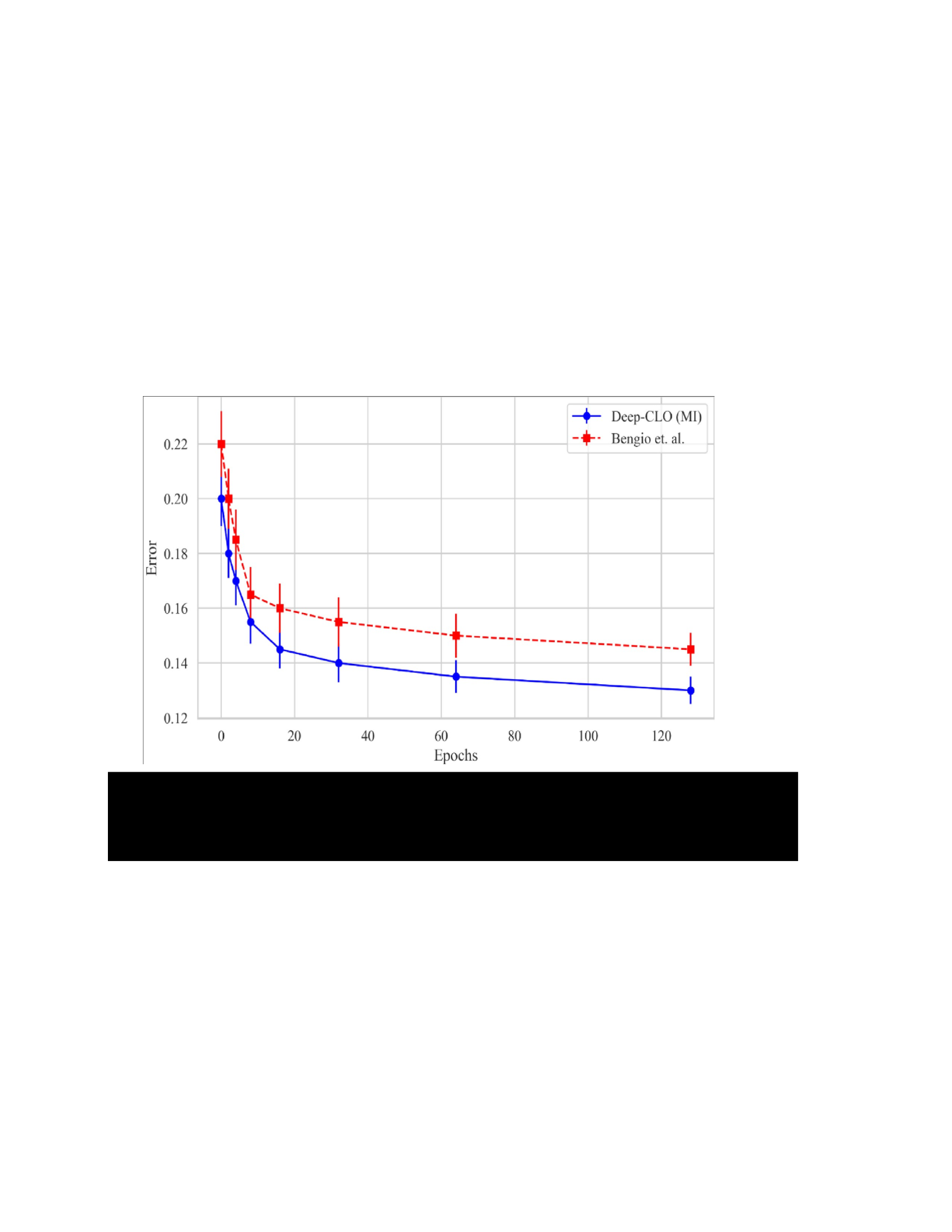
Experiments on SOTA Model Architectures and Benchmark Datasets
Training Setup
All models were trained using open-source TensorFlow implementations of our
framework. Each network is first evaluated on the corresponding datasets to create baseline
reference performance metrics for comparison. For each network we used stochastic gradient
descent (SGD) optimizer and its variant, Adaptive moment estimation (Adam) [79], a fixed
momentum of 0.9, batch size of 8, and an exponentially decaying learning rate with factor 0.94
starting at 0.01. For the rest of the training, recommended configurations by respective authors
were used. We report empirical results gathered by training each network for at least 1 million
iterations. All learning parameters and environment are fixed, with varying networks, learning
methods (curriculum vs no-curriculum) and optimizers, to rule out other factors of influence.
Testing Scenarios
The standard testing scenario of a classification task is to train the models using a portion
of the dataset and then test it in previously unseen, held out test set. This setting is preferred and
Figure 5.9. Comparison of Training Errors Over Epochs: Deep-CLO (MI) Vs. Bengio et al.'s
Approach Using a Multi-Layer Perceptron. Both Methods Show a Decline in Error Rates Over
Epochs, Highlighting the Effectiveness of Curriculum-Based Strategies. Our MI-Based Syllabus
Consistently Outperforms the Foundational Study Across the Epochs.

able to clearly measure the generalizability of the model with and without the proposed method,
so we evaluate our approach under the standard testing scenario.
Results and Analysis
This section presents a systematic evaluation of previously discussed models trained
using various curriculum strategies. The goal is to compare their performance against established
baselines on the respective datasets.
CIFAR10 Training Results
First, we evaluated training performance of all models using various curriculum
strategies and compared the results to the baseline, SOTA performance of each model on the
corresponding dataset. We use the total loss, which is the sum of cross-entropy and regularization
losses, as the primary evaluation criteria of the impact of each CL strategy on training. The
results are depicted in Figure 5.10, Figure 5.11, Figure 5.12, and Figure 5.13.
With most curriculum strategies, a large improvement in training performance over the
baseline is observed. This shows that the proposed method accelerates training in agreement with
prior theoretical investigation [19], [111].
EfficientNet
When trained using the standard SGD optimization, EfficientNet-B7 exhibited notable
enhancements under our CL strategies. For instance, as depicted in Figure 5.10 (left), 15.6%
absolutes percentage improvement is noticed in reducing the training loss when training using
the mutual information (MI) syllabus on CIFAR10 dataset. The improvement is consistently
observed on the other curriculum strategies. Similar trends are observed with all curriculum
strategies outperforming the baseline, and the improvements are statistically significant.
Similarly, FixEfficientNet mirrored the training performance improvements of its B7
counterpart (Figure 5.11). Under mutual information (MI) syllabus, this model managed to
achieve a similar performance of 83% accuracy as the baseline (no-curriculum) but did so in 50,
000 fewer iterations. This exemplifies the efficiency gains introduced by our approach.
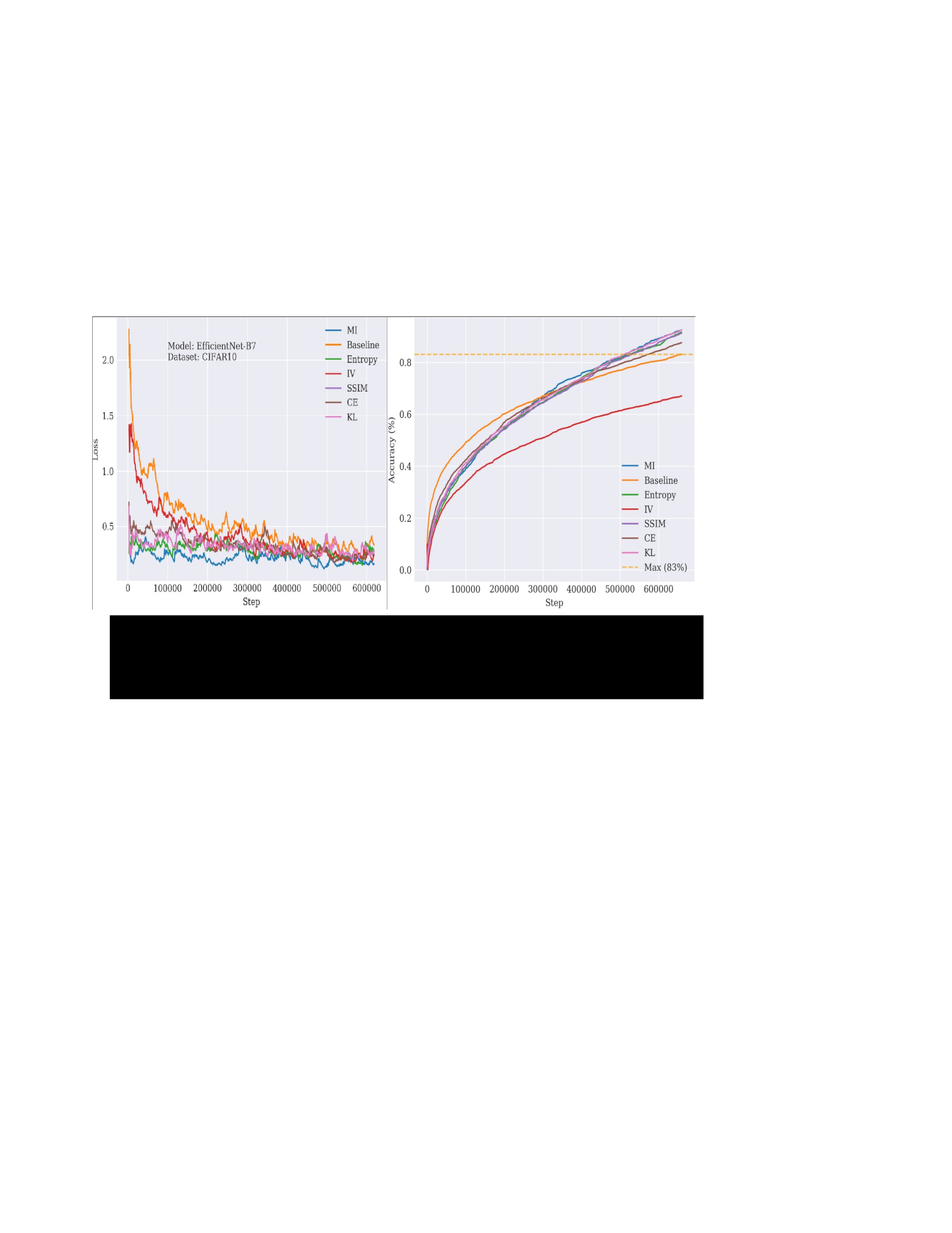
The architecture of the EfficientNet family is crafted to optimize performance and
efficiency, utilizing compound scaling on depth, width, and resolution of the model [140]. This
intrinsic efficiency is further amplified when paired with our curriculum learning strategies. Our
observations suggest that both EfficientNet-B7 and FixEfficientNet not only showcase enhanced
training performance but also demonstrate accelerated convergence. FixEfficientNet is
particularly notable in this regard. Its integration of newer weight update mechanisms, finetuning
resolutions during the training process, couples well with our curriculum learning
approach. This synergistic relationship allows the model to achieve performance benchmarks in
significantly fewer iterations, all the while maintaining its accuracy.
Validation Across Optimization Algorithms
Whilst these results are interesting, to rule out other factors of influence and ensure
repeatability across optimization algorithms, we whitelisted the best performing strategy in the
CIFAR10 experiment and performed similar experiments using ADAM and AdaGrad optimizers.
As depicted in Figure 5.12, when BiT-L was trained on CIFAR10, we observe a
consistent decline in training error. Most importantly, all the CL models not only managed to
rival the baseline's accuracy but achieved this feat with remarkable efficiency – typically
requiring up to
Figure 5.10. Left: Comparison of EfficientNet training performance on CIFAR10 and with and
without CLO (baseline). Right: Comparison of test performance of the same model under
different epochs on CIFAR10 held-out test set.
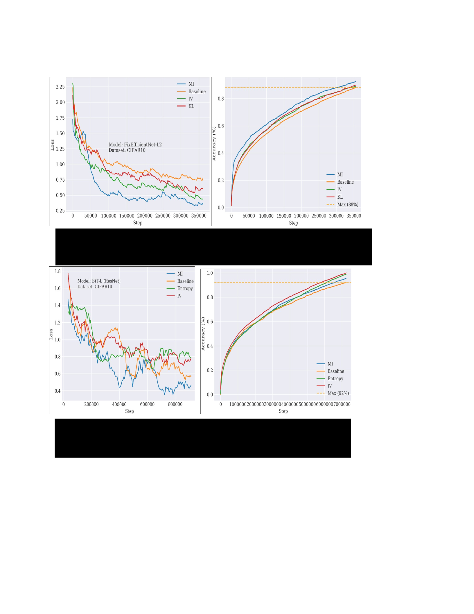
50,000 fewer iterations. Among the most compelling of these findings was the performance of
the IV-based syllabus. This strategy not only matched the maximum accuracy of the baseline,
which stands at 93%, but it did so in about 100,000 iterations fewer.
optimization landscape ADAgrad offers, especially its adaptive learning rate methodology, our
objective was to discern how our curriculum learning strategies hold up under its aegis. The
results are depicted in Figure 5.13. We observed a decline in training errors across the board yet
underscoring the efficacy of our approaches with the Mutual Information (MI) based syllabus
Figure 5.11. Left: Comparison of FixEfficentNet training Performance on CIFAR10 and with
and Without CLO (baseline). Right: Comparison of Test Performance of the Same Model on
CIFAR10 held-out test set.
Next, we trained ResNeXt on CIFAR10 using the ADAgrad optimizer. Given the unique
Figure 5.12. Left: Comparison of Bit-L Training Performance on CIFAR10 Using ADAM
Optimizer with And Without CLO (Baseline). Right: Comparison of Test Performance of the
Same Model Models on CIFAR10 Held-Out Test Set.

standing out. This strategy managed to reach the baseline's accuracy of 85% in just 1.3 million
iterations, as contrasted to the baseline's 1.75 million. Further, it pushed the envelope by
achieving an impressive 89% accuracy around the same 1.75 million iterations mark, indicating
not just faster convergence but also potential for enhanced generalization.
Validation Across Datasets
The test accuracy and training loss follow their usual course observed during CIFAR10
training when using CIFAR100 (Figure 5.14). The results on both datasets show that CL has
favorable impact on training performance. CL trained models achieve the same level of loss but
only require 2/3 of the steps compared to conventional training. These results also are in line with
the results on ImageNet presented in [23].
Results on Test Set
Another observation from this experiment is that most curriculum strategies produce
models that generalize better to unseen samples compared to the baseline (right column plots).
For instance, if we look at the test performance of Inception V2 trained using MI on CIFAR100
(Figure 5.14, right), the improvement on the test set is close to 15%. However, we also observe a
degradation in generalizability with some curriculum strategies. SSIM syllabus for instance is a
strategy that reduces generalization performance of ResNeXt-101 by 5% compared to the
baseline.
This is interesting, because it implies that the training improvements induced by the
proposed methods directly translate to performance gains in generalization for select networks.
This is beneficial because most models achieve similar accuracy as the baseline in significantly a
smaller number of iterations. Based on the experiments, VGG is the only model that does not
conform to these gains. The order of sample presentation in case of VGG may not be as
significant compared to the other architectures. We believe this is somewhat related to how the
model performs successive feature extraction in comparison to others.
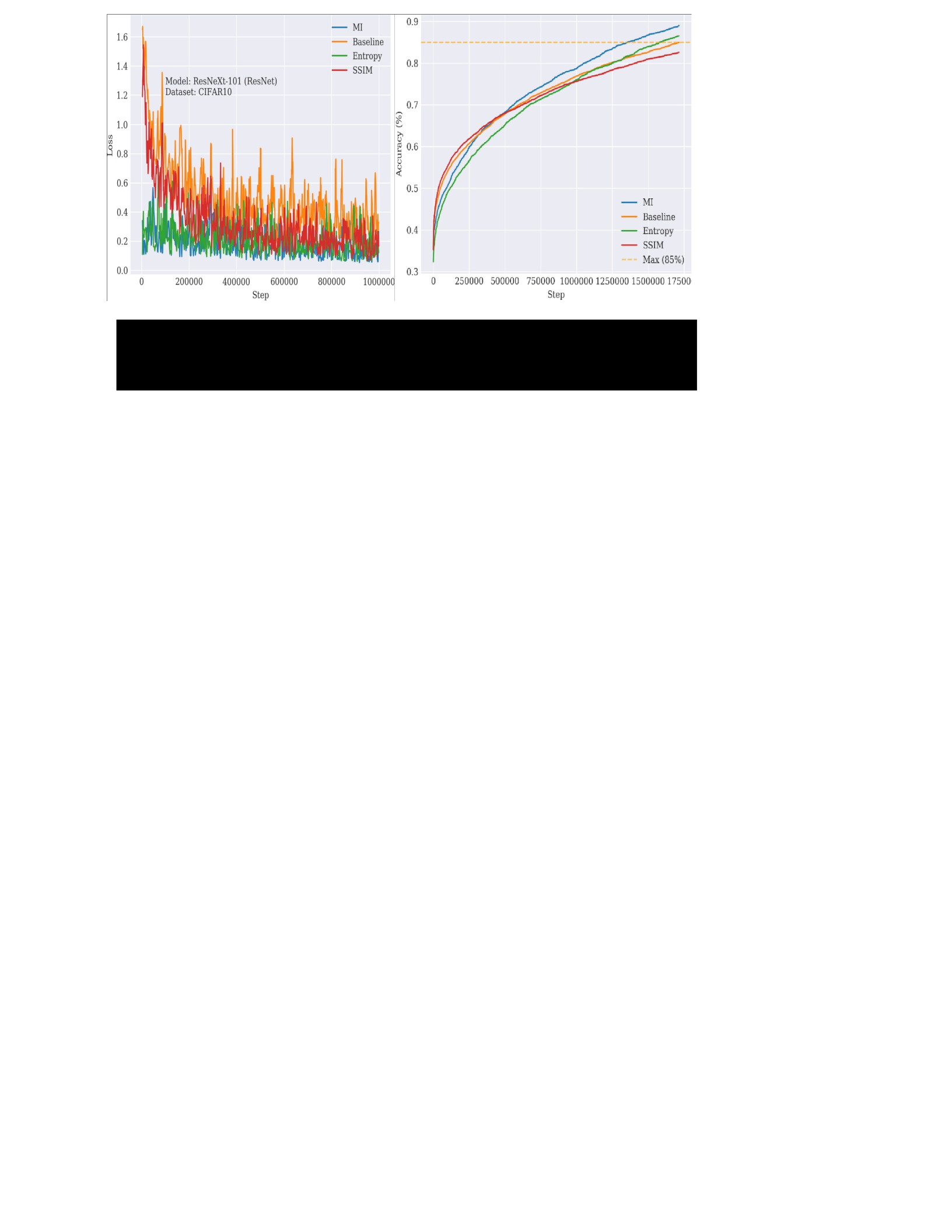
The results suggest that the curriculum learning technique that incorporates complexity of
training samples may be more effective not only in traversing the input space towards the ideal
minima but also has statistically significant impact on the classifier’s generalization performance
even when considering real-world scenarios (discussed below). Specifically, we see that the
variance in gradient direction of points (captured by the trends in loss) decrease much faster
when training using syllabus per batch in comparison to the traditional, random shuffling
approach.
Further Study on Generalization
When considering applicability of these models to real-world scenarios, the models must
go through validation process that considers variations and imbalance in real-world input. To this
end, we further assess generalization performance of models trained with the proposed method
using the CATS vs DOGS dataset for binary classification task. We choose binary classification
partly due to the rich and proven family of metrics for assessing applicability of classifiers to a
given domain. Taking sample complexity into account, in the context of curriculum learning,
may therefore increase the likelihood to achieve a higher quality local minimum during training
which in turn produces robust models with better generalization performance but in a smaller
Figure 5.13. Left: Comparison of ResNeXt Training Performance on CIFAR10 Using AdaGrad
and With and Without CLO (Baseline). Right: Comparison of Test Performance of the Same
Model Models on CIFAR10 Held-Out Test Set.

number of training iterations. The metrics, including the number of iterations, are presented in
column 3 of Table 5.2.
Table 5.2. Comparison of Generalization (Real-Time Inference) Capabilities of Various Models
with And Without Curriculum Learning. the Metrics That Outperform the Baseline Are
Highlighted in Bold.
Model Strategy # iterations
(10k)
p r F1-Score AUC Acc
(%)
ResNeXt-101 Baseline 19 0.54 0.55 0.54 0.74 0.63
ResNeXt-101-MI MI 15 0.67 0.73 0.70 0.81 0.78
VGG16 Baseline 6 0.83 0.85 0.84 0.89 0.91
VGG16-MI MI 6 0.86 0.75 0.80 0.82 0.84
BiT-ResNet Baseline 15 0.67 0.74 0.70 0.73 0.77
BiT-ResNet-MI MI 19 0.75 0.88 0.81 0.85 0.88
EfficientNet-B7 Baseline 8 0.58 0.53 0.55 0.992 0.88
EfficientNet-B7-MI MI 6.7 0.63 0.65 0.64 0.994 0.95
MobileNet V1 Baseline 6 0.88 0.88 0.88 0.992 0.88
MobileNet V1-MI MI 4.8 0.95 0.95 0.95 0.994 0.95
Inception v2 Baseline 6 0.94 0.95 0.94 0.94 0.93
Inception v2-MI MI 4.75 0.97 0.93 0.95 0.96 0.94
Figure 5.15 depicts the ROC curve of MobileNet performance on CATs vs DOGs using
various curriculum strategies. As can be seen in the plot, most CL strategies have AUC values
greater than the baseline. For instance, KL-syllabus trained MobileNet has an AUC value of
0.985 compared to 0.943 of the baselines. These values indicate that CL trained models have
to identify training strategies that expedite training, but also to produce more robust models for
practical applications.
Further Study on Optimization Methods

SGD and its variant Adam [79] work well for many optimization problems and can
converge to a promising local or global optimum within a reasonable computation cost. Instead
of computing loss on the whole dataset, SGD computes loss and weight updates on a batch of
samples and updates the model variables by computing the loss function gradient instances by
instances. SGD produces the same performance as regular gradient descent when the learning
rate is low. Another variant of gradient descent widely used in practice is Adam.
It is an adaptive learning rate method that combines the advantages of two SGD
extensions – Root Mean Squared Propagation (RMSProp) [88] and Adaptive Gradient Algorithm
(AdaGrad) [88]. It computes individual adaptive learning rates for different parameters of the
model. Unlike SGD, Adam updates exponentially moving averages of the gradients and the
square gradients whose decay rates are controlled by hyperparameters [79]. In this section of the
experiment, we use both optimization techniques to verify that our proposed method’s
performance is invariant to the type of technique used to update model parameters. The results
are depicted in Figure 5.16: Comparison of Adam and SGD Optimizers on Training Performance
of Inception Model When Trained Using MI CL Strategy..
The results show that the proposed method has comparable impact on training
performance when combined with SGD or Adam optimizer. In line with previous observations,
SGD progresses to find a minimum, but it takes significantly longer training time compared to
Adam. We observe a training loss reduction by factor of 1.75 when Deep-CLO is employed
alongside Adam, while the loss reduction with SGD is expedited by a factor of 1.8. The gap in
loss reduction as depicted in Figure 5.16 are inherent to the optimizers. This is because SGD is
much more reliant on a robust initialization and annealing schedule and may get stuck in saddle
points rather than local minima. So usually, SGD takes a greater number of iterations compared
to its variants. Adam on the other hand is an adaptive momentum and adaptive learning rate
algorithm which does not rely on robust initialization. Given these results, we hypothesize that

our proposed method is optimizer agnostic. In other words, the various CL strategies have
similar impact on training regardless of which optimizer is used.
In-Depth Analysis: Synergies between Curriculum Learning and Network Dynamics
In this section, we examine the interrelations between CL and core neural network
attributes, including regularization loss, sparsity, and strategy selection. Through some analysis,
we elaborate the influence of CL on these key aspects and its impact on overall network
performance and efficiency. The insights derived here shed light on the potential of integrated
approaches in enhancing model training.
CL Influence on Regularization Loss
As discussed in Chapter 2, regularization methods are supplementary techniques that are
used to reduce test error and prevent overfitting. These are reserved solely for a penalty term in
the loss function [29]. In all the networks used for this study, regularization is achieved by adding
a regularizer term 𝑙𝑟 to the native loss function. Unlike the loss function, which expresses the
deviation of the network output with labels, 𝑙𝑟 is independent of the labels. Instead, it is used to
encode other properties of the desired model to induce bias. These properties are rooted in
assumptions other than consistency of network output with labels. The most common approaches
are weight decay [152] and smoothness of the learned mapping. The regularization loss trends of
training various networks on CIFAR10 and CIFAR100 using JE and IV curriculum strategies are
depicted in Figure 5.17: Comparison of Regularization Loss of Several Curriculum Strategies
with the Baseline on CIFAR10 (Top) And CIFAR100 (Bottom).
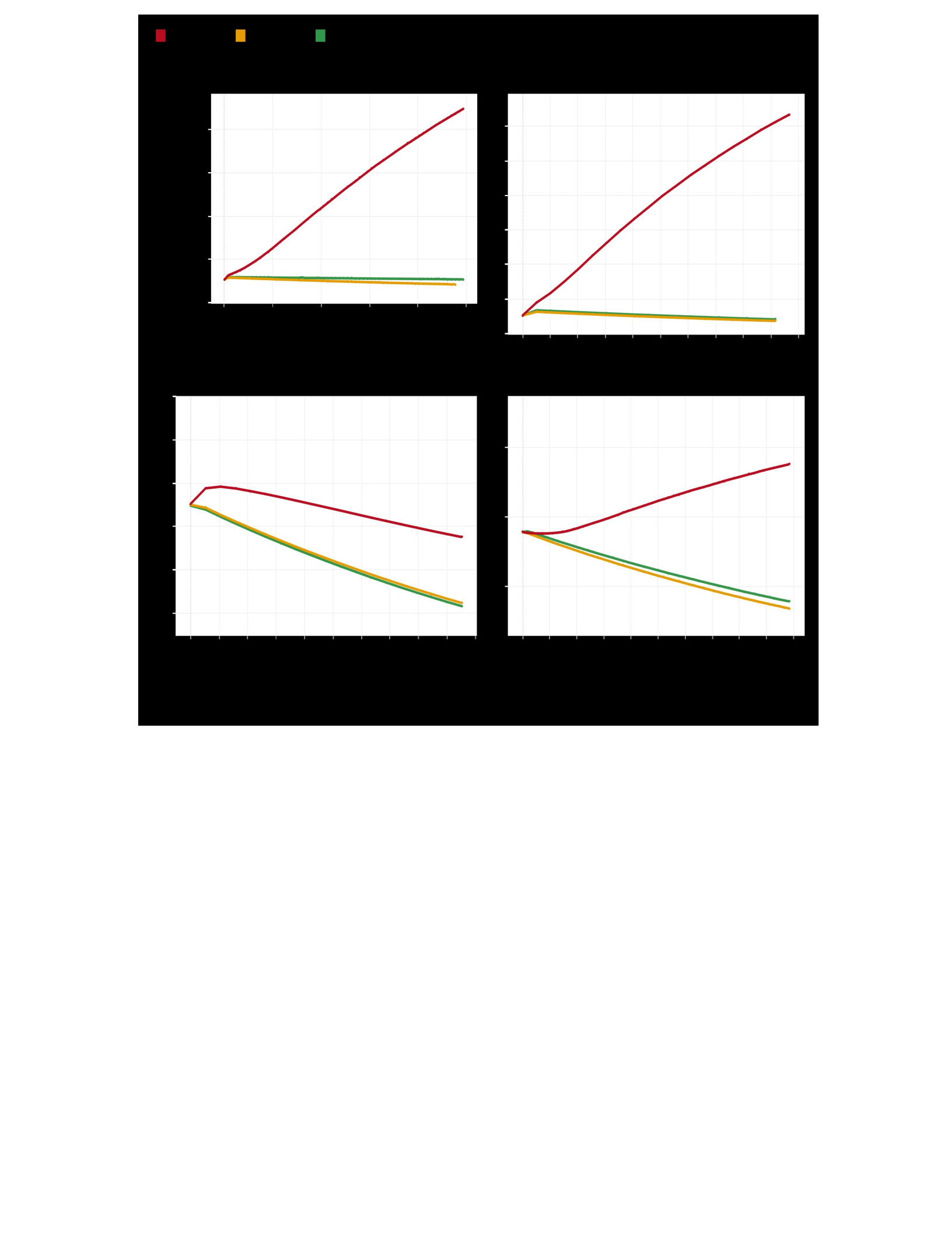
The plots reveal a distinction in the regularization loss trajectory when networks undergo
training on CIFAR10 and CIFAR100, specifically leveraging the JE and IV curriculum strategies.
It's evident that the regularizer term for the baseline encounters an abrupt escalation during the
initial 100K iterations, a trend contrasted when juxtaposed against our approach. This clear
demarcation underscores the palpable impact imparted by the CL method. Beyond serving as an
efficacious training strategy, CL intrinsically nurtures regularization within the model, obviating
the need for extended iterations with No-CL training to achieve this regularization.
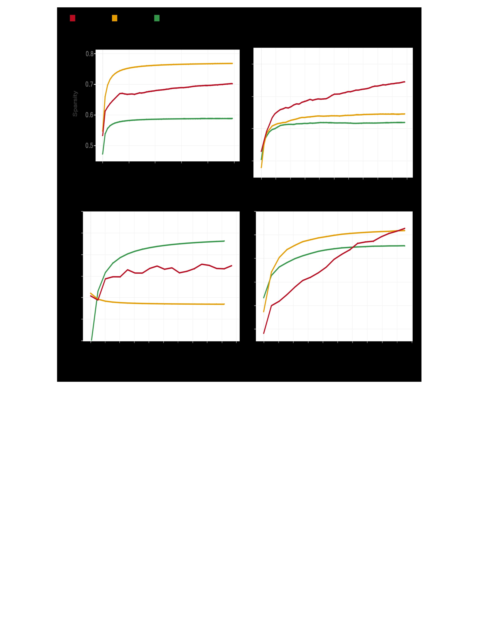
This intrinsic quality, we postulate, is instrumental in the accelerated convergence observed with
our models, accentuating the superior efficiency and potential of CL-driven approaches.
Sparsity
Output sparsity in deep neural networks is highly desirable to reduce model training and
inference costs. CNNs are highly sparse with many values involved in the calculations being zero
or close to zero. Features map sparsity can be exploited to expedite training and reduce inference
cost by skipping the values that are known to be zeros. Feature maps in CNN models usually
have high sparsity. This is because convolution operation is immediately followed by an
activation layer that turns all negative inputs into zeros. In addition, max-pooling layers only

select a max value in a sub-region of the input and drop other values in the region. As shown in
Figure 5.18: Sparsity Score of Select Layers of VGG16 (top) and Inception V1 (bottom) plotted
over a span of training iterations., we observe the average feature-map and fully connected layer
output sparsity scores are reduced much faster when training a network with the proposed
methods.
Selecting a Strategy
Most neural network-based machine learning algorithms come with millions of tunable
and user-specified parameters. Many of these parameters are encoded in the network architecture
and are tuned by the training procedure. In CNNs for instance, these types of parameters include
the convolution filter banks or weights which are tuned for a given dataset by the
backpropagation algorithm. While these are types of parameters that are automatically finetuned,
there also exist parameters such as learning rate and batch-size, commonly known as
hyperparameters, that are considered as tuning knobs of the learning system that researchers and
practitioners use to control the behavior of algorithm when optimizing its performance on a given
dataset. Hyperparameter tuning for performance optimization is a challenging problem and is a
subject of many machine learning researchers. As it currently stands, there are not established
rules for predicting the right set of parameters that guarantee best performance for a given
dataset [153]. Deep-CLO introduced one such hyperparameter, namely the metric (m), used to
construct a curriculum strategy. In this section we discuss our observation of one potential
approach to identify a strategy that is best suited for a given dataset. A more in-depth study
related to this is under way and will be considered in future publications.
Capturing Structural Information of Dataset
Figure 5.19 depicts the probability distribution of Entropy metric of the CIFAR10 and
100 datasets. The plots capture the distribution of the Entropy value of each sample as well as the
histogram of these values across classes (labels). We have found a strong correlation between the
extracted structural information of a dataset (such as distribution of Entropy) to the training and
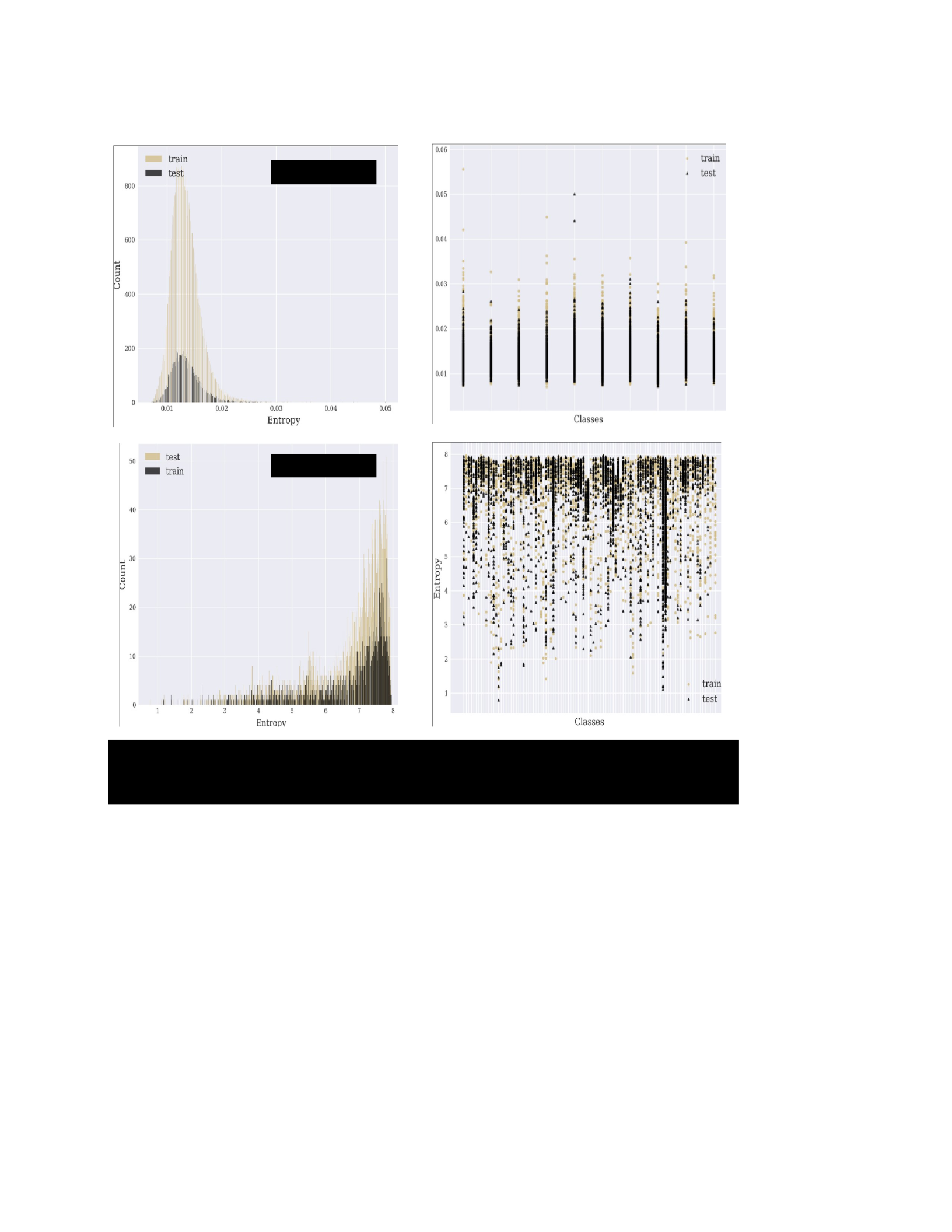
generalization trends of select models on that dataset. To illustrate consider the EfficientNet-B7
model performance (Figure 5.10) first column. The model achieves training loss of 0.3 when
trained using Entropy strategy on CIFAR10 dataset compared to 0.9 of the Baseline – a
statistically significant loss reduction which is induced by the proposed learning strategy. We
believe this performance optimization is somehow related to the structural information of the
dataset as captured by the metric. Entropy-based strategy favors such a reduction since Entropy
distribution (Figure 5.19, top) of CIFAR10 training set is a normal distribution with a mean of
0.1 and standard deviation of 0.0002. This structural information is also consistent with the test
set which enables us to predict the generalization gains of the strategy. The model trained with
Entropy strategy achieves similar accuracy as that of the Baseline in 3/4th of the number of
training steps. At the end, it beats the Baseline model by achieving 91% accuracy compared to
CIFAR100
Figure 5.19: Entropy Value Distribution (Left) and Distribution of Entropy Value Across Classes
for Both CIFAR10 (Top) And CIFAR100 (Bottom) Datasets.
CIFAR10

82%. On the other hand, performance degradation is observed when the same model is trained
using the same strategy on the CIFAR100 dataset. This observation we argue is predictable if one
sees the structural information of CIFAR100 as captured by the strategy in use (Figure 5.19,
bottom). The Entropy of every sample in CIFAR100 dataset significantly deviates from one
another’s by at least standard deviation of 2.6. In addition, Entropy value across the labels also
share such discrepancy making the strategy less effective at optimizing the model.
Although these kinds of characteristics are well suited to describing datasets, we believe,
when combined with the proposed training approach, they also enable us to recommend
appropriate classification models and strategy for a given dataset. Extracting and visualizing
structural information of the various metrics used in this study is relatively cumbersome and we
do not have a thought-out and efficient solution at this stage.
Summary and Conclusion
In this chapter, we delved deep into the application of the Deep-CLO framework,
introduced in the preceding chapter, specifically focusing on image classification. Through a
comparative study, we highlighted the merits and potential challenges of utilizing curriculum
learning in optimizing SOTA architectures over benchmark datasets. Our investigation distinctly
showcased significant training and generalization performance improvements when pitted
against the conventional, non-curriculum training.
By eliminating the need for manual sample ranking or multiple training passes, our
dynamic approach to proposing and evaluating the syllabus incorporated image analysis
techniques to seamlessly integrate into the deep learning-based training pipeline. It's noteworthy
that the adaptability of Deep-CLO means it remains independent of the model architecture,
allowing for individual component enhancement without any architectural modifications.
Our findings underscore the intricate relationship between sample ordering, the dataset in
question, and the chosen algorithm. A consistent observation was the reduction in loss during the
early training phases across all strategies, indicating the pronounced impact of our proposed

method. This effect was found to be independent of the optimizer but exhibited sensitivity to the
dataset. Notably, our experiments showcased that curriculum strategies often expedite the
training process without necessarily amplifying generalization performance compared to
traditional training.
The results suggest that while sample ordering does affect the training process, the
optimal order in which samples are presented may vary based on the dataset and algorithm used.
With all strategies, we found loss reduction at the initial stages of training to be the most
consistent signal that demonstrated the impact of the proposed method which is also optimizer
agnostic. However, it is sensitive to the type of dataset used for training. In addition to training
performance, we also notice improvements in generalization performance both in standard
testing scenarios and scenarios that consider real-world variations in input. The results indicate
that curriculum strategies reduce training loss faster without necessarily increasing the generalize
performance compared to conventional training. Our intuition is that the proposed technique
enables faster convergence by discovering optimal path that takes to local minima. However,
further analysis is required to fully test and prove our hypothesis that the proposed method
combined with gradient decent optimization expedites a search for local minima by creating an
optimal path in input space.

CHAPTER 6
APPLICATION OF PROSIS: ENHANCING CNN LEARNING THROUGH PATCH
REORDERING
Introduction
This chapter delves into the 2D reconstructed output of algorithm PROSIS, detailed in
Chapter 4 and highlighted in the publication Ghebrechristos et. al [20]. Our research is situated
within the broader landscape of CNN application in image classification tasks. A pivotal insight
anchoring our exploration is the innate capacity of CNNs to effectively train on datasets where
samples, to the human observer, appear devoid of any discernible correlation to their designated
labels. This uncovers a vital insight: the success of CNNs does not solely hinge on recognizable
human features.
At the heart of our methodology lies the concept of 2D reconstruction, as expressed by
Equation 4.32. Here, original samples undergo a transformation, wherein patches are
methodically positioned adjacent to each other. This sequence preservation from the ordered
patch list, 𝑅, crafts an image that maintains its original external dimensions but with internally
rearranged patch configurations.
This restructuring seeks to streamline feature extraction from images, making the most
out of CNNs' intrinsic capabilities. Drawing a parallel with CL, this algorithm offers an
interesting perspective. In CL, the learning process is guided by presenting samples in a
predetermined order. This aids in gradually training the model, with the premise being that
structured, gradual learning can lead to better and possibly faster convergence.

The subsequent sections of this chapter will detail the mechanics and rationale of
integrating PROSIS into deep learning pipeline, complemented by empirical evidence supporting
our claims.
Related Work
Given the context of our research, which centers around preprocessing image data using
patch reordering techniques, our literature review is specifically tailored to works that
manipulate or segment images into smaller units or patches. Of particular significance and the
only work related to ours is the Vision Transformers (ViTs) model, which underscores the
potential of treating images as sequences of patches [53]. Although this methodology was
introduced years after ours, it is worth examining its nuances and methodologies. In this section,
we delve into the details of the ViTs, outlining its objectives, technical specifics, results, and their
relationship with our approach.
Vision Transformers (ViTs)
Harnessing the power of the Transformer architecture [154], Vision Transformers were
conceptualized to leverage language processing mechanisms for image classification challenges.
By dividing images into a series of patches and subsequently processing them via Transformer
layers, ViTs aim to discern intricate inter-patch relationships, which might elude traditional
CNNs due to their localized receptive fields.
The approach can be encapsulated as a fusion of NLP and image classification
techniques. It hinges on the premise that, akin to the interrelation of words in a sentence, patches
within an image convey meaning through their interactions. By linearly embedding these patches
and subjecting them to Transformer layers, the model is positioned to perceive an image not just
as a single digital image, but as interconnected patches of images. ViT models consist of two key
components: patch embedding and positional encoding. Since Transformers were originally
designed for sequential data like text, where tokens (words or subwords) follow a clear order, but
images lack an inherent ordering of patches (small regions of the image) as seen in text. ViT

address this by dividing images into patches and treating each patch as a token; however, the
transformer architecture does not inherently understand the spatial arrangement of these patches,
requiring positional information to be added to capture the spatial structure effectively.
Like our approach, the foundational step is decomposing images into patches. Each image
is dissected into fixed-size, non-overlapping patches. These patches are subsequently flattened
and subjected to a linear transformation, rendering them as a set of vectors. This transformation
prepares the patches for the ensuing processing within the Transformer architecture. To safeguard
the spatial hierarchy of patches, Vision Transformers embed positional data into them. This
ensures that amidst transformations, the spatial narrative of the original image remains inviolate.
Performance Summary
Dosovitskiy et al. [53] presented comprehensive results of models ViT-H/14 and ViTL/16,
showcasing the transfer performance of ViT models pre-trained on datasets of varying sizes, from
ImageNet to JFT-300M [155]. These models segment images into fixed-size patches, linearly
embed them, and process them through transformer layers. The labels "H" and "L" denote model
sizes: "H" for huge models and "L" for smaller but large ones, while "/14" and "/16" specify
layer configurations. Their findings indicated that these models achieved competitive
performance on several benchmark datasets.
In the presented results both models consistently outperformed or closely matched the
performance of existing SOTA across various benchmarks. On ImageNet, ViT-H/14 achieved an
accuracy of 88.55%, slightly surpassing Noisy Student's [138] top performance of 88.4%. In the
CIFAR10 dataset, the ViT models showcased impressive results, with ViT-H/14 reaching
99.50% on CIFAR-10. For the broader VTAB assessment covering 19 tasks, ViT-H/14 led with
77.63%. Importantly, Vision Transformers demonstrated this superiority while consuming
significantly fewer computational resources, with ViT-H/14 and ViT-L/16 using just 2.5k and
0.68k TPUv3-core-days respectively, far less than the 9.9k and 12.3k of BiT-L and Noisy
Student.

Comparison with Our Approach
There are some parallels between our method and ViT’s approach. Both methodologies
underscore the significance of inter-patch relationships within an image. However, where our
approach seeks to optimize the sequence of input patches, ViTs focus on understanding their
interrelationships through the Transformer architecture. As our methodology was introduced
before the advent of ViTs, future research could explore potential synergies between the two.
Integration of PROSIS-2D into Deep Learning Training Pipeline
The process of constructing a training set for image classification tasks, especially in the
domain of supervised learning, requires a significant contribution from human labelers [63]. Let's
consider an example where the task is to classify images as either cat or dog. In such cases, the
human labeler needs to use their unique experience and judgment to categorize each sample
appropriately.
Such human involvement in the process presents a compelling question: Is human
classification performance on the training dataset critical to the learnability of the task? Could
CNNs still function with scrambled samples that might not be immediately distinguishable to the
human eye?
This was explored in depth in [15], where the researchers presented striking findings.
Despite traditional understanding, CNNs demonstrated the ability to fit a training set comprising
samples that were seemingly unrelated to their respective labels. These results posed a significant
challenge to the widely accepted belief that CNNs work by building a hierarchy of features in
increasing layers of abstraction. The traditional narrative suggests that the lower layers detect
basic features like edges, the middle ones recognize object parts, and the subsequent layers
identify complete objects.
Inspired by these revelations, we devise an approach to image preprocessing. If
humanrecognizable features are not a prerequisite for efficient CNNs, then our preprocessing
methods should focus on simplifying feature extraction for the network, not necessarily for the

human eye. This understanding forms the foundation of our strategy to integrate the PROSIS
algorithm into
CNN training pipeline.
Utilizing Algorithm PROSIS-2D for Feature Exposure
PROSIS-2D harnesses the intricate structures within images to facilitate more coherent
feature representations. As CNNs typically operate by learning features – both simple and
complex – the challenge often lies in ensuring that the essential features are accessible early in
the training process. These features are important in discerning the labels from one another.
Accessing them early during training can expedite convergence and potentially enhance
generalization. PROSIS-2D addresses this by emphasizing crucial features at the onset of
training.
As depicted in Figure 6.1 conventional CNN training involved a straight-forward
pipeline. The process typically begins with ingesting data, where a batch 𝐵 of raw images are
sampled from the dataset 𝐷. This is followed by an optional preprocessing phase, where each
image is subjected to operations such as resizing, normalization, and potential augmentations.
The process then proceeds to model training phase, where batches of the preprocessed images
are incrementally fed to the model, adjusting the model's weights and biases over time that
minimize prediction errors. The cycle concludes with an Evaluation phase, assessing the model's
performance against a validation dataset.
Instead of merely preprocessing the images, the goal of PROSIS-2D is to restructure the
image data in a way that is tailored to the architecture and nature of CNNs. Instead of providing
the model with raw or minimally processed images, PROSIS-2D ensures the images are
reordered to optimize feature accessibility, enhancing the model's capacity to detect and learn
from these features. CNN training pipeline that integrates PROSIS-2D is depicted in Figure 6.1.
The complete, end-to-end training algorithm is detailed in Algorithm 6.1.
Algorithm 6.1. PROSIS-2D Training of a Classification CNN Model G- .

Input: Ranking measure 𝑴, Training set D of size |𝐷|, Max number of training
steps 𝑵, Patch size 𝒘𝒑, 𝒉𝒑 ,Optional: Reference patch 𝑷𝒓𝒆𝒇
Output: Trained CNN model G-
1. Training Iteration:
oFor j from 1 to N:
§For each sample 𝒙𝒊 in 𝑻𝒔 :
§Draw a sample 𝒙𝒊.
§Generate patches set 𝑷 for 𝒙𝒊
§𝑷 ← {𝑷𝒊𝒋 ∣ 𝑷𝒊𝒋 = 𝒙[𝒊: 𝒊 + 𝒘𝒑, 𝒋: 𝒋 + 𝒉𝒑]}
2. Patch Processing and Ranking:
oFor each patch 𝒑𝒌 from 1 to 𝑷:
oIf 𝑴 is standalone:
§ Calculate the individual index for patch .
o Else:
§If 𝑷𝒓𝒆𝒇 isn't provided:
§Identify the patch with the minimal entropy and assign it as
𝑷𝒓𝒆𝒇
§Compute the similarity or distance index of relative to 𝑷𝒓𝒆𝒇.
3. Reordering and Reconstruction:
o Form the ranked patch list 𝑶
§ 𝒄 ← {𝒓𝟏, 𝒓𝟐,
… , 𝒓𝒁}
o Sort 𝑶
o Reconstruct image using reordered patches list 𝒙′𝒊
4. Training on Reordered Sample:
oTrain G- on the reordered sample 𝒙′𝒊
Return the trained model G-.

Experimental Setup
To evaluate this training strategy, we used CATS vs DOGS, CIFAR10 and 100 datasets –
described in Chapter 5. The preprocessing algorithm along with several network architectures
also discussed in Chapter 5, were employed to learn, and classify these datasets. To gather
enough data that enables characterization of each preprocessing technique, we set up a consistent
training environment with fixed network architectures, training procedures, as well as hyper
parameters configuration. The results are summarized in this section.
Results and Discussion
Impact on Training
Figure 6.2 shows results obtained when training Inception network to classify CIFAR100
(Top) and Cats vs Dogs (Bottom) datasets using slow learning rate and Adams optimization
[156]. Plots on the right side depict test performance of the network at different iterations. In
both setups, the mutual information technique speeds up the learning rate more than all others
while some techniques degrade the learning rate compared to regular training. However, all
techniques converge with the same performance as the regular training when trained for more
than 100000 iterations. Given these results we will answer the questions posed in the earlier
sections.
The question of whether ordering patches of the input based on some measure to help
training can partially be answered by the empirical evidence that indicates reconstructing the
input using the MI measure enables faster convergence. Dataset reordered using the MI measure
achieves similar accuracy as the unmodified dataset in ¼ of the total iterations. In support of this
we hypothesize that informed ordering techniques enable robust feature extraction and have the
potential to make learning efficient. To conclude, to prove this hypothesis, one must consider a
variety of experimental setups. For instance, to rule out other factors for the observed results, one
must perform similar experiments using different datasets, learning techniques, hyper parameter
configuration and network architecture.

Comparison with ViT
Table 6.1 below illustrates a side-by-side comparison of empirical results achieved by a
Baseline model, PROSIS-2D, and ViTs on several benchmark datasets.
For the CIFAR-10 dataset, the difference in performance among the models is narrow.
Yet, Vision Transformers, particularly ViT-H/14, slightly outpace others, although by a slim
margin. In the CIFAR-100 benchmark, PROSIS-2D remarkably surpasses the baseline model.
Interestingly, while ViT-L/16 demonstrates superb accuracy, ViT-H/14 lags, underscoring
that the architecture's size and configuration can influence performance across different datasets.
The distinction between PROSIS-2D and ViTs isn't merely numerical. PROSIS-2D places
emphasis on rearranging image patches in an optimal sequence to forefront pivotal features early
in training. This sequencing is tailored to bolster model convergence and potentially enhance
generalization. On the other end, ViTs, capitalizing on the capacities of Transformer architecture,
seeks to learn interrelationships between patches.
The PROSIS-2D's granular sequencing offers refined control over input representation,
which in theory, can facilitate better learnability. ViTs, contrarily, reinterpret the entire image
classification process, equating it to a language processing task.
While both methodologies emphasize dissecting images into patches, their core tenets and
strategies diverge profoundly. Empirical results, as illustrated above, highlight the distinct
strengths each brings to the table. Future exploration could pivot around combining these
strategies, potentially crafting an even more robust image classification paradigm.
Table 6.1. Comparison of Model Accuracies of Models Trained Using Our Approach Against
Vit.
Dataset Baseline Model/
Accuracy
PROSIS-2D ViT-H/14 ViT/16
CIFAR-10 EfficientNetV2-L/ 99.1 99.23 99.5 99.42
CIFAR-100 ResNeXt50/83.64 90.5 77.63 94.95

Analysis and Discussion
Given that most of these techniques remove human recognizable features by reordering
and the experimental results that not all ordering techniques compromise training or testing
accuracy, we make the following claim: Training and generalization performance of
classification networks based on the deep CNN architecture is uncorrelated with human’s ability
to separate the training set into the various classes.
Mutual Information in Image Patch Ordering
In this section we provide pseudo-analysis to corroborate the above claim. Let us consider
the mutual information (I) metric, which outperforms all other metrics. As mentioned in previous
sections the MI index is used as a measure of statistical dependency between patches for patch
ordering. Given two patches 𝑝4, 𝑝R, the mutual information formula (Eq. 10) computes an index
that describes how well you can predict 𝑝R given the pixel values in 𝑝4. This measures the
amount of information that image 𝑝4 contains about 𝑝R. When this index is used to order patches
of an input, the result consists of patches ordered in descending order according to their MI
index. For instance, consider a 32 by 32 wide image with sixteen 8 by 8 patches (see
representation, I, below). If we take patch 𝑝(0,0) to be the reference patch, Algorithm 2 in the
first iteration computes MI index of every other patch with the reference patch and moves the
one with the highest index to position (0,1) and updates the reference patch. At the end, the
algorithm generates an image such that the patch at (0,0) has more similarity to patch at (0,1)
which has more similarity to patch at (0,2) etc. In other words, adjacent patches explain each
other well more than patches that are further away from each other. How does this impact
training?
Consider the convolution operator [157] and the gradient decent optimization [158]
approach. This algorithm employs Adam optimization technique and SoftMax cross-entropy loss,
to update network parameters. Assume an online training [130] mechanism, where error
calculations and weight updates occur for every sample. Our hypothesis is that samples

preprocessed using the MI measure enable rapid progress lowering the cost in the initial stages
of the training. In other words, when the input is rearranged such that adjacent samples have
similar pixel value distribution, the convolution filters extract features that produce smaller
errors. To illustrate this let us assume the following values for the first few patches of an image
(color coded in the matrix below). For simplicity let us assume the image is binary and all the
pixel values are either 0 or 1.
0 0 0 0 0 1
⎡⎢0 0 1 1⎤⎥
𝐼𝑚= ⎢⎢101010 10⎥⎥
⎢0 0 1 0⎥
⎣1 0 0 1⎦
Also consider the following 3x3 convolution filter whose values are initialized
randomly: 𝐾 =
Ø1 5Œ. If one performs convolution of the original image with the above kernel 𝐾, the
resulting 0 1
feature map consists of the following values.
0 0 0 0 0 1
⎡0 0 1 6 6 6⎤⎥
⎢
𝐼𝑚 ∗ 𝐾 = ⎢10616171 7171⎥⎥
⎢
⎢0 0 1 0 0 1⎥
⎣1 0 0 1 1 0⎦
To maintain resolution of the original image we use 0-padding before applying
convolution. Applying a 3x3 max pooling operation with stride 3 to the convolved sample
generates a down-sampled feature-map of the 𝑖&: training sample 𝑥9 = Ø6171Œ which
is used as an input to compute probability score of each class in a classifier. In this illustration we
consider a binary classifier with two possible outcomes.
1 1
1 1
0 0
0
11
0

Given a weight matrix 𝑾 = Ø0.01 −0.05 0.1 0.05Œ and a bias vector 𝒃 =
Ø 0.2 Œ, 0.7 0.2 0.05 0.16 −0.4
the effective SoftMax Cross-Entropy loss (Equation 2.14) for the correct class can be computed
using the normalized probabilities assigned to the correct label 𝒚𝒊 given the image 𝒙𝒊
parameterized by 𝑾.
The probabilities of each class using Equation 2.9 objective function, after normalization is
Ø0.01Œ. Assuming the probability of the correct class is 0.01 the cross-entropy loss becomes
4.60.
0.99
Note here patches are ordered from left to right and adjacent patches have MI indices that
are larger than those that are not adjacent. After ranking each 3x3 patch using the MI measure
and preprocessing the sample using Algorithm PROSIS-2D, the resulting sample 𝐼′ has ordering
grey, green, pink, and blue. In this example MI of the green with the grey patch is 0.557 while
the blue has MI index equal to 0.224 against the same reference patch.
0 0 0 0 0 0
⎡⎢0⎤⎥
𝐼𝑚′ = ⎢⎢10⎥⎥
⎢0⎥
⎣1⎦
Once 𝐼𝑚′ is convolved using the same kernel 𝐾, the resulting downscaled feature
map, 𝒙𝒊G =
Ø6 5Œ, produces Ø0.13Œ probabilities for each class. Taking the negative
logarithm of the 6 7 0.87
correct class results in a prediction loss equal to 2.01.
This is the underlying effect we would like all measures to have when reordering the
training dataset. However, it is not guaranteed. For instance, if we use l2-norm measure (Eqn. 12)
to sort the patches, the resulting loss becomes 4.71, which is higher compared to the unmodified
0 0 1
1 1 0
0 0 1
1 1 1
1 1 1
0 1
1 1
0 0
0 1
0 0

sample. As a result, the training is slowed down since larger loss means more iterations are
required for the iterative optimization to converge.
Patch Size Impact on Training
To characterize the effect of patch size, we performed controlled experiments where only the
patch size is the varying parameter. The results and unmodified and preprocessed samples are
depicted in Figure 6.3. Comparison of Training Performance of Inception Using Different Patch
Sizes. CIFAR10 (Left) and CIFAR100 (Right) Datasets. Total Training Loss (Top) and
Regularization Loss (Bottom) for Unmodified Dataset, and Datasets Modified by Applying
Algorithm 6.1 Using the MI Metric and Patch Sizes 4 × 4, 8 ×8 and 16 × 16).
The Overall Size of Each Sample is 32 × 32.
As can clearly be seen in the plot, the network makes rapid progress, lowering the cost
when trained on a 4x4 patch ordered dataset. Based on empirical evidence and observations, we
believe patch-ordering impact is more effective when mutual information index is combined with
small patch size. To clarify consider dividing the above sample into nine 2x2 patches.
0 0 0 0 0 1
⎡⎢0 0 1 1 1 1⎤⎥
𝐼′′ = ⎢1 1 1 1 1 1⎥
⎢0 0 0 0 0 0⎥
⎢0 0 1 0 0 1⎥
⎣1 0 0 1 1 0⎦
normalized prediction probabilities are Ø0.14Œ, which results in a loss of 1.96 after the first
0.86
iteration.
This is one explanation for the observed results; however, we cannot draw any
conclusions regarding proportionality of patch size to training performance. If the pink and red
patches of the above sample, which have the same MI index, were to swap places, the resulting
loss would have been 4.71 which is greater than the loss generated using 3x3 patch size. In this
scenario training is slowed down.

Advantages and Implications of PROSIS-2D Integration with Human Labeling
Perspective
When we consider the traditional methods of constructing training sets, especially for
supervised learning tasks in image classification, the role of human involvement is paramount.
This involvement isn't just about label assignment; it's also about the inherent human
understanding of the features within images. However, as we step into the realm of machine
learning, especially with tools as powerful as CNNs, it begs the question: To what extent is the
human perceptual understanding of features crucial for a machine's learning?
When a human labeler designates a picture as, say, a "cat" or a "dog," they're doing so
based on their understanding and recognition of features, patterns, and nuances within the image.
These nuances, which are clear and evident to a human eye, drive the label assignment. CNNs
operate differently. They prioritize features differently, often in ways not immediately intuitive to
human perception.
By reordering and restructuring the images to accentuate these machine-centric features,
PROSIS-2D can expedite training and improve generalization. Allowing CNN to focus on a
version of the dataset where features are most pronounced – even if these are not what humans
would typically note – might give the model a more nuanced grasp of the data.
Balancing Human and Machine Perspectives: Implications
So, to what extent is human perception crucial? While the advantages of PROSIS-2D are
promising, it's vital to recognize the implications. There's an intrinsic value in human cognition
and the way we understand and interpret visual data. Completely sidelining this perspective
might mean missing out on certain nuances that only human cognition can capture. Therefore,
while machines might not necessarily need data in the exact format that humans understand it,
there's still merit in considering the human perspective, especially in the initial phases of data
labeling.

Conclusion
The integration of PROSIS-2D into the training pipeline offers a renewed perspective on
the dynamic between human cognition and machine learning. While machines like CNNs might
not necessarily require human-readable data structures, the underlying features – both humans
and machines recognize for classification– remain crucial. The task at hand is to find the optimal
point where human understanding and machine efficiency intersect, ensuring both speedy and
robust model training.
CHAPTER 7
APPLICATION OF PROSIS-3D: ENHANCING CNN SECURITY THROUGH
VOLUMIZATION AND 3D CONVOLUTION
Introduction
In the realm of machine learning, the security of models is predominantly gauged by their
resilience to adversarial attacks [159]. These attacks employ meticulously crafted perturbations,
often barely perceptible, which, when introduced to the input, can lead to misleading model
predictions. Classified into black-box or white-box attacks based on the attacker's knowledge and
access to model details, these techniques represent significant threats to model integrity [160].

In white-box attacks [161], attackers operate with comprehensive knowledge of the
model, from its architecture to its trained parameters. In stark contrast, black-box attackers
operate with limited insight, relying on observed outputs for given inputs [162]. A middle
ground, termed the gray-box attack [163], utilizes generative models to craft adversarial inputs
without specific knowledge of the victim model.
A particularly potent subset of these attacks is the localized adversarial attacks [164].
Capitalizing on the spatial invariance property of CNNs, these attacks introduce minimal but
strategically placed perturbations, causing the models to misclassify.
This chapter delves into the application of PROSIS-3D in enhancing the robustness of
CNNs against localized universal pixel perturbations. By universal we mean these are black-box
attacks that affect any pretrained model. In combination with deep curriculum optimization,
PROSIS-3D leverages input volumization to proactively defend localized universal attacks. The
method synergizes batch-based CL, patch aggregate loss (PAL) function, and 3D convolution to
proactively shield models.
Key contributions of this chapter include:
•Introduction of a groundbreaking training strategy combines PROSIS-3D with deep
curriculum learning optimization and 3D convolution.
•Empirical demonstrations establishing the efficacy of this strategy, underscoring its potential
in crafting models that stand resilient against localized attacks, ensuring robust generalization
and fortified defenses against adversarial attacks.
Background on Adversary Attack
At its core, the purpose of adversary attack is to sabotage the generalization capability of
a model by countering its learning objective. Given a CNN classifier 𝑓(𝑥; 𝜃), fully
trained on a dataset 𝐷 (Equation 2.9), its purpose is to map a source image 𝑥 to a set of
probabilities 𝑓(𝑥). An adversarial attack seeks to perturb this source image, producing an altered
image 𝑥′ such that the difference between 𝑥 and 𝑥′ is minimal to human perception. However,
the classifier 𝑓, when processing 𝑥′, produces an incorrect output that significantly deviates
from the true label. This is achieved by exploiting the high-dimensional decision boundaries of
the model, forcing it to misclassify 𝑥′ while maintaining a semblance of the original image
structure in 𝑥.
Attack Objective
Adversarial image attacks involve adding a perturbation 𝑟 to 𝑥 , causing the
maximized class probabilities to differ between the original and perturbed images. i.e.,
𝑎𝑟𝑔𝑚𝑎𝑥9(𝑓9(𝑥 + 𝑟) ≠ 𝑎𝑟𝑔𝑚𝑎𝑥9(𝑓9(𝑥)). These types of attacks can be categorized as
targeted or untargeted.
In a targeted attack, the adversarial image 𝑥′ = 𝑥 + 𝑟 is generated to induce the classifier
to assign 𝑥′ to a specific target class 𝑐& ∈ Y, where 𝑐& ≠ 𝑎𝑟𝑔𝑚𝑎𝑥9(𝑓9(𝑥)). The
perturbation 𝑟 is selected such that 𝑎𝑟𝑔𝑚𝑎𝑥9(𝑓9(𝑥′)) = 𝑐&. Conversely, in an
untargeted attack, the adversarial image 𝑥′ = 𝑥 + 𝑟 is crafted to cause the
classifier to assign 𝑥′ to any incorrect class without a particular target. In this case, the
perturbation 𝑟 is chosen to satisfy 𝑎𝑟𝑔𝑚𝑎𝑥
𝑎𝑟𝑔𝑚𝑎𝑥9(𝑓9(𝑥)) without imposing additional constraints on the target class. Our
research focus is untargeted attacks.
Defense Objective
The defense objective is to train a model that is robust to adversarial image attacks
without sacrificing the accuracy of the classifier on the original dataset. Formally, the objective is
to find 𝑔 that minimizes the following loss:
𝑚𝑖𝑛q|
(7.1)
4
+|∑𝑚𝑎𝑥
[ ∈r �
�
(𝑔(�
�
+𝑟),�
�
)
(C,O)∈+

where 𝑅 is the set of possible adversary perturbations added to a local region of the input, and 𝐿
is a loss function used to train the model 𝑔. The objective is to minimize the maximum loss over
all possible adversarial examples 𝑥′ = 𝑥 + 𝑟 generated by any allowable
perturbation in 𝑅. 𝑅 is constrained to be a set of localized attacks. Localized attacks are
characterized by the property that the L2 norm of the perturbation vector 𝑟, denoted by ||𝑟||, is
much smaller than the L2 norm of the original input image 𝑥, denoted by ||x||. Specifically, this
condition can be expressed as ||r|| << ||x||. These attacks modify only a small subset of pixels that
are confined to a localized region of the image.
Localized Universal Attacks Against Image Classifiers
Localized universal attacks are a subset of adversarial attacks that specifically target
image classifiers. They exploit spatial invariances of Convolutional Neural Networks (CNNs) to
introduce perturbations that lead to misclassifications. These perturbations are usually confined
to small, contiguous portions of the input image and can cause the model to produce incorrect
output classifications, even when the introduced changes are almost imperceptible to the human
eye. Two predominant types of such attacks are the N-Pixel Attack and the Adversary Patch
Attack.
N-Pixel Attack
Szegedy et al. introduced adversarial attacks through minor perturbations of pixels [15] to
induce CNN image misclassification. These perturbations, often undetectable to the human eye
(see Figure 7.1), expose the inherent vulnerabilities in the robustness of Convolutional Neural
Networks (CNNs).
Diving deeper into this, the N-Pixel Attack, which can be viewed as an extension or
generalization of the ideas presented by Szegedy et al., specifically perturbs 'N' distinct pixels in

an image to induce misclassification. The challenge and intrigue of this method arise from its
seemingly benign nature; altering a minimal number of pixels in a high-resolution image
intuitively appears harmless. Yet, such alterations can drastically alter CNN’s prediction,
underscoring the intricate and potentially fragile decision boundaries upon which these networks
operate.
While the attack has profound implications for the integrity and reliability of image
classifiers, it also catalyzes a renewed interest in understanding the foundational workings of
CNNs. This understanding is crucial, especially in applications where trust in model predictions
is paramount, such as in medical imaging or autonomous vehicles.
The N-Pixel Attack serves as a pivotal reminder that even state-of-the-art models, trained
on extensive datasets and exhibiting high accuracy, can be vulnerable to carefully constructed,
minimal adversarial perturbations. As researchers and practitioners continue to deploy CNNs in
varied applications, it is imperative to develop strategies that not only enhance performance but
also fortify against adversarial threats.
Adversary Patch Attack
Introduced by Brown et al., the Adversary Patch Attack unveils a unique and potent
vulnerability in deep neural network (DNN) based classifiers [165]. Unlike other adversarial
attacks that perturb an image globally, this approach is localized and focuses on modifying a
confined region of the image with an adversarial patch, which can be recognized as a seemingly
harmless object or pattern added to the image. Remarkably, this addition can dramatically alter
the classifier's output, demonstrating a classifier's inability to discern genuine content from
deceptive information.
Central to the findings of Brown et al. was the realization that these adversarial patches
were resistant to various changes, especially affine transformations such as translation, scaling,
and rotation. Their methodology optimized the patches such that they were robust to these
transformations. This means that the relative position, size, or orientation of the adversarial patch

doesn't need to be precise for it to deceive the classifier effectively. This robustness elevates the
potential real-world implications of this attack as the adversarial patch remains effective under
different viewing conditions.
The adversarial patch, crafted using a white-box approach, can be applied in a "universal"
manner. This universality signifies that a single patch can be effective across different images
and is not tied to a specific target image. The conspicuous nature of these patches (often visually
distinct) contrasts with the often-imperceptible alterations in traditional adversarial attacks,
making it an intriguing anomaly in adversarial research.
Furthermore, Brown et al.'s findings underscore the importance of understanding not just
the global, but also the localized processing dynamics of CNNs. The attack challenges the
prevalent notion of CNNs' spatial hierarchies, wherein larger spatial structures (like objects) are
assumed to have a dominant influence over classification compared to smaller structures or
patterns. The Adversary Patch Attack highlights that this might not always be the case, as a
localized, conspicuous pattern can effectively override the neural network's perception of larger
structures.
In real-world scenarios, this type of attack could be employed in deceptive practices, such
as placing adversarial stickers or objects in strategic locations to deceive AI systems in
surveillance, autonomous driving, or even augmented reality applications. As such, the research
by Brown et al. underscores the importance of defensive mechanisms that consider both global
and local image features.
Both Brown et al., and later Gittings et al. [166] backpropagate through the target model
to generate ‘stickers’ that can be placed anywhere within the image to create a successful attack.
This optimization process can take several minutes for one single patch. Karmon et al. showed in
LaVAN that the patches can be much smaller if robustness to affine transformation is not
required [164] but require pixel-perfect positioning of the patch which is impractical for real
APAs.

Related Work
Goodfellow et al. proposed a method to enhance the robustness of neural networks
against such attacks. This approach, known as adversarial training [167], involves using
adversarial examples as inputs during training to teach the network how to accurately classify
them, thus improving its ability to defend against attacks. Adversary training methods require
access to the target model to backpropagate gradients to update pixels, inducing high frequency
noise that is fragile to resampling. In 2016 Papernot et al. proposed a defensive mechanism
called defensive distillation [168], in which a smaller neural network learns and predicts the class
probabilities generated by the original neural network’s output. Despite growing number of
defense approaches, several attacks remain effective – particularly attacks generated using
generative architectures [169], [170].
N-Pixel Attack Defenses
Brown et al. demonstrated that adversarial patches could be used to fool classifiers; they
restricted the perturbation to a small region of the image and explicitly optimized for robustness
to affine transformations [165]. Su et al. in 2017, which generates fooling images (adversarial
examples) by perturbing only one pixel or few pixels, has proven to be difficult to defend [171].
To date, the most successful defense against this attack is a method presented by Chen et al.
[172]. The authors propose Patch Selection Denoiser (PSD) that removes a few of the potentially
attacked pixels in the whole image. At the cost of image degradation, the authors achieve a
successful defense rate of 98.6% against one-pixel attacks. Similarly, Liu et al. [173] proposed a
three-step image reconstruction algorithm to remove attacked pixels. The authors report
protection rate (defense success rate) of up to 92% under for N-pixel attack for N chosen from
the range (1, 15). Shah et al. [174] proposed the usage of an Adversarial Detection Network
(ANNet) for detection of N-pixel attacks where N is 1, 3 or 5 and report up to 97.7 adversarial
detection accuracy on MNIST Fashion dataset. Husnoo and Anwar [175] proposed an image

recovery algorithm based on Accelerated Proximal Gradient (APG) [176] approach to detect and
recovered the attacked pixels.
Adversary Patch Defenses
Defenses for patch attacks are typically viewed as a detection problem [177], [178]. Once
the patch’s location is detected, the suspected region would be either masked or in-painted to
mitigate the adversarial influence on the image. Hayes [179] first proposed DW (Digital
Watermarking), a defense against adversarial patches for nonblind and blind image inpainting,
inspired by the procedure of digital watermarking removal. A saliency map of the image was
constructed to help remove small holes and mask the adversarial image, blocking adversarial
perturbations. This was an empirical defense with no guarantee against adaptive adversaries.
Naseer et al. [180] proposed LGS (Local Gradient Smoothing) to suppress highly activated and
perturbed regions in the image without affecting salient objects. Specifically, the irregular
gradients were regularized in the image before being passed to a deep neural network (DNN)
model for inference. LGS could achieve robustness with a minimal drop in clean accuracy
because it was based on local region processing in contrast to the global processing on the whole
image as done by its counterparts. Chou et al. [181] proposed SentiNet for localized universal
attacks to use the particular behavior of adversarial misclassification to detect an attack, which
was the first architecture that did not require prior knowledge of trained models or adversarial
patches. Salient regions were used to help observe the model’s behavior. SentiNet was
demonstrated to be empirically robust and effective even in real-world scenarios. However, it
evaluated adversarial regions by subtracting the suspicious region, which might at times cause
false adversarial region proposals. Moreover, the suspicious adversarial region was placed at
random locations in the preserving image, which possibly occluded the main objects in the scene
resulting in incorrect predictions. Chen et al. [182] proposed Jujutsu to detect and mitigate
robust and universal adversarial patch attacks by leveraging the attacks’ localized nature via
image inpainting. A modified saliency map [183] was used to detect the presence of highly active

perturbed regions, which helped to place suspicious extracted regions in the least salient regions
of the preserved image and avoid occlusion with main objects in the image. Jujutsu showed a
better performance than other empirical defenses in terms of both robust accuracy and low false-
positive rate (FPR), across datasets, patches of various shapes, and attacks that targeted different
classes.
Instead of relying on patch or pixel detection and removal techniques, our method uses
deep curriculum learning optimization (Deep-CLO) [184] and 3D convolutional neural networks
[185] to proactively defend against these attacks. An overview of our proposed training
methodology is depicted in Figure 7.3.
PROSIS-3D Integration
Our aim is to develop a defended classifier,G-, that inherently defends against localized
attacks without relying on adversarial training or prior knowledge of the attacks. To achieve this
objective, we propose a proactive defense approach characterized by the following key steps:
•Volumization: For each image in the batch, we convert it to a 3D volume to capture the
spatial information of the input.
•3D Convolution: We modify contemporary CNN model architectures to do 3D convolution,
which enables the model to extract features from the 3D input volumes. Details of the
modifications are below.
•Deep curriculum learning optimization: For each batch taken from the training dataset D, we
generate a syllabus that determines the input order of the samples in the batch.
The combination of 3D convolution, Deep-CLO, and the volumization algorithm
empowers G- to maintain high performance on both clean and adversarial inputs. These
techniques ensure that the model remains resilient to perturbations and that it maintains accurate
classification and verification of both the original images 𝑥 and adversarial images 𝑥′ =
𝑥 + 𝑟. Refer to the analysis section for detailed justification.
When used as a preprocessing step, the algorithm allows G- to extract spatial relationships
from the volumized data, resulting in enhanced robustness against localized attacks. The
employment of Deep Curriculum Optimization as the training procedure further bolsters the G-’s
resilience to adversarial attacks. The resulting classifier not only defends against the targeted
attacks but also retains high performance on non-adversarial images, achieving classification
accuracy comparable to state-of-the-art models. Consequently, our approach demonstrates a
unique balance between robustness and accuracy without relying on adversarial training, making
it a significant contribution to the field of image classification under adversarial conditions.
Model Architecture
Given a conventional CNN classifier architecture 𝑓designed to learn from 2D
images, we perform the following modifications to construct G- - a 3D counterpart 𝑓.
Input layer
𝑓’s input layer, denoted as 𝐼R+, is designed to accept a 2D input data 𝑥with
dimensions 𝐻 × 𝑊 × C such that 𝐼R,×/×1. In order to extract features from the
volumized images, the input layer of model G- is adjusted to be 3-dimensional, 𝐼a+, where the
input to this layer 𝑥( is a 4D tensor with dimensions 𝐻′ × 𝑊′ × C × Z, such that 𝐼a+: 𝑥( ∈
ℝ,G×/G×1×0. In shorthand notation, this reversible transformation can be represented as:
𝑓,×/×1) ↔ G- ,
(7. 2)
where 𝐻’ and 𝑊’ are prespecified width and height of the individual patches within the
volume and 𝑍 signifies the total number of patches. This enables the classifier to learn features
from the volumized data 𝑥(.
3D Convolution
For CNN, convolution represents the interaction between an input (image or feature map)
and a kernel (filter). The kernel is a small matrix that slides over the input data, performing an

element-wise multiplication and summing the results to generate a new feature map. In a 2D
convolution, the input data and the kernel are both two-dimensional. (𝐾 ∗ 𝑥)(𝑖, 𝑗) = ‘‘ 𝐾(𝑚,
𝑛)𝑥(𝑖 − 𝑚, 𝑗 − 𝑛)
(7. 3)
8 %
Here, 𝐾 represents the 2D kernel, 𝑥 represents the 2D input and (𝑖, 𝑗) are the coordinates in the
output feature map. The summation is performed over all spatial dimensions (𝑚, 𝑛) of the 2D
kernel.
For a given classifier, 3D counterpart of the above operation is: (𝐾a+ ∗ 𝑥()(𝑖, 𝑗, 𝑘) =
‘ ‘ ‘ 𝐾a+(𝑚, 𝑛, 𝑝)𝑥((𝑖 − 𝑚, 𝑗 − 𝑛, 𝑘 − 𝑝)
(7. 4)
8 % ‘
where 𝐾a+represents the 3D kernel, 𝑥( is the 3D input data and (𝑖, 𝑗, 𝑘) are the coordinates in
the output feature map. The summation is performed over all spatial dimensions (𝑚, 𝑛, 𝑝) of
the 3D kernel. This modification enables the classifier to learn features from the volumized data
by processing spatial information across height, width, and depth dimensions simultaneously.
Note that the optimal kernel size depends on the size of the individual slices within the
volume and the desired level of spatial information capture. For example, if f consists of 1 × 1,
3 × 3, and 5 × 5 2D convolution layers, we adjust these layers to be 1 × 1 × 𝑍, 3 × 3 × 𝑍,
and 5 × 5 × 𝑍 3D convolution layers, respectively. To ensure compatibility, we enforce the
constraint that the kernel size is much smaller than the size of the individual slices and that the
kernel operates on each slice in the volume. That is, 𝐻′ ≪ 𝐻, and 𝑊′ ≪ 𝑊. The
stride and padding values are also adjusted accordingly.
Pooling Layer

All pooling layers of 𝑓 are modified to handle the 3D volume representation of the input
data. In 𝑓, the 2D pooling layers denoted as 𝑃R+:
𝑃R+: ℝ,&(×/&(×1&( → ℝ,234×/234×1234 (7. 5)
where 𝐻9%, 𝑊9% and 𝐶9% represent the height, width, and number of channels of the
input feature maps, while 𝐻Is&, 𝑊Is& and 𝐶Is& denote the height, width, and number of
channels of the output feature maps, respectively.
To effectively process volumized inputs, we replace the 2D pooling layers with 3D
counterparts:
𝑃a+: ℝ,&(×/&(×1&( → ℝ‘5234ב6234×1234× M234 (7. 6)
where 𝑝:9%, 𝑝H9%, 𝐶9% 𝑎𝑛𝑑 𝑁9% represent the height, width, number of channels, and
number of patches of the input volume, while 𝑝:Is&, 𝑝HIs&, 𝐶Is& 𝑎𝑛𝑑 𝑁Is& denote the
height, width, number of channels, and number of patches of the output 3D volume, respectively.
Pooling layers are responsible for reducing the spatial dimensions of the input, thereby
reducing the number of parameters. Both operations serve the purpose of reducing the spatial
dimensions of the input data while preserving essential features. 3ver, the inclusion of the depth
dimension in 3D pooling allows for better preservation of spatial relationships in the input data,
thus preserving more contextual information during the down sampling process.
The implications of these differences become apparent when considering the model's
robustness against adversarial attacks. In the case of 2D pooling, the model may be more
susceptible to adversarial perturbations that exploit weaknesses in the spatial relationships
between image regions. Conversely, 3D pooling preserves the spatial relationships between
patches, allowing the model to better understand and leverage the contextual information present
in the input image.

Pooling layers reduce the spatial dimensions of the input data while preserving essential
features. For example, 3D max pooling computes the maximum value of the elements within the
pooling window, effectively preserving the most salient features while reducing the dimension of
the input. In the case of 3D max pooling, the operation is performed not only across height and
width but also across depth, ensuring that the most important features in each slice are retained.
The inclusion of the depth dimension in 3D pooling allows for better preservation of
spatial relationships in the input data, thus preserving more contextual information during the
down-sampling process. This has significant implications considering the model’s robustness
against adversarial attacks. When using 2D pooling, the model may be more susceptible to
adversarial perturbations that exploit weaknesses in the spatial relationships between image
regions. Conversely, 3D pooling preserves the spatial relationships between regions, allowing the
model to better understand and leverage the contextual information present in the input image.
This is because 3D pooling operation is applied across not only width and height, but also the
depth dimension, which includes the different patches. This considers the spatial relationships
between the patches, preserving more contextual information during the down-sampling process.
For instance, 3D max-pooling would select the maximum value within its 3D pooling window,
which spans across multiple patches, and retains the spatial relationships between them.
3D pooling enhances the preservation of spatial relationships in input data, maintaining
more contextual information during down-sampling and improving model robustness against
adversarial attacks. Unlike 2D pooling, which might be vulnerable to adversarial perturbations
due to spatial relationship weaknesses, 3D pooling safeguards these relationships, enabling better
use of contextual information. This is achieved by applying the operation across width, height,
and depth, including various slices, hence considering their spatial relations. For example, 3D
max pooling selects the maximum value within its 3D window, spanning multiple slices, and
retains their spatial coherence.
Normalization and Activation Layers
These layers usually play an essential role in maintaining a stable and efficient training
process and introducing non-linearity to the model. For normalization layers, we transition from
2D normalization methods of 𝑓, such as Batch Normalization (BN) and Instance Normalization
(IN), to their 3D counterparts in 𝑔. Given 3D input tensor, 𝑥( ∈ ℝ𝐇×𝐖×𝐂×𝐍, the 3D
normalization layer computes the mean 𝜇and standard deviation 𝜎 across the specified
dimensions (usually height, width, and depth) and normalizes 𝑥( as follows:
𝑥(3%I[8$"9x#J =C7
z3y ,
(7. 7)
where μ and σ are broadcasted to match the dimensions of 𝑥(.
For activation layers, the transition from 2D to 3D input data is more straightforward.
Common activation functions, such as 𝑅𝑒𝐿𝑈 and 𝑠𝑖𝑔𝑚𝑜𝑖𝑑, can be directly applied to the 3D
input data, with minor tweaking, as these functions perform element-wise operations on the input
tensor. The output tensor 𝑦( ∈ ℝ𝑯×𝑾×𝑪×𝑵, by applying the activation function 𝐴𝑓 elementwise
to the input tensor 𝑥(:
𝑦( =𝐴𝑓(𝑥([𝑖, 𝑗, 𝑐, 𝑛]
By ensuring that normalization and activation layers are compatible with the 3D input
data, we maintain the stability and efficiency of the training process, while enabling the model to
effectively learn non-linear features from the volumized input data.
Fully Connected and Output Layers
To perform patch-wise error calculation and enhance model’s robustness, we modify 𝑓’𝑠
fully connected layer function F: ℝ(Z,M)→ ℝ(E,0) where 𝑀 represents the number of input
features, 𝐿 denotes the number of output features, and 𝑍 is the total number of patches. The
fully connected layer function 𝐹′ now maps each patch's input features to its respective output
features, allowing for patch-wise error calculations during backpropagation.
The output layer function 𝑂:ℝ(E,M) →ℝ(’,M), where 𝑘 is the number of classes. To
ensure compatibility with the 3D input data, the output of the preceding layers must be reshaped
or flattened before connecting to the fully connected layers. This modification allows 𝑔 to map
each patch's output features to its respective class probabilities, further enabling patch-wise error
calculations during the training.
Patch Aggregate Loss (PAL) Function
PAL is designed to enable backpropagation on individual patches. During training, the loss
for each patch is calculated separately. The patch-wise losses are then aggregated to obtain the
overall loss for the image. Given the modified output O: ℝ(E,M)→ ℝ(’,M), we define PAL as
follows:
Patch-wise Error Calculation
Computes the loss for each patch separately using a suitable loss function 𝐿‘: ℝ( M1,’)→
ℝ(M1). For a given patch 𝑛 , the patch-wise loss is calculated as 𝐿‘(𝑦%, 𝑦),
where 𝑦% represents the predicted class probabilities for patch n, and 𝑦denotes the true class
labels of the original input.
Loss Aggregation
Aggregate the patch-wise losses to obtain the overall loss for the image. This function,
termed Patch Aggregate Loss (PAL) function, computes the overall loss of an image by summing
up the individual patch-wise losses:
M34
𝑃𝐴𝐿= ‘ 𝐿‘(𝑦%, 𝑦)
(7. 9)
%67
Training Methodology
We incorporate PROSIS-3D and a batch-based Deep-CLO (Chapter 3). The end-to-end
training process is presented in Algorithm 7.1.

This process ensures a progression of samples in the batch from simpler to more complex
or vice versa based on the chosen metric. In addition, volumization of input, when combined
with the architecture modifications discussed above, offers the following benefits:
•Spatial coherence: Preserving spatial relationships among the patches allows the model to
better capture the global structure of the input image. This improves the model's ability to
understand and learn meaningful features within the image.
•Consistency in complexity: Ordering patches based on their complexity, or a specific metric
ensures that patches with similar characteristics are placed closer together within the volume.
This promotes better learning of local features and their hierarchical relationships, enhancing
the model's understanding of the image content.
•Robustness to attacks: By organizing the patches according to a specific metric, the model
becomes more robust against low-level, localized attacks. Since the patches are ordered and
positioned within the volume based on their characteristics, adversarial perturbations in a
specific patch are less likely to affect the overall understanding of the image by the model.
•Improved convergence: A well-ordered volume based on a specific metric may lead to better
convergence during training, as the model is exposed to a more structured and organized
input data, allowing for a smoother and more effective learning process.
•Structured learning: The model learns progressively from simpler to more complex samples,
enabling it to build a strong foundation of basic features before tackling more challenging
examples. This structured learning approach can lead to more efficient training and improved
generalization capabilities.
•Focused learning: The model can better focus on learning local features and their
hierarchical relationships when patches are ordered according to their complexity or a
specific metric. This promotes a deeper understanding of the image content and contributes to
the model's ability to recognize subtle differences between classes.

•Adaptive curriculum: By ordering patches based on their complexity or a specific metric, the
training process adapts to the dataset's inherent structure, allowing the model to adjust its
learning strategy as it encounters increasingly complex samples. This can result in better
model performance and faster convergence.
Algorithm 7.1. Training Procedure for a Defended Model Ġ Using a Combination of
Volumization and CL. Beginning with an Original Model 𝒇, the Algorithm Incorporates CL
Metrics (𝒎𝒄) And Volumization Metrics (𝒎𝒗) to Guide the Training Process.
Input: Original model 𝒇, CL metric 𝒎𝒄,Volumization metric 𝒎𝒗, Batch size, Patch
size,
Number of training epochs, Dataset
𝑫 Output: A defended model Ġ o
Initialization
§Modify 𝒇to be compatible with 3D input, 𝒇𝟑𝑫 .
§Set parameters such as learning metric, volumization metric, ordering
function, batch size, patch size, learning rate, and number of epochs. o Curriculum
Learning
§For each epoch in the total number of epochs:
•Sample a new batch, 𝑩, from the dataset, 𝑫.
•If the 𝒎𝒄 is standalone, generate a syllabus, 𝑩′ , using the standalone syllabus method.
§ 𝛺(𝐷, 𝑀) =𝑥G4, 𝑥GR, … , 𝑥G|N| ← 𝐵′
•Otherwise, generate the syllabus, B′, using the distance metric.
§𝑿𝒓𝒆𝒇 ← Lowest entropy sample from the batch
§𝛺 𝐷, 𝑀, 𝑋[#F = 𝑥G4, 𝑥GR, … , 𝑥G|N|← 𝐵G
o𝑃𝑅𝑂𝑆𝐼𝑆 − 3𝐷
For each image, 𝒙’, in the syllabus B′:
•Volumize the image, using the specified patch size and metric. §
𝑹𝟑𝑫(𝒙′) ← 𝒙′𝒗
•Train the model 𝒇𝟑𝑫 on the volumized image For each patch 𝒑𝒊 in the
volumized image 𝒙′𝒗:
§Compute the patch-wise loss.
§𝒍𝒐𝒔𝒔(𝒑𝒊) ← 𝑳𝒑(𝒑𝒊)

§Aggregate these patch-wise losses.
•PAL
•Update the parameters of the model.
oReturn Ġ
•Enhanced robustness: The structured organization of patches within the volume and the
progressive learning strategy contribute to increased robustness against adversarial attacks.
The model can better understand the global structure and local features of the input image,
enabling it to defend against low-level, localized attacks more effectively.
•Scalability: The ordering of patches based on a specific metric allows the training approach
to be easily scaled to handle large datasets with diverse image content. By adjusting the
complexity metric or the ordering strategy, the model can adapt to different types of data,
ensuring effective learning and robust performance across a wide range of applications.
Figure 7.4 shows the defense success rate of g surpasses 80% after 300 epochs,
indicating effective defense against 1-pixel attacks at each validation run. After 50 epochs, the
classifier rapidly learns to resist the attacked pixel, increasing G-’𝑠 success rates while those of 𝑓
stagnate below 72%. This confirms that the approach delivers models that match the undefended
model’s performance on clean datasets while resisting localized attacks.
Experiments and Discussion
Our approach is evaluated on EfficientNet-B0, InceptionV3, ResNet50, and VGG19
architectures modified for 3D input compatibility. These modifications result in a significant but
tolerable increase in the number of parameters: approximately 20M for VGG, 49M for ResNet,
44M for Inception, and 10M for EfficientNet (Table 7.1).The models, implemented via
opensource TensorFlow [1] library, are tested on CIFAR10, CIFAR100, and ILSVRC12 datasets
under different attack settings. CIFAR10 facilitates comprehensive study, while CIFAR100 and
ILSVRC12 test the approach’s generalizability.
We contrast performance with a baseline defense approach using similar datasets. We
used adversary stickers (Figure 7.5) synthesized by A-ADS method of Brown et al. [165] and
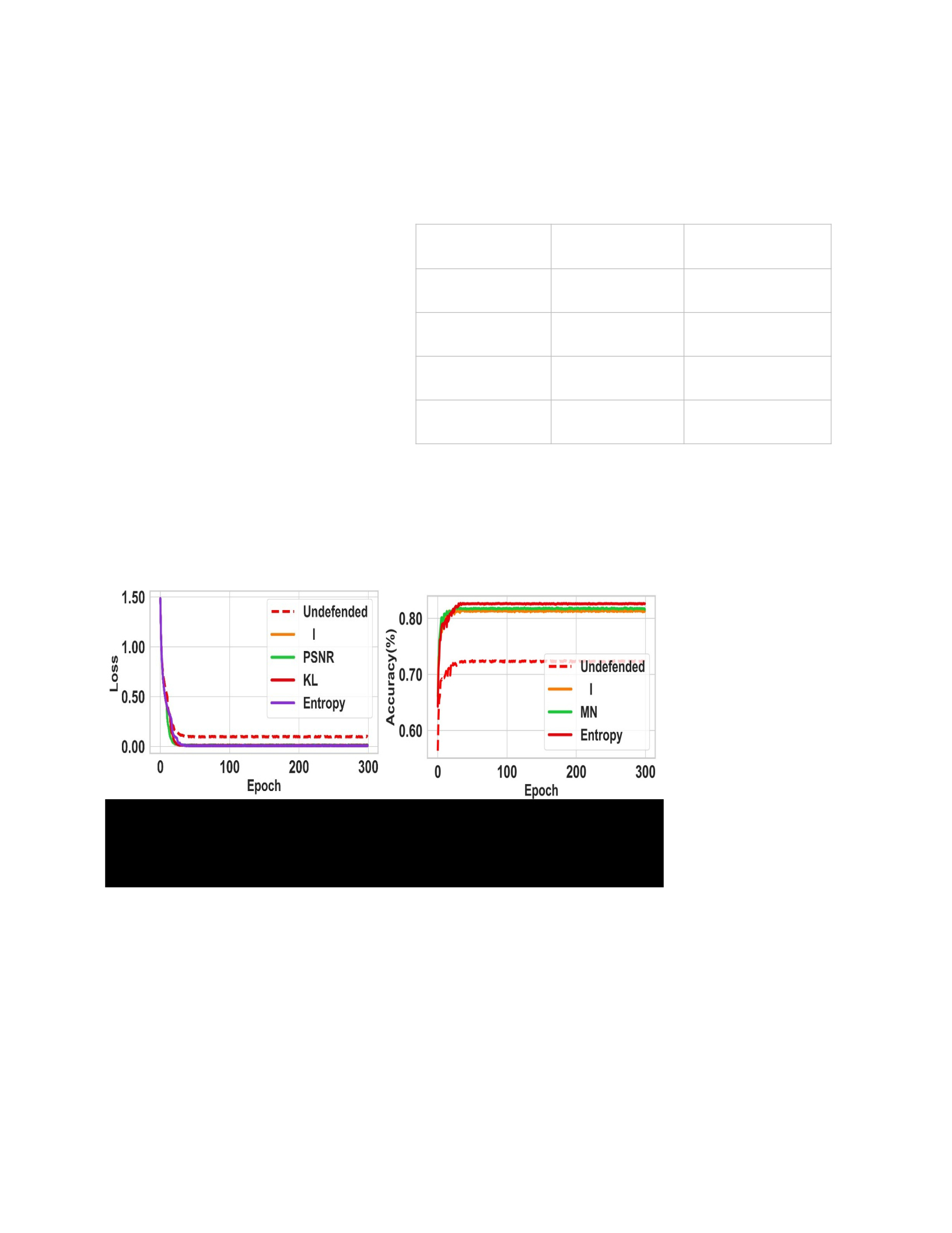
extend the adversary benchmark library, FoolBox’s [186] to implement N-pixel attacks. We
consider N-pixel attacks, where 𝑁 is taken from the interval [1, 16] and patches of size up to
25% of the total image area.
Additional Metrics Table 7.1. Number of Parameters for Different
Models; original (𝑓) and with Modifications (𝑓a+). We
measure the classification accuracy – of
the models on both clean images (𝑎𝑐𝑐
) and adversarial images
𝑎𝑐𝑐$&&$!’. We calculate robustness score
(δ) as the difference between model’s
classification accuracy on clean images and its classification accuracy on adversarial images, δ
= (𝑎𝑐𝑐!"#$% − 𝑎𝑐𝑐$&&$!’). A smaller δ demonstrates greater proactive robustness
against adversarial attacks.
We also measure defense success rate β – the percentage of successfully defended adversarial
attacks. A higher defense success rate indicates a better proactive defense against adversarial
attacks.
Defense Effectiveness
We evaluate the performance of our defense in reducing the effectiveness of N-Pixel and
patch attacks. We use 1, 2, up to 16-pixel coverage for N-pixel. We use adversarial patches –
Figure 7.4. CIFAR10 Training Losses and Success Rates of Defense on EfficientNet. (Left)
Shows the Losses of Defended Model G Using Different Syllabus Configurations and
Undefended Model F. (Right) Shows the Training Success Rates of Both Models Under 1-
Pixel Attack.
Model Original (f) Modified (𝒇𝟑𝑫)
VGG16 143,357,544 183,021,512
ResNet50 25,636,712 74,203,245
InceptionV3 23,851,784 68,104,050
EfficientNetB0 5,330,564 15,900,000
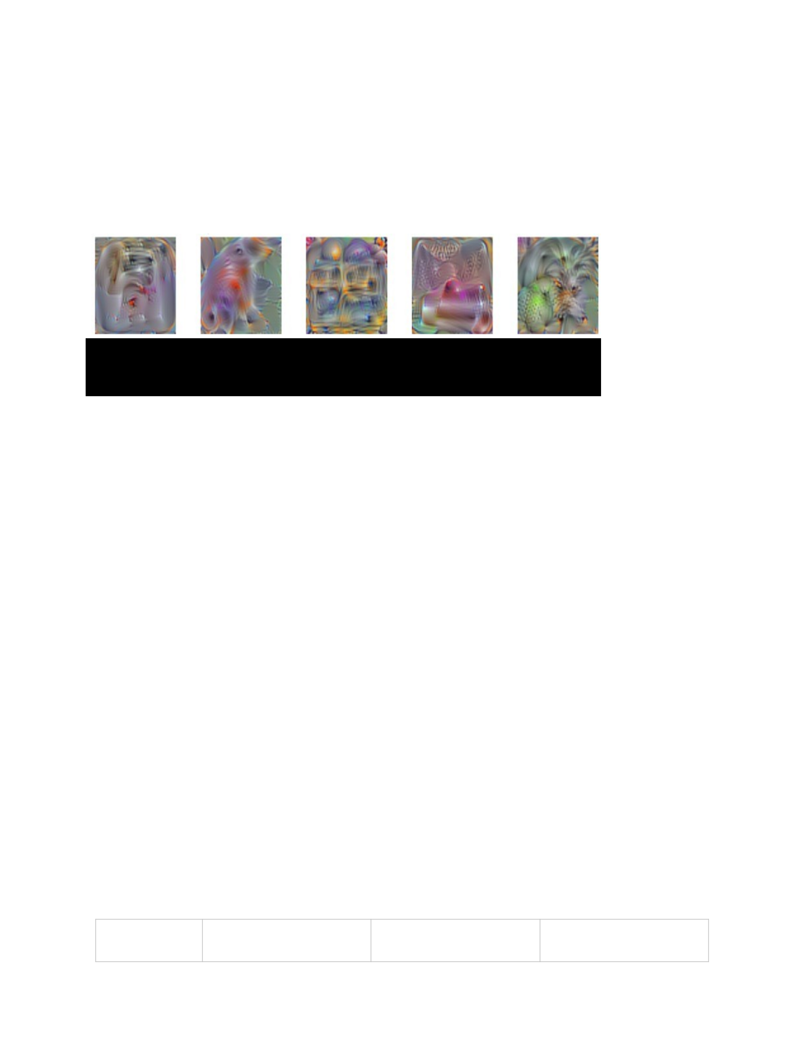
Toaster, School-Bus, Lipstick and Pineapple - synthesized by attack methods A-ADS, covering
up to 25% of the entire image. Our approach is compared with existing defense strategies in
terms of clean accuracy and defense success rate β. We mount such attacks against our defense
(I, KL, H, MN, and PSNR syllabi), and an undefended model as a control. The patch size
(𝑝:, 𝑝H) of the volumization algorithm for all syllabi is set to 16 × 16 pixels. We take
reported results of all baseline defenses for comparison.
CIFAR10, CIFAR100 and ImageNet datasets, with and without our defense mechanisms, for
both clean and attacked test sets. Though the undefended model exhibits good performance
clean data, its performance significantly deteriorates under adversarial attacks. In contrast,
models defended using our approach show resilient performance under adversarial scenarios,
with minimal trade-offs in clean data accuracy.
Notably, the model defended using measure MI outperforms other models under N-Pixel
attack across all datasets. For instance, the model defended using mutual information (I) achieves
attack accuracies of 91.3 (N-Pixel) and 61.6 (APA) on CIFAR10, remarkably higher than the
undefended model’s 43.2 and 44.3, respectively. Similarly, the KL-defended model yields
considerably better attack accuracy on CIFAR100 (73 and 43.2 for N-Pixel and APA
respectively) compared to the undefended version (32.5 and 22.1).
Table 7.2. Generalization Accuracy of EfficientNet on CIFAR10, CIFAR100, And ILSVRC12
Datasets with And Without Our Defense Mechanisms. The Performance is Compared Under
Three Scenarios: Clean Test Sets, Test Sets Under One-Pixel Attack (N-Pixel Where N=1), And
Test Sets Under Patch Attack with a Toaster Sticker (APA).
Defense 𝑨𝒄𝒄𝒄𝒍𝒆𝒂𝒏 𝑨𝒄𝒄𝒂𝒕𝒕𝒂𝒄𝒌(𝑵 −
𝒑𝒊𝒙𝒆𝒍)
𝑨𝒄𝒄𝒂𝒕𝒕𝒂𝒄𝒌(𝑨𝑷𝑨)
Table 7.2 presents a comparison of generalization performance of EfficientNet on
Figure 7.5. Patch Attack Stickers were Used in this Study. Left to Right (Toaster, Goldfish,
Schoolbus, Lipstick and Pineapple) Generated Using the A-ADS Patch Synthesis Method
Highlighted in Brown et al. [2].

CIFAR10 CIFAR100 ISLVRC12 CIFAR10 CIFAR100 ISLVRC12 CIFAR10 CIFAR100 ISLVRC12
Entropy(H) 94 90.5 76.8 85 74 56.8 79 55.2 58.2
MI 96.3 98 79 91.3 70 69 61.6 53 61.2
KL 93 93.2 75 63 73 62.1 65 43.2 36.8
PSNR 89 90.3 76 83.6 51 56 52 53 48.3
Norm(MN) 92 86 75.4 74 51 49.5 42 38 32
Undefended 99 96.8 78.3 43.2 32.5 12.4 44.3 22.1 10.8
Figure 7.6 illustrate the overall robustness (δ) of EfficientNet and Inception against
Npixel and patch attacks, respectively. The plots highlight the dependence of model robustness
on attack size for both defended and undefended models, with the undefended model being 40%
less accurate at worst. Our defense is effective for both architectures at all attack magnitudes.
However, like the undefended model, the performance of our method de- grades as the size of
the attack increases, indicating a shared vulnerability to larger-scale attacks.
As presented in Table 7.3, our proposed defense demonstrates a significant performance
against N-Pixel attack compared to the undefended models. The undefended models exhibit
sharp decline when under attack (𝑨𝒄𝒄𝒂𝒕𝒕𝒂𝒄𝒌 column). Our proposed method (I) not only achieves
high 𝑨𝒄𝒄𝒄𝒍𝒆𝒂𝒏of 96.3% for EfficientNet and 99% for VGG and Inception but also shows a minor
degradation when under attack; by 5%, and 0.4% for Efficient and VGG respectively.
Table 7.3. Accuracy of Models Over the Set of Test Images Without Attacks 𝐀𝐜𝐜𝐜𝐥𝐞𝐚𝐧 And with
Attack 𝐀𝐜𝐜𝐚𝐭𝐭𝐚𝐜𝐤, Reported for All CIFAR10 Classes. Reported As Top 1 Accuracy of 1 Pixel
Attack for the Undefended Model, the Model Defended by our Method (I) And Other Comparable
Approaches. All Images in the Dataset are Attached for this Report.
Defense 𝑨𝒄𝒄𝒄𝒍𝒆𝒂𝒏 𝑨𝒄𝒄𝒂𝒕𝒕𝒂𝒄𝒌
EfficientNet VGG EfficientNet VGG
Undefended 98 98.9 44.3 35.9
I/Ours 96.3 99 91.3 98.6
PSD - 99.53 - 97.8
Liu et al - 89.8 - 91
Comparing mutual information (MI) with the PSD method, our approach has a slightly

lower 𝑨𝒄𝒄𝒄𝒍𝒆𝒂𝒏 for VGG, with a difference of 0.53%, but delivers a better 𝑨𝒄𝒄𝒂𝒕𝒕𝒂𝒄𝒌 for the same
model, with an improvement of 1.2%. When comparing I to Liu et al.’s method, our method
demonstrates a substantial improvement in 𝑨𝒄𝒄𝒄𝒍𝒆𝒂𝒏 for VGG, with a difference of 9.2%, and a
higher 𝑨𝒄𝒄𝒂𝒕𝒕𝒂𝒄𝒌 as well, with an improvement of 4.6%. PSD and Liu et al. do not provide results
for EfficientNet.
Table 7.4 presents defense success rates (β) for various defense methods and ours against
APA on three datasets. For CIFAR10, our methods achieved 95.6% and 96.12% success rates,
while Jujutsu and LGS obtained only 86.5% and 93.2%, respectively. Similarly, for CIFAR100,
our methods reached success rates of 95.43% and 94.3%, outperforming Jujutsu’s 55.7% and
LGS’s 73.7%. In the ImageNet dataset, ours (MI) achieved the highest defense success rate of
89.1%, while PSNR obtained 83.2%, both surpassing Vax-a-Net’s 86.8% and DW’s 65.2% and
Table 7.4. Defense Success Rate (Β) of Various Defense Methods Against APA Covering At
Least 5% of the Image. Adversary Patches: Toaster, Lipstick, Pineapple, And School-Bus Were
Used.
Defense Defense Success Rate(β)
CIFAR10 CIFAR100 ILSVRC12
H/Ours (EfficientNet) 91.3 80.5 -
MI/Ours (ResNet) 95.6 95.43 89.1
PSNR/Ours (Inc) 96.12 94.3 83.2
Jujutsu (ResNet) 86.5 55.7 -
LGS 93.2 73.7 -
V-a-N(VGG) - 91.6 86.8
DW(VGG) - - 65.2
DW(Inc) - - 66.2
ECViT-B 47.39 - 41.7
66.2% for VGG and Inception models, respectively. Not all methods have reported results for
every dataset, limiting a comprehensive comparison of their effectiveness.
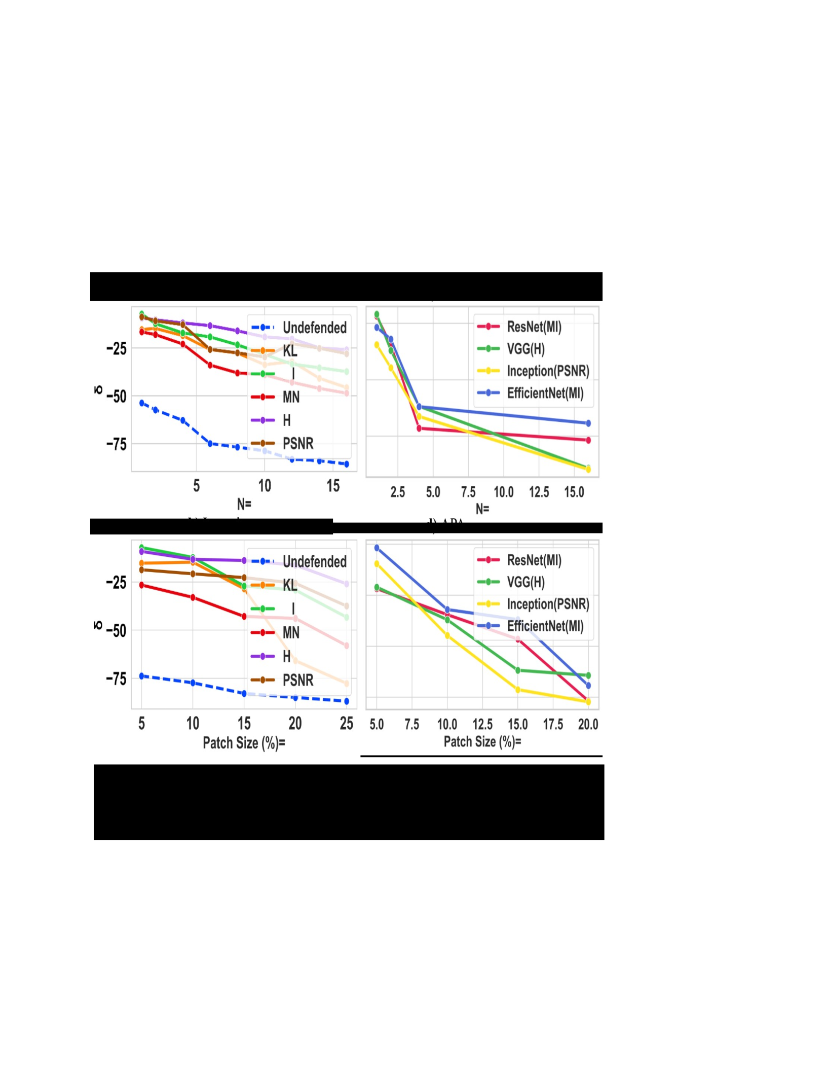
Attack Size Impact on Model Performance
Figure 7.6 show the defense success rate (β) for all four models under N-pixel and APA
attacks, respectively, using a depth of 16 for the volumizer algorithm in the decreases when
attacked pixels surpass the patch size of the volume. This is due to the volumization algorithm’s
design, which focuses on small attacks and becomes less effective when perturbations exceed the
patch size or span multiple slices. This limitation is more prominent if the attack covers a large
image portion, potentially obscuring important object details.
Class Generalization
Figure 7.7 depicts VGG generalization performance on CIFAR10 test data. The
undefended model exhibits an AUC of 0.5, while the defended model achieves an AUC of 0.69
under 1-pixel attack while the same model achieves AUC of 0.65 under APA. This indicates that
Figure 7.6. (a) EfficientNet Robustness as a Function of N - Number of Pixels Attacked, (b)
Inception Robustness Against APA As a Function of Patch Size, (c) Defense Success Rate of
Various Models as a Function of N-Pixel Attack Magnitude, (d) Defense Success Rate Β of Various
Models as a Function of APA Attack Magnitude.

the defended model shows improved performance in terms of class generalization compared to
the undefended model. These plots suggest that the defended model has better discriminative
power and can effectively distinguish between different classes in the CIFAR10 dataset when
under 1 pixel and APA attacks. This improvement in AUC demonstrates the effectiveness of our
proposed approach in enhancing the model’s class generalization capabilities when under
localized universal attacks.
Ablation Study
We conduct an ablation study to assess the impact of volume depth and curriculum
learning in our defense methodology.
Impact of CL on Defense Success Rate
For this experiment, we train our models with and without the curriculum learning phase
and compare the results with the fully trained models. The results are presented in Table 7.5.
The first scenario we tested was our method without CL but with the volumizer (I-Vol).
The performance under this configuration was reasonably good, with the 𝐴𝑐𝑐!"#$% being 93.7%,
97.2%, and 97.4% for EfficientNet, VGG, and Inception, respectively. However, the
𝐴𝑐𝑐$&&$!’was markedly lower, specifically 81.6% for EfficientNet, 89.7% for VGG, and 85.2%
for Inception. Compared to the full method (I), the 𝐴𝑐𝑐$&&$!’ was lower by 9.7%, 8.9%, and
10.9%, respectively. This indicates the effectiveness of Curriculum Learning in improving the
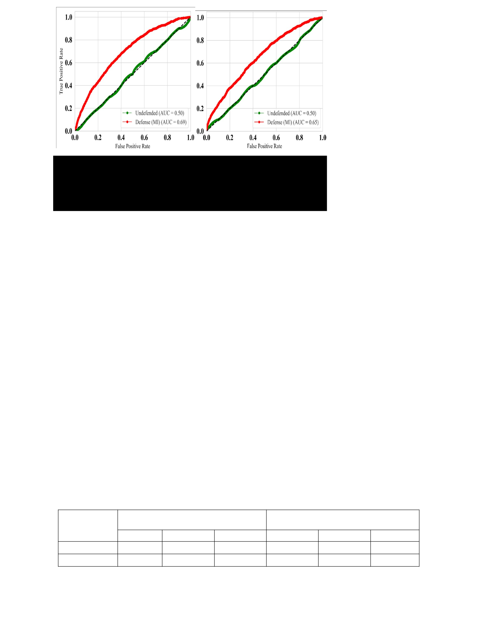
model’s robustness against adversarial attacks. Second, we studied the effect of Curriculum
Learning without the volumizer (I-CL). This configuration achieved even higher 𝐴𝑐𝑐!"#$%
scores, specifically 97.9%, 99.4%, and 98.6% for EfficientNet, VGG, and Inception, respectively.
However, the 𝐴𝑐𝑐$&&$!’ suffered significantly without the volumizer. For EfficientNet, VGG,
and Inception, the 𝐴𝑐𝑐$&&$!’ were 56.8%, 38.1%, and 12.3%, respectively, revealing drops of
34.5%, 60.5%, and 83.8% compared to the full I syllabus. This demonstrates the vital role the
volumizer plays in enhancing the model’s resilience to adversarial attacks.
Lastly, our fully implemented method (I), incorporating both Curriculum Learning and the
volumizer, consistently outperformed the other configurations in terms of 𝐴𝑐𝑐$&&$!’, achieving
91.3%, 98.6%, and 96.12% for EfficientNet, VGG, and Inception, respectively. These figures
indicate the combined effect of both components in improving the model’s resilience to
adversarial attacks.
Table 7.5. Impact of Curriculum Learning and Volumizer: 𝐀𝐜𝐜𝐜𝐥𝐞𝐚𝐧 And 𝐀𝐜𝐜𝐚𝐭𝐭𝐚𝐜𝐤 For
Models Trained Without Curriculum Learning (I-Vol), Models Trained with Curriculum Learning
but Without Volumizer (I-CL), And Fully Trained Models (I).
Method 𝑨𝒄𝒄𝒄𝒍𝒆
𝒂𝒏 𝑨𝒄𝒄𝒂𝒕𝒕𝒂
𝒄𝒌
EffNet VGG Inception EffNet VGG Inception
I-Vol 93.7 97.2 97.4 90.6 95.7 95.2
I-CL 97.9 99.4 98.6 56.8 38.1 12.3
Figure 7.7. (Left) ROC of VGG Model Under 1-Pixel Attack. (Right) ROC of VGG Model
Under APA of Size 8 by 8 Pixels. Class Generalization Performance Comparison Between
Defended and Undefended VGG on CIFAR10 Test Set. the Plots are Micro Average ROC Curve
Across the 10 Classes.
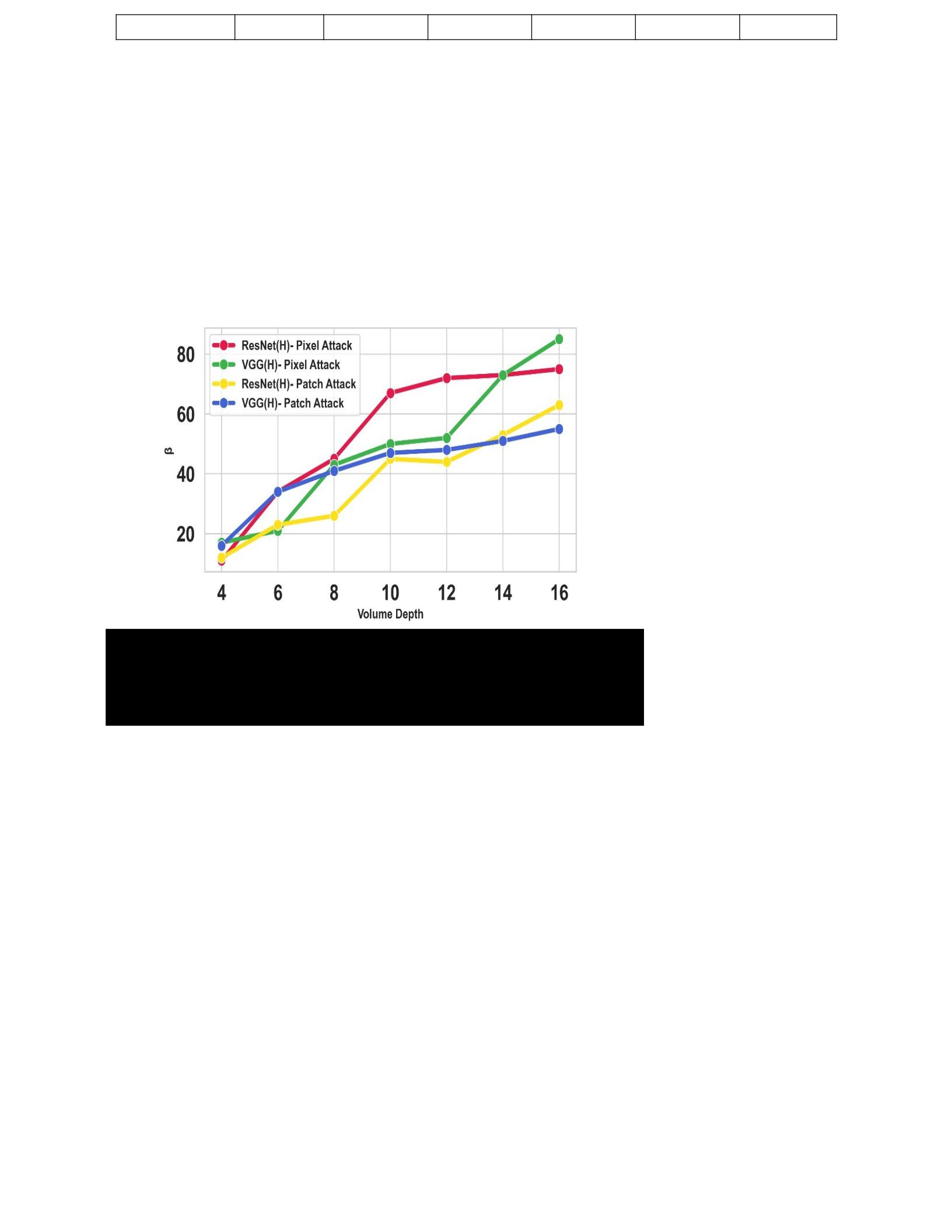
I 96.3 99 99 91.3 98.6 96.12
Impact of Patch Size on Defense Success Rate
We investigated the relationship between patch size and defense success rate by analyzing
how changes in slice size affect the effectiveness of the defense mechanism.
Figure 7.8 depicts this relationship, showing that as the volume depth increases, the
defense success rate also increases. This can be attributed to a few factors. Smaller slices allow
the model to focus on more localized portions of the image, enabling a finer resolution of local
sensitivity to small perturbations, a characteristic of localized adversarial attacks.
Additionally, a larger depth allows for more granular learning and effectively increases
the diversity of the training data, leading to a model that generalizes better in non-adversarial
setting and exhibits higher resistance to localized attacks.
Timing Information
Inference and training time comparisons between our method and undefended models are
presented in Table 7.6. An inference overhead for a model protected with our method is
noticeable compared to the undefended models– around 6 milliseconds on average across all
features that can aid in detecting subtle adversarial perturbations. It also heightens the
model’s
Figure 7.8. Impact of Patch Size (Volume Depth) on Defense Success Rate (Β) Against Pixel
Attack on CIFAR10 Dataset. the Training Samples Are of Shape (32, 32, 3). We Generated
Volumes Staring with a Patch of Size 16 by 16 With Depth 4, All the Way to a Patch Size of 4
by 4 With Depth 16.

three models. This increased latency is primarily due to the modifications made to the model
architecture to accommodate our defense strategy. Additionally, our defense incurs a significant
overhead during training. Depending on the size of the dataset, the additional training time can
span from hours to days. However, this process only needs to be run once, as does preprocessing
dataset a priori. All inference runs used an NVIDIA RTX A4000, while training was conducted
on a node equipped with four RTX A100 GPUs. Despite the increased computational demands,
the benefits of enhanced security provided by our defense method offer a worthwhile trade-off.
Qualitative Results
Figure 7.9 presents results of attacked CIFAR10 dataset. The implemented defense
strategies are Mutual Information (I) and Entropy (H) syllabus. The models were subjected to 1,
2, 4-, 3-, 5- or 8-pixel attacks. All patch stickers in the figures are 8 by 8 pixels covering about
5% of the total image. Each image is labeled with Undefended, and the defense mechanism used
along with volume depth.
Table 7.6. Inference Time (ms) For VGG, Resnet, And
Inception Trained on ImageNet and the Same Model with Our Defense Based
on I Syllabus And a 16 Depth Volumized Inputs.
Method VGG ResNet Inception
Undefended 0.12 0.14 0.09
I/Ours 0.23 0.18 0.16
Volume Visualization
This section presents the visualizations of volumes generated using different metrics. The
image (Figure 3), taken from the ImageNet dataset is scaled up to 1024 by 1024 for visualization
purposes. Figures 4 and 5 show volumes generated using Entropy with slice sizes of 128 by 128
and 256 × 256 respectively. Only the first and last 8 slices with their rank and metric
values are plotted. Figure 7.12 showcases the volume generated using the mutual information
(MI) metric. The slice size used in this case is 64 × 64, resulting in a volume shape of (64,64, 3,
256). The reference image is highlighted with dotted blue lines.

These provide insights into the structure and characteristics of the generated volumes,
highlighting the effectiveness of the different metrics and patch sizes in capturing relevant
information. As can be seen in the figures, slices that have highly salient objects are prioritized,
ensuring that the generated volumes focus on preserving important features and capturing
significant visual patterns early in the feature extraction phase. By emphasizing slices with
Figure 7.10. Original Image (x), shape = (1024, 1024, 3).
highly salient objects, the volumizer helps identify and understand the critical regions that are
vulnerable to attacks. This approach also aids the curriculum learning process by presenting
visually rich and informative instances early on. The combination of prioritizing salient objects
and adopting curriculum learning strategies provides an approach to enhance the network’s
robustness, and adaptability in complex visual tasks.
Summary and Conclusion
We presented a robust training approach to proactively defend against localized
adversarial attacks without degrading the performance of the model on clean data. In the process
of achieving this, we developed a volumization algorithm that converts 2D images into a 3D
volumetric representation by extracting and ranking patches based on specific metrics. This
volumization technique preserves spatial relationships within the image, making it more resilient
Figure 7.11. 𝑥( generated using MI,shape=(64,64, 3, 256). The reference image is
highlighted.
Figure 7.12.𝑥(GeneratedUsingEntropy,Shape=(256,256,3,16).

to adversarial perturbations. We also use a deep curriculum learning optimization strategy that
orders the training samples in a batch based on their complexity or difficulty, allowing the model
to learn progressively from simpler to more complex samples. This approach enhances the
model's ability to generalize in any setting. By integrating the two into popular and contemporary
CNN architectures, we demonstrated the efficacy of our proposed method in defending against
N-pixel and patch attacks. The experimental results showed improved robustness against
perturbations while maintaining high performance on clean data, validating the effectiveness of
our approach in enhancing the resilience of image classification models against localized
adversarial attacks.
CHAPTER 8
CONCLUSION, LIMITATIONS, AND FUTURE WORK
This thesis introduced a curriculum-based framework to enhance model training
efficiency through three main innovations: curriculum learning for optimized sample sequencing,
patchbased preprocessing with PROSIS-2D for enhanced feature extraction, and volumization
with PROSIS-3D for increased resilience against adversarial attacks. Together, these methods

create a comprehensive approach that significantly reduces computational demands while
maintaining robust performance across varied datasets and tasks.
The curriculum learning method prioritizes training samples using a concrete metric such
as Entropy, enabling the model to learn essential patterns faster. By structuring the learning
sequence, the curriculum approach demonstrated faster convergence and improved sample
utilization, proving especially effective on benchmark datasets like CIFAR-10 and CIFAR-100.
This targeted learning path highlights the efficiency gains achievable when training is structured
to emphasize sample progression based on some inherent characteristics.
The introduction of PROSIS-2D leverages patch-based preprocessing to reorder spatial
features within each image, allowing for more efficient feature extraction without altering model
architecture. By focusing on local spatial relations, PROSIS-2D minimizes redundant
computations and accelerates convergence, making it a valuable tool for applications where
training time and computational resources are constrained.
Finally, PROSIS-3D applies volumization to enhance model security, particularly against
adversarial attacks. By representing images as 3D volumes, this method strengthens spatial
coherence within the model’s feature extraction layers, thus mitigating the impact of localized
perturbations. The experimental results demonstrate that volumized data representation
significantly boosts the model's robustness, underscoring PROSIS-3D's potential for secure deep
learning applications.
Collectively, these techniques form an integrated framework that optimizes training
efficiency and enhances security, making it highly applicable to domains requiring
highperformance, resource-efficient models.
Limitations
Despite its demonstrated effectiveness, the curriculum-based framework developed in this
thesis has several limitations that present opportunities for improvement. First, a central aspect of
the framework is its dependency on sample ranking metrics, which serve as the foundation for

constructing an efficient training syllabus. These metrics are designed to capture the inherent
characteristics of each sample, such as its representativeness, uniqueness, or importance within
the dataset. However, there is a risk that these metrics may not fully capture the complexity or
informativeness of each sample, particularly in datasets with high variability or intricate
underlying patterns. If the metrics fail to accurately assess which samples are most valuable for
training, the model may end up prioritizing less impactful samples or skipping those that could
contribute more significantly to learning. This misalignment could reduce the framework’s
intended efficiency benefits, as the model may require additional iterations or encounter slower
convergence.
Moreover, the process of generating and evaluating custom syllabi for each dataset can
introduce a considerable computational load, particularly for large-scale datasets. Creating a
syllabus requires ranking each sample and organizing them into a structured training sequence, a
task that is computationally intensive and becomes increasingly so with larger datasets. After
syllabus creation, the framework includes an evaluation phase to determine the syllabus’s
effectiveness, potentially requiring additional iterations to refine the syllabus if the initial
structure does not yield optimal efficiency gains. For very large datasets, the combination of
these steps— ranking, syllabus structuring, and evaluation—could significantly offset the
intended computational efficiency, especially if the syllabus needs frequent recalibration. This
additional overhead could limit the practicality of the framework for time-sensitive or resource-
constrained applications, suggesting the need for lightweight or automated syllabus generation
techniques to improve scalability.
Another notable limitation is the current framework’s preliminary handling of 3D data
through PROSIS-3D, which has been effective in introducing volumization but still faces
challenges in complex, high-dimensional data environments like medical imaging (e.g., MRI or
CT scans). PROSIS-3D was developed to extend the curriculum-based approach to 3D data by
representing images as volumetric structures, enhancing spatial coherence and improving

resilience against adversarial attacks. While this volumization strategy shows promise, it
currently addresses only a subset of the challenges associated with 3D data processing.
3D data presents additional complexities compared to 2D data due to its inherent spatial
and structural depth, as each sample comprises multiple layers (slices) that contain
interdependent information across three dimensions. Effectively capturing the complexity and
relevance of each volumetric sample requires advanced ranking metrics that account not only for
individual slices but also for the relationships across slices. In PROSIS-3D’s current
implementation, metrics primarily focus on individual layer characteristics, which may not fully
capture the volumetric dependencies that are crucial for accurate representation and efficient
learning in medical imaging tasks. This limitation indicates that future iterations of the
framework will require metrics that can better represent the layered coherence and spatial
relationships within 3D data.
Additionally, the syllabus generation methods in PROSIS-3D must evolve to
accommodate the structural dependencies and coherence that exist between slices in 3D volumes.
Designing a syllabus that optimizes the learning sequence for such volumetric data demands
more sophisticated algorithms that preserve both global and local spatial information. Without
these enhancements, the framework may struggle to achieve the same level of training efficiency
for 3D data as it does for 2D data, potentially limiting its effectiveness in domains like medical
imaging, where volumetric data is standard and computational efficiency is essential.
These 3D-specific requirements—robust ranking metrics for volumetric dependencies and
advanced syllabus generation methods that account for spatial coherence across slices—are
critical areas for future development. Without such adaptations, PROSIS-3D may continue to
face limitations in scaling its efficiency gains and accuracy for 3D data applications, particularly
in resource-intensive fields like medical imaging.

Future Work
Future research can build on this framework in several promising directions, alongside
addressing its current limitations. A key short-term objective is to extend the curriculum
framework to 3D volumetric data for medical imaging applications such as MRI analysis. By
adapting the framework to handle the inherent complexity of 3D data, this expansion would
improve training efficiency for high-dimensional, resource-intensive tasks, enabling more
effective learning from volumetric structures and spatial dependencies within medical images.
Another critical focus is on automated syllabus generation for various dataset-model
combinations, which would result in a comprehensive library of optimized syllabi tailored to the
specific characteristics of each dataset and model pairing. This resource would streamline the
training process across a diverse range of tasks and model architectures, enhancing both
efficiency and adaptability by eliminating the need for manual syllabus design.
Finally, in the long term, future work will explore adaptive learning paths using
reinforcement learning, allowing for real-time syllabus adjustments based on ongoing model
performance. Such a dynamic approach could significantly boost training efficiency by
continually refining the curriculum as training progresses, making the framework more
responsive to evolving data and model requirements. Together, these advancements would enable
a more flexible, robust, and efficient training framework that can adapt to a wide array of data
types and model architectures.


