


3.
MODELLING GALAXIES
37
v
·
Luminosity-velocity relations:
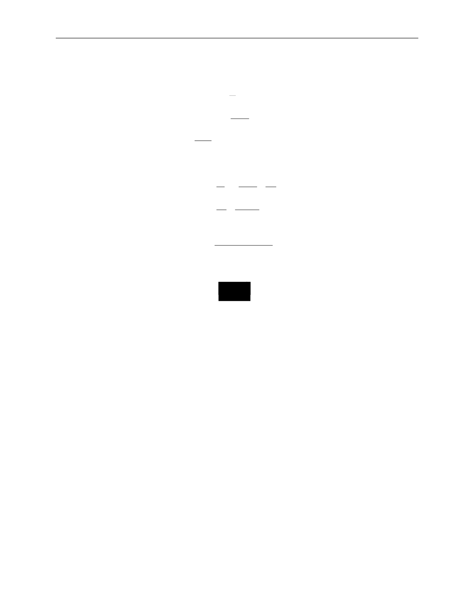
We can relate properties of a galaxy to observables through several equations:
R
θ
=
(apparent size)
d
L
F
=
4πd
2
(158)
v
2
=
GM .
R
Introducing surface brightness Σ
F
L
d
2
Σ =
=
θ
2
4πd
2
R
2
(159)
L
v
4
then
=
4π
·
G2M 2
v
4
L =
Σ4πG
2
(M/L)
2
.
(160)
If we assume, for a given class of galaxies, that the surface brightness and the mass-to-light
ratio are the same, then
.
(161)
This introduces two important relations.
The Tully-Fischer relation is used for spiral galaxies and relates the maximum velocity in
the rotation curve
v
max
, which can be measured from HII spectra, and the luminosity:
4
max
.
(162)
The Faber-Jackson relation is used for ellipticals and relates the velocity dispersion
σ
v
to the
luminosity:
L
∝
σ
4
.
(163)
Thus, we can get an estimate of the intrinsic luminosity of a galaxy be measuring stel-
lar velocities. The constant of proportionality is roughly
L
∗
/(220 km/s)
4
, where
L
∗
is the
characteristic galaxy luminosity.
3.C
Phase-space distribution function
We have described the individual orbits in a potential, but this is not sufficient to describe
galactic dynamics. We want information of the configuration of all particles. Each star is
described by its position
→
x
and velocity
→
v
,
and we need to know this for all stars, i.e. how
stars are distributed in the 6D phase space
(
→
x
,
→
v
)
.
We define a phase-space distribution function
f
(
→
x
,
→
v
,
t)d3
→
x
d
3
→
v
(164)
∝
L
∝
v
3.
MODELLING GALAXIES
38
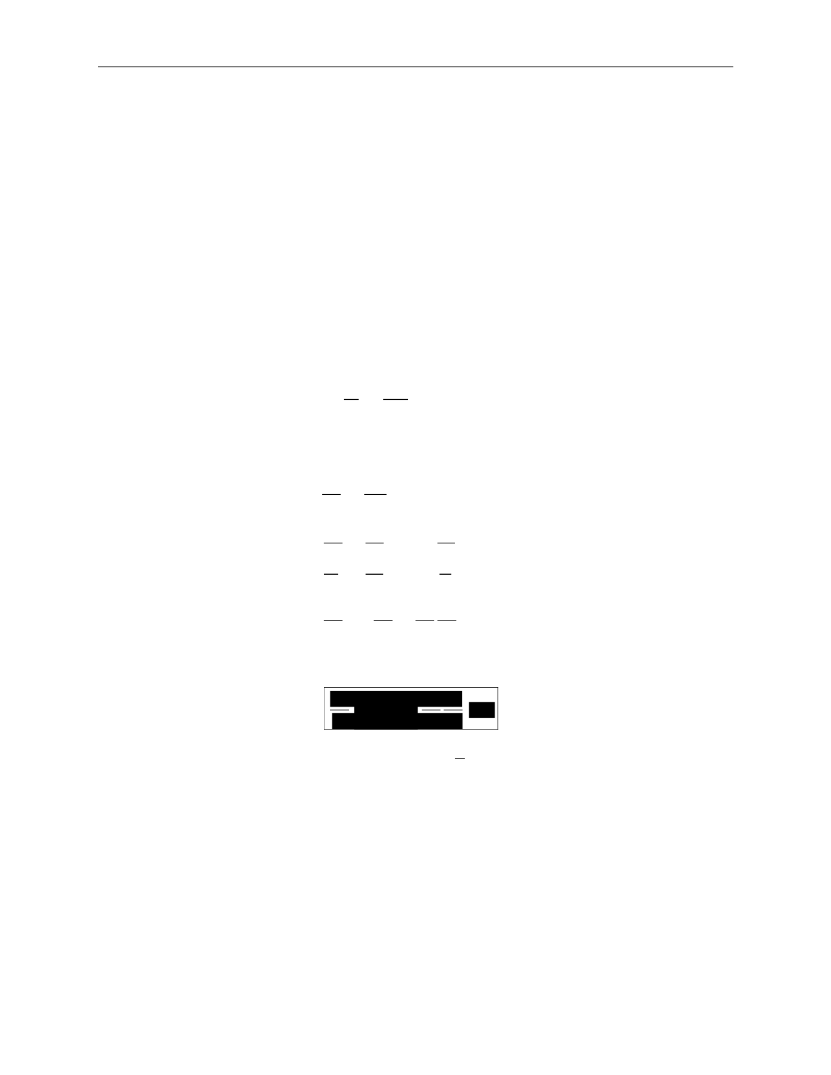
∈
dt
as the probability that at time
t
, a randomly chosen star has
(
→
x
∗
,
→
v
∗
)
([
→
x
,
→
x
+
d
→
x
]
,
[
→
v
,
→
v
+
d
→
v])
.
This
means
that
the function must be normalized for all
t
, i.e.
∫
f
(
→
x
,
→
v
,
t)d
3
→
x
d
3
→
v
= 1 .
(165)
Collisionless
Boltzmann
equation
:
We want to describe the time evolution of
f
(
→
x
,
→
v
,
t)
. Since probability cannot be destroyed,
the 6D continuity equation must hold.
We define the 6D phase-space vector
then
w
→
=
(
→
x
,
→
v
)
(166)
∂f
+
∂
f
w
→
˙
=
0 .
(167)
∂t
∂w
→
This is the same form as the standard 3D continuity equation. We can rewrite this by
expanding out
w
→
and using velocity
→
v
=
→
x
˙
and acceleration
→
a
=
→
v
˙
:
0
= ∂f +
∂
f
w
→
˙
∂t
∂w
→
∂f
∂
=
+
∂t
∂
→
x
(
f
→
x
˙
) +
∂
(
f
→
v
˙
)
∂
→
v
(168)
∂f
∂
∂
=
+
(
f
→
v
)
+
f
(
−
∇
→
φ)
∂t
∂
→
x
∂
→
v
∂f
∂f
∂φ
∂f
=
∂t
+
→
v
∂
→
x
−
∂
→
x
∂
→
v
.
This gives us the collisionless Boltzmann equation (CBE):
.
(169)
Note that another way to see this is by writing out
df
= 0
and taking the limits
lim
→x
→∞
= 0
and
lim
→v
→∞
= 0
.
General Jeans equations:
A solution to the collisionless Boltzmann equation is difficult to obtain, so we instead study
moments of the CBE and the phase-space distribution.
Moments of the phase-space density give us some average quantities of the system.
a)
The first moment gives the density
n
of the system:
n
=
∫
f
d
3
→
v
.
(170)
∂t
−

3.
MODELLING GALAXIES
39
ij
∫
—
∫
∫
∫
±∞
—
i
n
i
i
j
n
i
j
∂
→
x
∂
→
v
∂
→
x
∂
→
v
∂
→
x
→v=
−∞
j
∂t
j
∂
→
x
j
∂
→
x
∂
→
v
2
b)
The second moment gives the average velocity
v
¯
i
:
v
¯
=
1
∫
v
f
d
3
→
v
.
(171)
c)
The third moment gives the velocity dispersion
σ
2
:
v v
=
1
∫
v v
f
d
3
→
v
ij
=
v
i
v
j
−
v
¯
i
v
¯
j
=
(v
i
−
v
¯
i
)(
v
j
−
v
¯
j
)
.
We now examine moments of the collisionless Boltzmann equation more closely. We break
each integral into three terms to simplify each individually.
a)
First moment:
d
3
→
v
∂f
∂t
∂f
+
→
v
∂
→
x
∂φ
∂f
=
0
∂
→
x
∂
→
v
∫
d
3
→
v
∂f +
∫
d
3
→
v
→
v
∂f
−
∫
d
3
→
v
∂φ
∂f =
0 (173)
∂t
` ˛
1
¸ x
∂
→
x
` ˛
2
¸ x
∂
→
x
∂
→
v
` ˛
3
¸ x
:
d
3
→
v
∂f =
∂
∂t ∂t
d
3
→
v
f
=
∂n
∂t
:
d
3
→
v
→
v
∂f
∂
→
x
∂
=
∂
→
x
d3
→
v
→
v
f
=
∂
∂
→
x
n
→
v
¯
=
Σ
∂
∂x
i
(
n
v
¯
i
)
(174)
:
∫
d
3
→
v
∂φ
∂f
=
∂φ
∫
d
3
→
v
∂f
=
∂φ [f ]
→v=+
∞
=
0
For the third term, we used the fact that phase-space distribution goes to 0 at
for
physical systems.
This gives us the 3D continuity equation:
b)
Second moment:
.
(175)
∫
d
3
→
v
vj
∂f
∂f
+
→
v
∂t
∂
→
x
∂φ
∂f
=
0
∂
→
x
∂
→
v
∫
d
3
→
v
v
∂f +
∫
d
3
→
v
v
→
v
∂f
−
∫
d
3
→
v
v
∂φ
∂f
=
0
(176)
` ˛
1
¸ x ` ˛
2
¸ x ` ˛
3
¸ x
1
2
3
∂n ∂
∂t
0
σ
∫
i
(172)

3.
MODELLING GALAXIES
40
ij
Σ
∫
i
∂x
∂x
j
∂t
∂t
j
∂t
j
∂t
∂t
∂x
i
∂t
∂t
j
∂x
i
using the continuity equation ∂n
=
−
Σ
∂
(
n
v
¯
)
j
∂
→
x
i
∂x
i
∂x
i
j
i
i
∂x
ij
i
j
∂x
j
∂v
j
v
i
=
−∞
i
∂v
∂t
∂x
i
∂x
ij
i
j
∂x
i
`
i
i
ij
i
∂x
i
∂v
:
∫
d
3
→
v
v
∂f =
∂
∫
d
3
→
v
v
f =
∂
(
n
v
¯
) =
∂
n
v
¯
+
n
∂
v
¯
j
=
−
v
¯
Σ
∂
(
n
v
¯
) +
n
∂
v
¯
j
=
n
∂
v
¯
j
−
v
¯
Σ
∂
(
n
v
¯
)
∂t
∂x
i
i
to go from the first line to the second
:
∫
d
3
→
v
v
→
v
∂f
=
∫
d
3
→
v
v
Σ
v
∂f =
Σ
∂
∫
d
3
→
v
v v
f
= nv
j
v
i
`
= n
˛ ¸
σ
2
+
x
v
¯
i
v
¯
j
=
Σ
∂
n
σ
2
+
v
¯
v
¯
:
∫
d
3
→
v
v
∂φ
∂f
=
∫
d
3
→
v
v
Σ
∂φ
∂f
=
Σ
∂φ
∫
d
3
→
v
v
∂f
(177)
((k, l, i) are permutations of (1, 2, 3))
=
∂φ
dv
∂x
k
∫
dv
l
∫
dv
i
∂f
v
j
∂v
=
[v
f
]
˛
v
¸
i
=+
∞
−
x
∫
dv ∂v
j
f
= 0
−
∫
dv
i
δ
ij
f
=
−
Σ
∂φ
∫
dv
∫
dv
l
∫
dv
i
δ
ij
f
i
i
=
−
Σ
∂φ
∫
d
3
→
v
δ
f
i
i
∂φ
=
−
n∂x
j
Plugging each term back in, we get
n
∂
v
¯
j
−
v
¯
Σ
∂
(
n
v
¯
) +
Σ
∂
n
σ
2
+
v
¯
v
¯
+
n
∂φ
=
0
(178)
i
i
i
i
i
i
i
i
i
i
i
1
2
3
j
j
i
j
i
i
j
∂
→
x
∂
→
v
j
i
i
i
j
k

3.
MODELLING GALAXIES
41
Σ
v
¯
2
2
∂t
j
∂x
i
∂x
ij
i
∂x
i
i
j
∂x
j
=
(
n
v
¯
i
)
∂
x
v
¯
j
+
v
¯
j
∂x
(
n
v
¯
i
)
∂t
i
∂x
j
∂x
ij
∂x
—
1
Σ
∂(nσ
ij
) :
pressure
∂t
i
i
i
i
i
i
i
i
j
which we can rewrite
n
∂
v
¯
j
−
v
¯
Σ
∂
(
n
v
¯
)
+
Σ
∂
(nσ
2
)+
Σ
∂
(
n
v
¯
v
¯
)
+n
∂φ
=
0
`
Σ˛¸
∂
x
Σ
∂
(179)
where the two underlined terms cancel. This gives us
n
∂
v
¯
j
+
Σ
(
n
v
¯
)
∂
v
¯
+
Σ
∂
(nσ
2
) +
n
∂φ
=
0 .
(180)
This is the Jeans equation, often written
(181)
Each term can be physically interpreted:
∂
v
¯
j
∂t
∂
v
¯
j
i
∂x
: acceleration of fluid
: kinematic viscosity/shear
i
i
2
(182)
n
∂x
i
∂φ
−
∂x
j
: gravity
Jeans
equations
in
spherical
systems
:
We can convert to spherical coordinates and take velocity moments to give us the Jeans
equations in spherical coordinates. This is complicated!
To simplify, we take the radial Jeans equation and focus on steady-state symmetric systems.
Implications:
∂
=
0
since we have steady state
•
v
¯
r
=
0
otherwise we have net radial motion
•
v
¯
θ
=
v
¯
φ
=
0
or the symmetry is broken
•
σ
rφ
=
0
or the symmetry is broken
2
•
σ
φφ
≡
σ
or the symmetry is broken.
2
2
rθ
θθ
t
∂φ
1
∂t
•
=
σ
=
σ
i
i
i
i
i
3.
MODELLING GALAXIES
42
2
2
2
2
t
t
t
— t
2
rr
rσ
rσ
rσ
rr
r
∂r
G
n
∂r
rr
—
dr
2
—
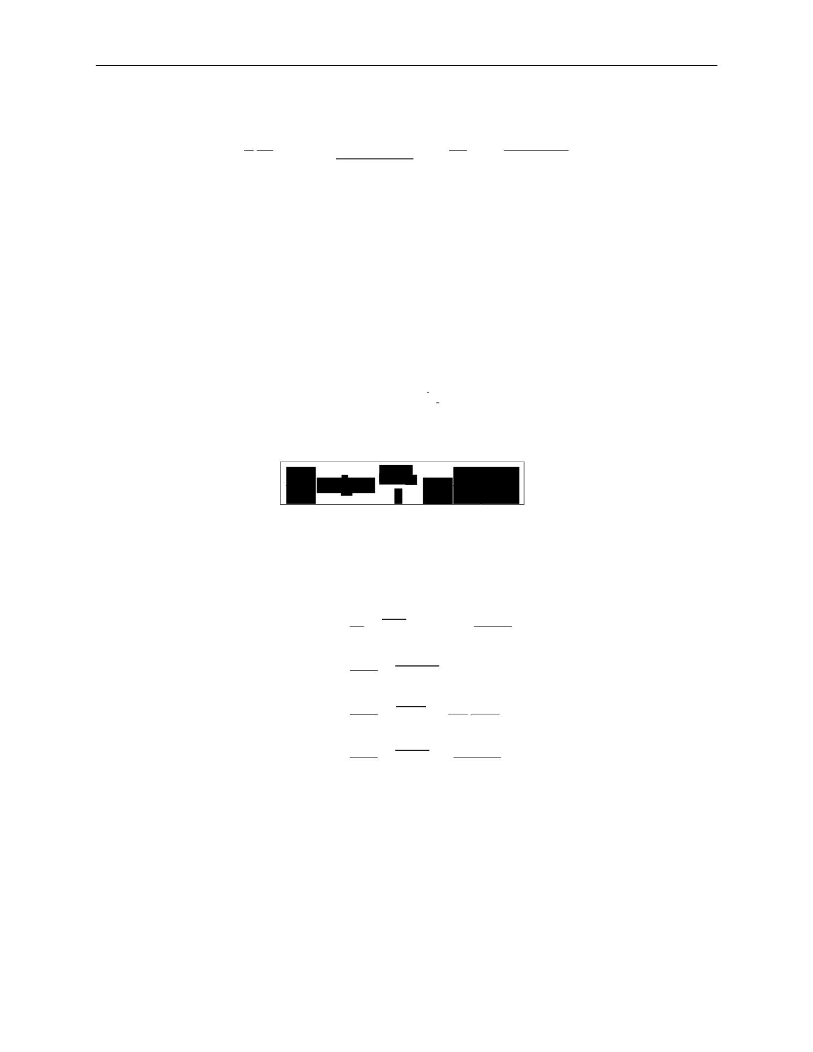
The simplified Jeans equation is:
1 ∂ 2(σ2
− σ ) ∂φ
GM (< r)
(nσ
2
) +
rr
t
=
−
=
−
(183)
where we’ve plugged in gravity as the force.
We have three limits we can look at:
•
σ
rr
•
σ
rr
•
σ
rr
σ
2
: nearly circular orbits
σ
2
: nearly radial orbits
= σ
2
: isotropic orbits
We define the anisotropy parameter:
σ
2
β
=
1
rr
(184)
which gives us a useful form of the Jeans equation for observations:
.
(185)
This depends only on radial components with uncertainty from
β
, assuming spherical sym-
metry and a steady-state system.
This can be simplified further to get mass estimates:
r2
1 ∂ 2 2βσ2
M (< r)
=
−
(nσ
)
+
2
=
−
rr
r
∂
(nσ
2
)
+
2β
G
2
=
rr
G
2
rr
r dn
+
n dr
rr
r
dσ
2
rr
+
2β
rr
(186)
2
=
rr
G
d ln n
+
d ln r
d ln σ2
rr
+
2β
d ln r
where the last line can be measured with observations.
Stability of stellar systems
The existence of equilibrium solutions to the collisionless Boltzmann equation does not assure stability.
Real stellar systems are subject to perturbations. What is important for stability?
1 ∂
2βσ2
σ
nσ
σ
n
∂r
r
2
r
∂r
3.
MODELLING GALAXIES
38
v
·
Luminosity-velocity relations:
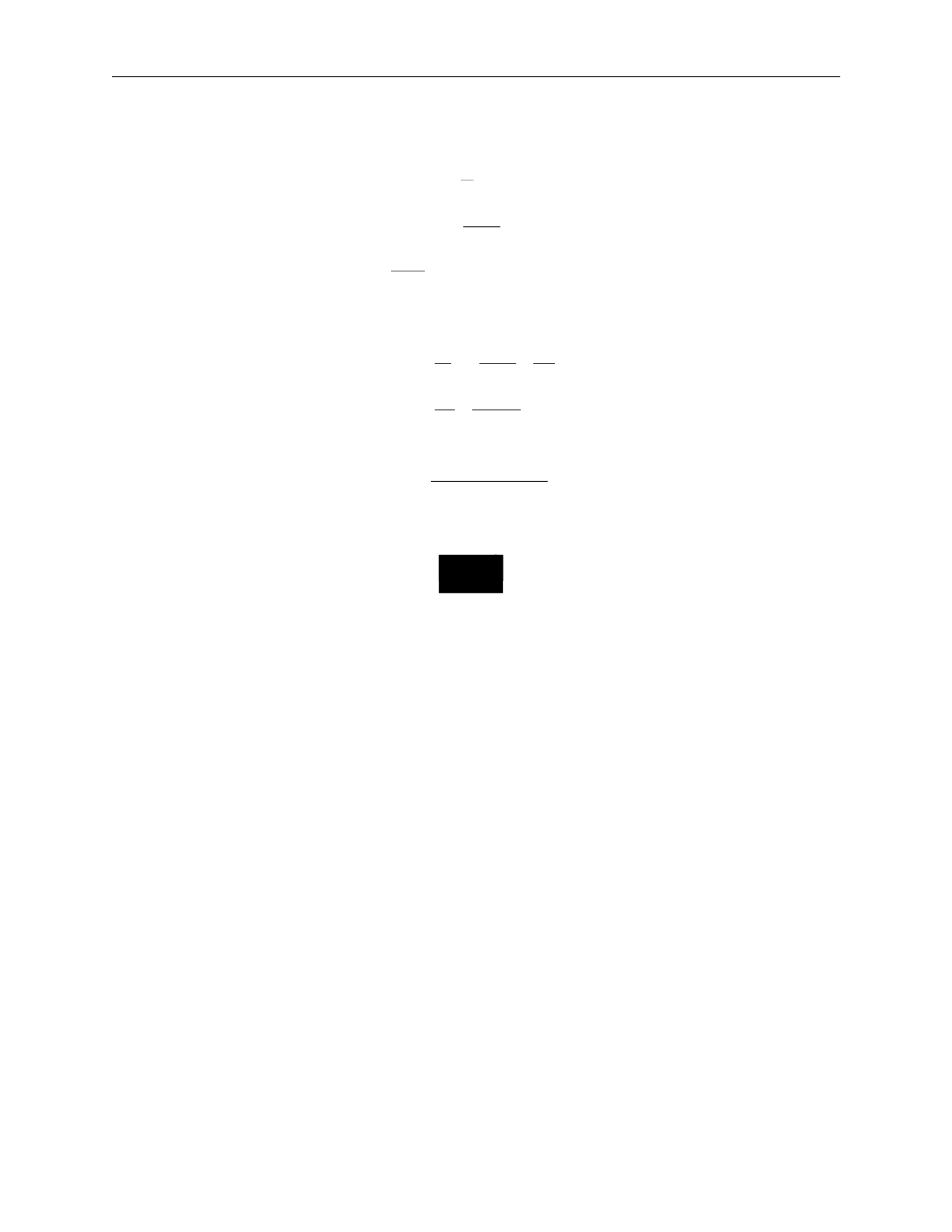
We can relate properties of a galaxy to observables through several equations:
R
θ
=
(apparent size)
d
L
F
=
4πd
2
(158)
v
2
=
GM .
R
Introducing surface brightness Σ
F
L
d
2
Σ =
=
θ
2
4πd
2
R
2
(159)
L
v
4
then
=
4π
·
G2M 2
v
4
L =
Σ4πG
2
(M/L)
2
.
(160)
If we assume, for a given class of galaxies, that the surface brightness and the mass-to-light
ratio are the same, then
.
(161)
This introduces two important relations.
The Tully-Fischer relation is used for spiral galaxies and relates the maximum velocity in
the rotation curve
v
max
, which can be measured from HII spectra, and the luminosity:
4
max
.
(162)
The Faber-Jackson relation is used for ellipticals and relates the velocity dispersion
σ
v
to the
luminosity:
L
∝
σ
4
.
(163)
Thus, we can get an estimate of the intrinsic luminosity of a galaxy be measuring stel-
lar velocities. The constant of proportionality is roughly
L
∗
/(220 km/s)
4
, where
L
∗
is the
characteristic galaxy luminosity.
3.D
Phase-space distribution function
We have described the individual orbits in a potential, but this is not sufficient to describe
galactic dynamics. We want information of the configuration of all particles. Each star is
described by its position
→
x
and velocity
→
v
,
and we need to know this for all stars, i.e. how
stars are distributed in the 6D phase space
(
→
x
,
→
v
)
.
We define a phase-space distribution function
f
(
→
x
,
→
v
,
t)d3
→
x
d
3
→
v
(164)
∝
L
∝
v
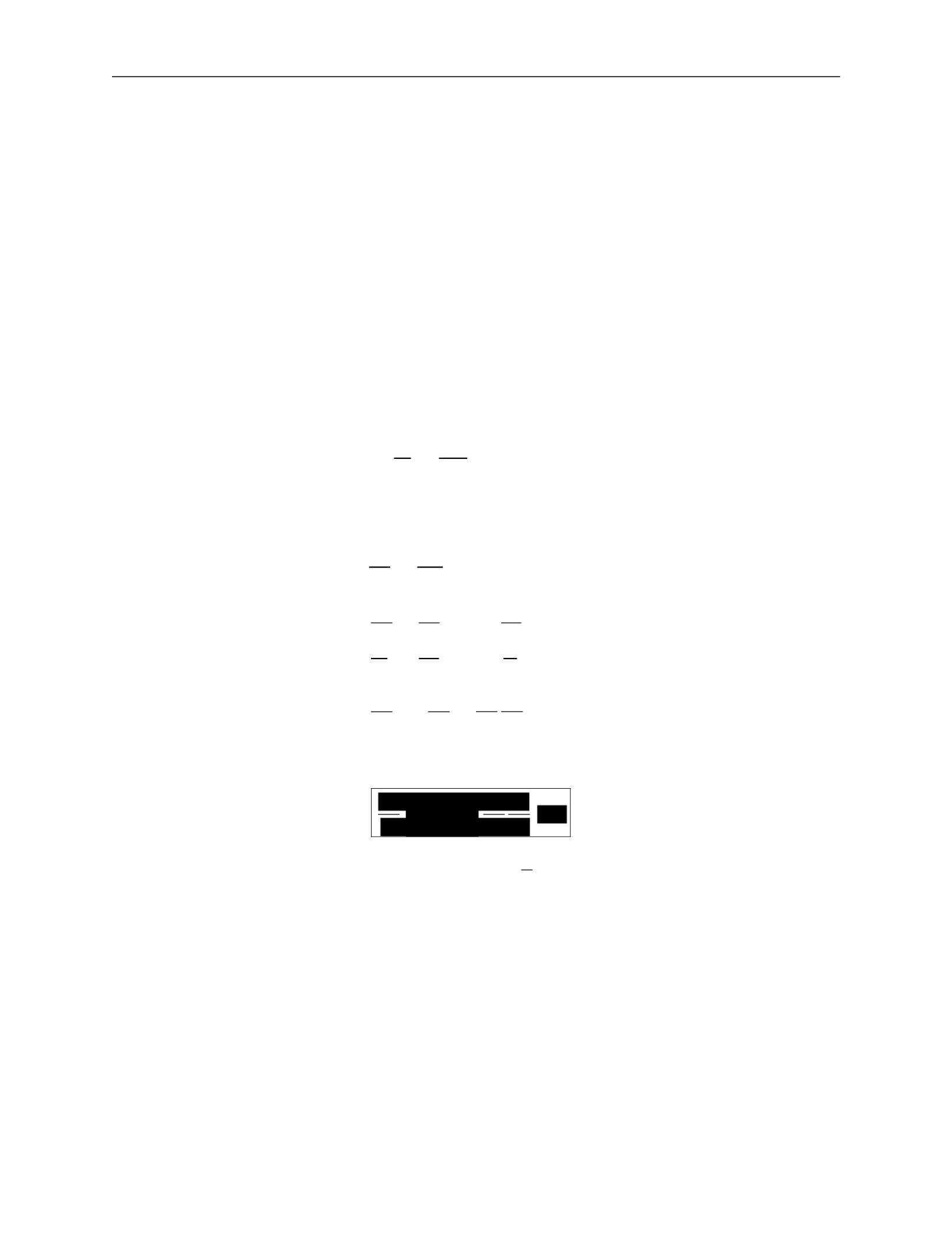
3.
MODELLING GALAXIES
39
∈
dt
as the probability that at time
t
, a randomly chosen star has
(
→
x
∗
,
→
v
∗
)
([
→
x
,
→
x
+
d
→
x
]
,
[
→
v
,
→
v
+
d
→
v])
.
This
means
that
the function must be normalized for all
t
, i.e.
∫
f
(
→
x
,
→
v
,
t)d
3
→
x
d
3
→
v
= 1 .
(165)
Collisionless
Boltzmann
equation
:
We want to describe the time evolution of
f
(
→
x
,
→
v
,
t)
. Since probability cannot be destroyed,
the 6D continuity equation must hold.
We define the 6D phase-space vector
then
w
→
=
(
→
x
,
→
v
)
(166)
∂f
+
∂
f
w
→
˙
=
0 .
(167)
∂t
∂w
→
This is the same form as the standard 3D continuity equation. We can rewrite this by
expanding out
w
→
and using velocity
→
v
=
→
x
˙
and acceleration
→
a
=
→
v
˙
:
0
= ∂f +
∂
f
w
→
˙
∂t
∂w
→
∂f
∂
=
+
∂t
∂
→
x
(
f
→
x
˙
) +
∂
(
f
→
v
˙
)
∂
→
v
(168)
∂f
∂
∂
=
+
(
f
→
v
)
+
f
(
−
∇
→
φ)
∂t
∂
→
x
∂
→
v
∂f
∂f
∂φ
∂f
=
∂t
+
→
v
∂
→
x
−
∂
→
x
∂
→
v
.
This gives us the collisionless Boltzmann equation (CBE):
.
(169)
Note that another way to see this is by writing out
df
= 0
and taking the limits
lim
→x
→∞
= 0
and
lim
→v
→∞
= 0
.
General Jeans equations:
A solution to the collisionless Boltzmann equation is difficult to obtain, so we instead study
moments of the CBE and the phase-space distribution.
Moments of the phase-space density give us some average quantities of the system.
a)
The first moment gives the density
n
of the system:
n
=
∫
f
d
3
→
v
.
(170)
∂t
−
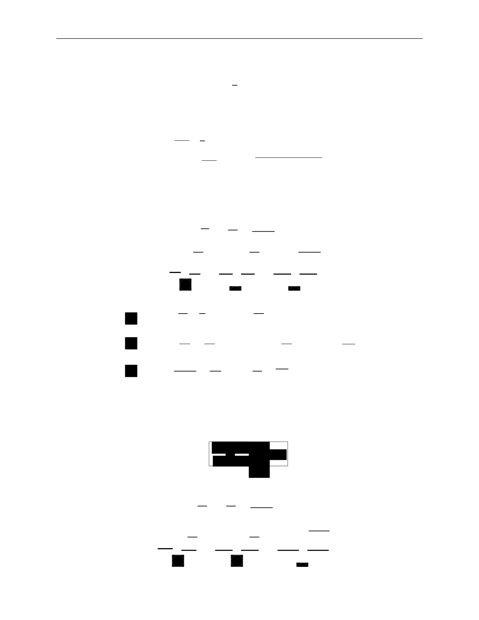
3.
MODELLING GALAXIES
40
ij
∫
—
∫
∫
∫
±∞
—
i
n
i
i
j
n
i
j
∂
→
x
∂
→
v
∂
→
x
∂
→
v
∂
→
x
→v=
−∞
j
∂t
j
∂
→
x
j
∂
→
x
∂
→
v
2
b)
The second moment gives the average velocity
v
¯
i
:
v
¯
=
1
∫
v
f
d
3
→
v
.
(171)
c)
The third moment gives the velocity dispersion
σ
2
:
v v
=
1
∫
v v
f
d
3
→
v
ij
=
v
i
v
j
−
v
¯
i
v
¯
j
=
(v
i
−
v
¯
i
)(
v
j
−
v
¯
j
)
.
We now examine moments of the collisionless Boltzmann equation more closely. We break
each integral into three terms to simplify each individually.
c)
First moment:
d
3
→
v
∂f
∂t
∂f
+
→
v
∂
→
x
∂φ
∂f
=
0
∂
→
x
∂
→
v
∫
d
3
→
v
∂f +
∫
d
3
→
v
→
v
∂f
−
∫
d
3
→
v
∂φ
∂f =
0 (173)
∂t
` ˛
1
¸ x
∂
→
x
` ˛
2
¸ x
∂
→
x
∂
→
v
` ˛
3
¸ x
:
d
3
→
v
∂f =
∂
∂t ∂t
d
3
→
v
f
=
∂n
∂t
:
d
3
→
v
→
v
∂f
∂
→
x
∂
=
∂
→
x
d3
→
v
→
v
f
=
∂
∂
→
x
n
→
v
¯
=
Σ
∂
∂x
i
(
n
v
¯
i
)
(174)
:
∫
d
3
→
v
∂φ
∂f
=
∂φ
∫
d
3
→
v
∂f
=
∂φ [f ]
→v=+
∞
=
0
For the third term, we used the fact that phase-space distribution goes to 0 at
for
physical systems.
This gives us the 3D continuity equation:
d)
Second moment:
.
(175)
∫
d
3
→
v
vj
∂f
∂f
+
→
v
∂t
∂
→
x
∂φ
∂f
=
0
∂
→
x
∂
→
v
∫
d
3
→
v
v
∂f +
∫
d
3
→
v
v
→
v
∂f
−
∫
d
3
→
v
v
∂φ
∂f
=
0
(176)
` ˛
1
¸ x ` ˛
2
¸ x ` ˛
3
¸ x
1
2
3
∂n ∂
∂t
0
σ
∫
i
(172)

3.
MODELLING GALAXIES
41
ij
Σ
∫
i
∂x
∂x
j
∂t
∂t
j
∂t
j
∂t
∂t
∂x
i
∂t
∂t
j
∂x
i
using the continuity equation ∂n
=
−
Σ
∂
(
n
v
¯
)
j
∂
→
x
i
∂x
i
∂x
i
j
i
i
∂x
ij
i
j
∂x
j
∂v
j
v
i
=
−∞
i
∂v
∂t
∂x
i
∂x
ij
i
j
∂x
i
`
i
i
ij
i
∂x
i
∂v
:
∫
d
3
→
v
v
∂f =
∂
∫
d
3
→
v
v
f =
∂
(
n
v
¯
) =
∂
n
v
¯
+
n
∂
v
¯
j
=
−
v
¯
Σ
∂
(
n
v
¯
) +
n
∂
v
¯
j
=
n
∂
v
¯
j
−
v
¯
Σ
∂
(
n
v
¯
)
∂t
∂x
i
i
to go from the first line to the second
:
∫
d
3
→
v
v
→
v
∂f
=
∫
d
3
→
v
v
Σ
v
∂f =
Σ
∂
∫
d
3
→
v
v v
f
= nv
j
v
i
`
= n
˛ ¸
σ
2
+
x
v
¯
i
v
¯
j
=
Σ
∂
n
σ
2
+
v
¯
v
¯
:
∫
d
3
→
v
v
∂φ
∂f
=
∫
d
3
→
v
v
Σ
∂φ
∂f
=
Σ
∂φ
∫
d
3
→
v
v
∂f
(177)
((k, l, i) are permutations of (1, 2, 3))
=
∂φ
dv
∂x
k
∫
dv
l
∫
dv
i
∂f
v
j
∂v
=
[v
f
]
˛
v
¸
i
=+
∞
−
x
∫
dv ∂v
j
f
= 0
−
∫
dv
i
δ
ij
f
=
−
Σ
∂φ
∫
dv
∫
dv
l
∫
dv
i
δ
ij
f
i
i
=
−
Σ
∂φ
∫
d
3
→
v
δ
f
i
i
∂φ
=
−
n∂x
j
Plugging each term back in, we get
n
∂
v
¯
j
−
v
¯
Σ
∂
(
n
v
¯
) +
Σ
∂
n
σ
2
+
v
¯
v
¯
+
n
∂φ
=
0
(178)
i
i
i
i
i
i
i
i
i
i
i
1
2
3
j
j
i
j
i
i
j
∂
→
x
∂
→
v
j
i
i
i
j
k

3.
MODELLING GALAXIES
42
Σ
v
¯
2
2
∂t
j
∂x
i
∂x
ij
i
∂x
i
i
j
∂x
j
=
(
n
v
¯
i
)
∂
x
v
¯
j
+
v
¯
j
∂x
(
n
v
¯
i
)
∂t
i
∂x
j
∂x
ij
∂x
—
1
Σ
∂(nσ
ij
) :
pressure
∂t
i
i
i
i
i
i
i
i
j
which we can rewrite
n
∂
v
¯
j
−
v
¯
Σ
∂
(
n
v
¯
)
+
Σ
∂
(nσ
2
)+
Σ
∂
(
n
v
¯
v
¯
)
+n
∂φ
=
0
`
Σ˛¸
∂
x
Σ
∂
(179)
where the two underlined terms cancel. This gives us
n
∂
v
¯
j
+
Σ
(
n
v
¯
)
∂
v
¯
+
Σ
∂
(nσ
2
) +
n
∂φ
=
0 .
(180)
This is the Jeans equation, often written
(181)
Each term can be physically interpreted:
∂
v
¯
j
∂t
∂
v
¯
j
i
∂x
: acceleration of fluid
: kinematic viscosity/shear
i
i
2
(182)
n
∂x
i
∂φ
−
∂x
j
: gravity
Jeans
equations
in
spherical
systems
:
We can convert to spherical coordinates and take velocity moments to give us the Jeans
equations in spherical coordinates. This is complicated!
To simplify, we take the radial Jeans equation and focus on steady-state symmetric systems.
Implications:
∂
=
0
since we have steady state
•
v
¯
r
=
0
otherwise we have net radial motion
•
v
¯
θ
=
v
¯
φ
=
0
or the symmetry is broken
•
σ
rφ
=
0
or the symmetry is broken
2
•
σ
φφ
≡
σ
or the symmetry is broken.
2
2
rθ
θθ
t
∂φ
1
∂t
•
=
σ
=
σ
i
i
i
i
i
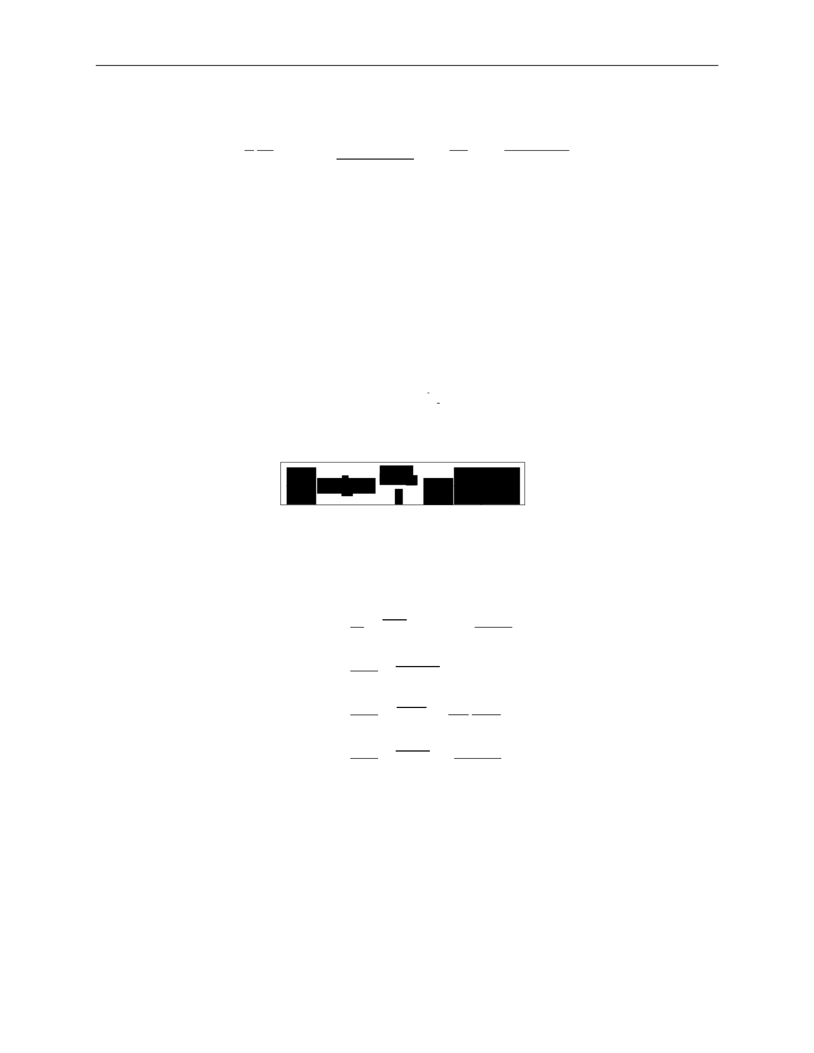
3.
MODELLING GALAXIES
43
2
2
2
2
t
t
t
— t
2
rr
rσ
rσ
rσ
rr
r
∂r
G
n
∂r
rr
—
dr
2
—
The simplified Jeans equation is:
1 ∂ 2(σ2
− σ ) ∂φ
GM (< r)
(nσ
2
) +
rr
t
=
−
=
−
(183)
where we’ve plugged in gravity as the force.
We have three limits we can look at:
•
σ
rr
•
σ
rr
•
σ
rr
σ
2
: nearly circular orbits
σ
2
: nearly radial orbits
= σ
2
: isotropic orbits
We define the anisotropy parameter:
σ
2
β
=
1
rr
(184)
which gives us a useful form of the Jeans equation for observations:
.
(185)
This depends only on radial components with uncertainty from
β
, assuming spherical sym-
metry and a steady-state system.
This can be simplified further to get mass estimates:
r2
1 ∂ 2 2βσ2
M (< r)
=
−
(nσ
)
+
2
=
−
rr
r
∂
(nσ
2
)
+
2β
G
2
=
rr
G
2
rr
r dn
+
n dr
rr
r
dσ
2
rr
+
2β
rr
(186)
2
=
rr
G
d ln n
+
d ln r
d ln σ2
rr
+
2β
d ln r
where the last line can be measured with observations.
Stability of stellar systems
The existence of equilibrium solutions to the collisionless Boltzmann equation does not assure
stability. Real stellar systems are subject to perturbations. What is important for stability?
1 ∂
2βσ2
σ
nσ
σ
n
∂r
r
2
r
∂r
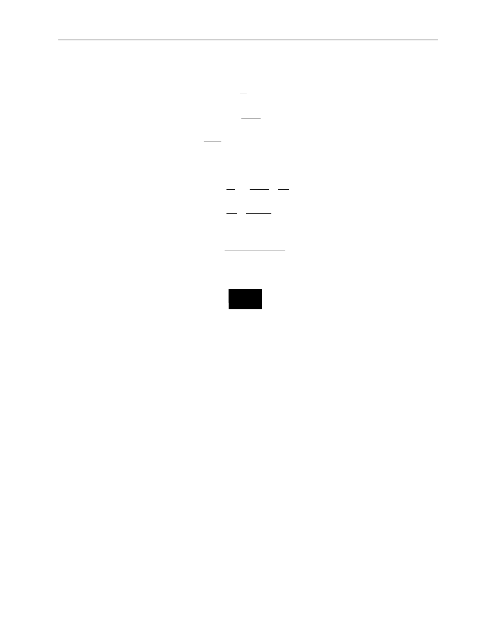
3.
MODELLING GALAXIES
38
v
·
Luminosity-velocity relations:
We can relate properties of a galaxy to observables through several equations:
R
θ
=
(apparent size)
d
L
F
=
4πd
2
(158)
v
2
=
GM .
R
Introducing surface brightness Σ
F
L
d
2
Σ =
=
θ
2
4πd
2
R
2
(159)
L
v
4
then
=
4π
·
G2M 2
v
4
L =
Σ4πG
2
(M/L)
2
.
(160)
If we assume, for a given class of galaxies, that the surface brightness and the mass-to-light
ratio are the same, then
.
(161)
This introduces two important relations.
The Tully-Fischer relation is used for spiral galaxies and relates the maximum velocity in
the rotation curve
v
max
, which can be measured from HII spectra, and the luminosity:
4
max
.
(162)
The Faber-Jackson relation is used for ellipticals and relates the velocity dispersion
σ
v
to the
luminosity:
L
∝
σ
4
.
(163)
Thus, we can get an estimate of the intrinsic luminosity of a galaxy be measuring stel-
lar velocities. The constant of proportionality is roughly
L
∗
/(220 km/s)
4
, where
L
∗
is the
characteristic galaxy luminosity.
3.E
Phase-space distribution function
We have described the individual orbits in a potential, but this is not sufficient to describe
galactic dynamics. We want information of the configuration of all particles. Each star is
described by its position
→
x
and velocity
→
v
,
and we need to know this for all stars, i.e. how
stars are distributed in the 6D phase space
(
→
x
,
→
v
)
.
We define a phase-space distribution function
f
(
→
x
,
→
v
,
t)d3
→
x
d
3
→
v
(164)
∝
L
∝
v

3.
MODELLING GALAXIES
39
∈
dt
as the probability that at time
t
, a randomly chosen star has
(
→
x
∗
,
→
v
∗
)
([
→
x
,
→
x
+
d
→
x
]
,
[
→
v
,
→
v
+
d
→
v])
.
This
means
that
the function must be normalized for all
t
, i.e.
∫
f
(
→
x
,
→
v
,
t)d
3
→
x
d
3
→
v
= 1 .
(165)
Collisionless
Boltzmann
equation
:
We want to describe the time evolution of
f
(
→
x
,
→
v
,
t)
. Since probability cannot be destroyed,
the 6D continuity equation must hold.
We define the 6D phase-space vector
then
w
→
=
(
→
x
,
→
v
)
(166)
∂f
+
∂
f
w
→
˙
=
0 .
(167)
∂t
∂w
→
This is the same form as the standard 3D continuity equation. We can rewrite this by
expanding out
w
→
and using velocity
→
v
=
→
x
˙
and acceleration
→
a
=
→
v
˙
:
0
= ∂f +
∂
f
w
→
˙
∂t
∂w
→
∂f
∂
=
+
∂t
∂
→
x
(
f
→
x
˙
) +
∂
(
f
→
v
˙
)
∂
→
v
(168)
∂f
∂
∂
=
+
(
f
→
v
)
+
f
(
−
∇
→
φ)
∂t
∂
→
x
∂
→
v
∂f
∂f
∂φ
∂f
=
∂t
+
→
v
∂
→
x
−
∂
→
x
∂
→
v
.
This gives us the collisionless Boltzmann equation (CBE):
.
(169)
Note that another way to see this is by writing out
df
= 0
and taking the limits
lim
→x
→∞
= 0
and
lim
→v
→∞
= 0
.
General Jeans equations:
A solution to the collisionless Boltzmann equation is difficult to obtain, so we instead study
moments of the CBE and the phase-space distribution.
Moments of the phase-space density give us some average quantities of the system.
a)
The first moment gives the density
n
of the system:
n
=
∫
f
d
3
→
v
.
(170)
∂t
−
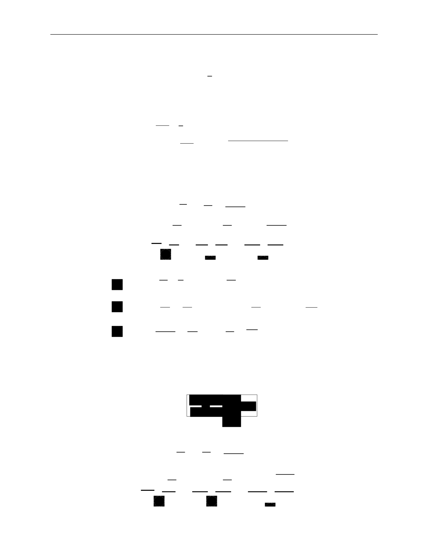
3.
MODELLING GALAXIES
40
ij
∫
—
∫
∫
∫
±∞
—
i
n
i
i
j
n
i
j
∂
→
x
∂
→
v
∂
→
x
∂
→
v
∂
→
x
→v=
−∞
j
∂t
j
∂
→
x
j
∂
→
x
∂
→
v
2
b)
The second moment gives the average velocity
v
¯
i
:
v
¯
=
1
∫
v
f
d
3
→
v
.
(171)
c)
The third moment gives the velocity dispersion
σ
2
:
v v
=
1
∫
v v
f
d
3
→
v
ij
=
v
i
v
j
−
v
¯
i
v
¯
j
=
(v
i
−
v
¯
i
)(
v
j
−
v
¯
j
)
.
We now examine moments of the collisionless Boltzmann equation more closely. We break
each integral into three terms to simplify each individually.
e)
First moment:
d
3
→
v
∂f
∂t
∂f
+
→
v
∂
→
x
∂φ
∂f
=
0
∂
→
x
∂
→
v
∫
d
3
→
v
∂f +
∫
d
3
→
v
→
v
∂f
−
∫
d
3
→
v
∂φ
∂f =
0 (173)
∂t
` ˛
1
¸ x
∂
→
x
` ˛
2
¸ x
∂
→
x
∂
→
v
` ˛
3
¸ x
:
d
3
→
v
∂f =
∂
∂t ∂t
d
3
→
v
f
=
∂n
∂t
:
d
3
→
v
→
v
∂f
∂
→
x
∂
=
∂
→
x
d3
→
v
→
v
f
=
∂
∂
→
x
n
→
v
¯
=
Σ
∂
∂x
i
(
n
v
¯
i
)
(174)
:
∫
d
3
→
v
∂φ
∂f
=
∂φ
∫
d
3
→
v
∂f
=
∂φ [f ]
→v=+
∞
=
0
For the third term, we used the fact that phase-space distribution goes to 0 at
for
physical systems.
This gives us the 3D continuity equation:
f)
Second moment:
.
(175)
∫
d
3
→
v
vj
∂f
∂f
+
→
v
∂t
∂
→
x
∂φ
∂f
=
0
∂
→
x
∂
→
v
∫
d
3
→
v
v
∂f +
∫
d
3
→
v
v
→
v
∂f
−
∫
d
3
→
v
v
∂φ
∂f
=
0
(176)
` ˛
1
¸ x ` ˛
2
¸ x ` ˛
3
¸ x
1
2
3
∂n ∂
∂t
0
σ
∫
i
(172)

3.
MODELLING GALAXIES
41
ij
Σ
∫
i
∂x
∂x
j
∂t
∂t
j
∂t
j
∂t
∂t
∂x
i
∂t
∂t
j
∂x
i
using the continuity equation ∂n
=
−
Σ
∂
(
n
v
¯
)
j
∂
→
x
i
∂x
i
∂x
i
j
i
i
∂x
ij
i
j
∂x
j
∂v
j
v
i
=
−∞
i
∂v
∂t
∂x
i
∂x
ij
i
j
∂x
i
`
i
i
ij
i
∂x
i
∂v
:
∫
d
3
→
v
v
∂f =
∂
∫
d
3
→
v
v
f =
∂
(
n
v
¯
) =
∂
n
v
¯
+
n
∂
v
¯
j
=
−
v
¯
Σ
∂
(
n
v
¯
) +
n
∂
v
¯
j
=
n
∂
v
¯
j
−
v
¯
Σ
∂
(
n
v
¯
)
∂t
∂x
i
i
to go from the first line to the second
:
∫
d
3
→
v
v
→
v
∂f
=
∫
d
3
→
v
v
Σ
v
∂f =
Σ
∂
∫
d
3
→
v
v v
f
= nv
j
v
i
`
= n
˛ ¸
σ
2
+
x
v
¯
i
v
¯
j
=
Σ
∂
n
σ
2
+
v
¯
v
¯
:
∫
d
3
→
v
v
∂φ
∂f
=
∫
d
3
→
v
v
Σ
∂φ
∂f
=
Σ
∂φ
∫
d
3
→
v
v
∂f
(177)
((k, l, i) are permutations of (1, 2, 3))
=
∂φ
dv
∂x
k
∫
dv
l
∫
dv
i
∂f
v
j
∂v
=
[v
f
]
˛
v
¸
i
=+
∞
−
x
∫
dv ∂v
j
f
= 0
−
∫
dv
i
δ
ij
f
=
−
Σ
∂φ
∫
dv
∫
dv
l
∫
dv
i
δ
ij
f
i
i
=
−
Σ
∂φ
∫
d
3
→
v
δ
f
i
i
∂φ
=
−
n∂x
j
Plugging each term back in, we get
n
∂
v
¯
j
−
v
¯
Σ
∂
(
n
v
¯
) +
Σ
∂
n
σ
2
+
v
¯
v
¯
+
n
∂φ
=
0
(178)
i
i
i
i
i
i
i
i
i
i
i
1
2
3
j
j
i
j
i
i
j
∂
→
x
∂
→
v
j
i
i
i
j
k

3.
MODELLING GALAXIES
42
Σ
v
¯
2
2
∂t
j
∂x
i
∂x
ij
i
∂x
i
i
j
∂x
j
=
(
n
v
¯
i
)
∂
x
v
¯
j
+
v
¯
j
∂x
(
n
v
¯
i
)
∂t
i
∂x
j
∂x
ij
∂x
—
1
Σ
∂(nσ
ij
) :
pressure
∂t
i
i
i
i
i
i
i
i
j
which we can rewrite
n
∂
v
¯
j
−
v
¯
Σ
∂
(
n
v
¯
)
+
Σ
∂
(nσ
2
)+
Σ
∂
(
n
v
¯
v
¯
)
+n
∂φ
=
0
`
Σ˛¸
∂
x
Σ
∂
(179)
where the two underlined terms cancel. This gives us
n
∂
v
¯
j
+
Σ
(
n
v
¯
)
∂
v
¯
+
Σ
∂
(nσ
2
) +
n
∂φ
=
0 .
(180)
This is the Jeans equation, often written
(181)
Each term can be physically interpreted:
∂
v
¯
j
∂t
∂
v
¯
j
i
∂x
: acceleration of fluid
: kinematic viscosity/shear
i
i
2
(182)
n
∂x
i
∂φ
−
∂x
j
: gravity
Jeans
equations
in
spherical
systems
:
We can convert to spherical coordinates and take velocity moments to give us the Jeans
equations in spherical coordinates. This is complicated!
To simplify, we take the radial Jeans equation and focus on steady-state symmetric systems.
Implications:
∂
=
0
since we have steady state
•
v
¯
r
=
0
otherwise we have net radial motion
•
v
¯
θ
=
v
¯
φ
=
0
or the symmetry is broken
•
σ
rφ
=
0
or the symmetry is broken
2
•
σ
φφ
≡
σ
or the symmetry is broken.
2
2
rθ
θθ
t
∂φ
1
∂t
•
=
σ
=
σ
i
i
i
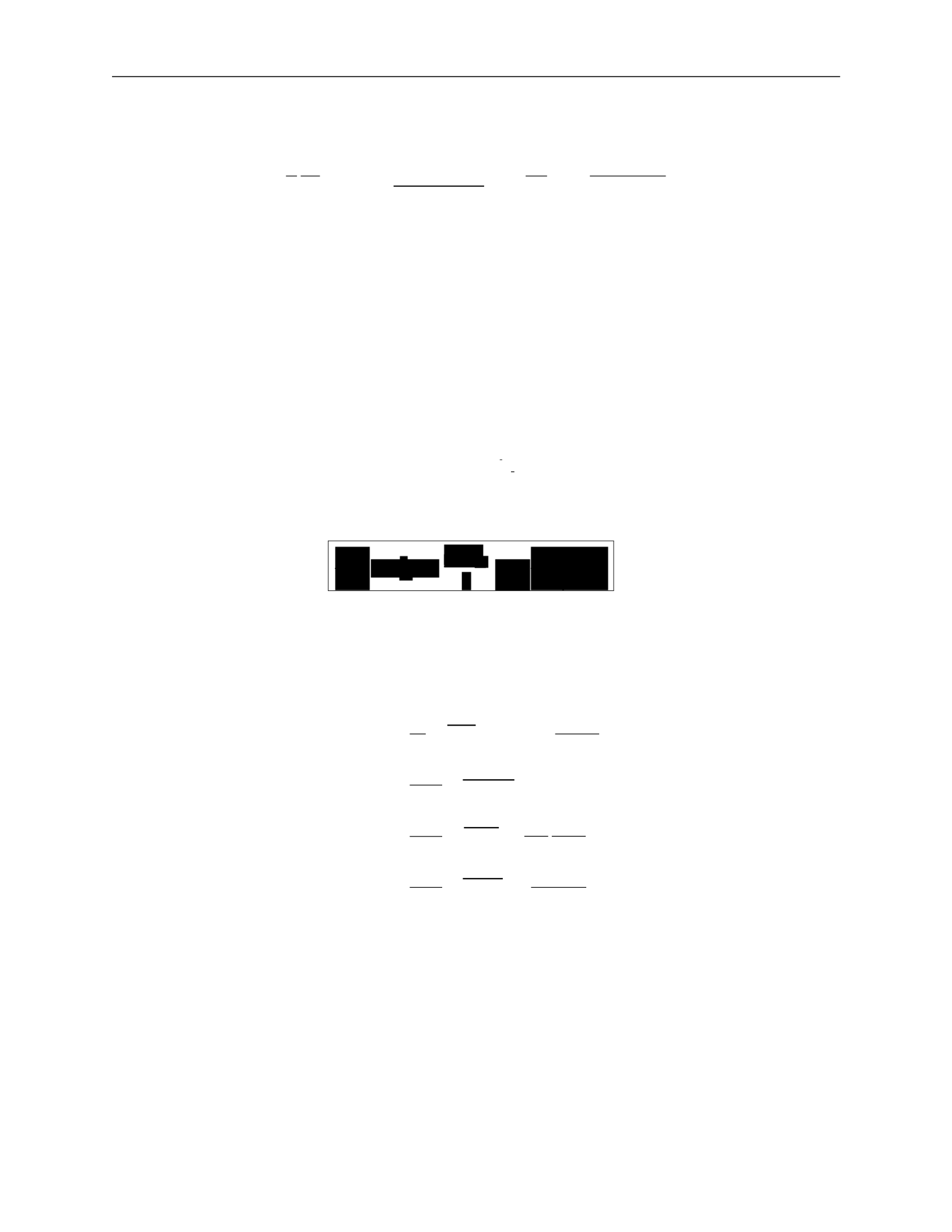
i
i
3.
MODELLING GALAXIES
43
2
2
2
2
t
t
t
— t
2
rr
rσ
rσ
rσ
rr
r
∂r
G
n
∂r
rr
—
dr
2
—
The simplified Jeans equation is:
1 ∂ 2(σ2
− σ ) ∂φ
GM (< r)
(nσ
2
) +
rr
t
=
−
=
−
(183)
where we’ve plugged in gravity as the force.
We have three limits we can look at:
•
σ
rr
•
σ
rr
•
σ
rr
σ
2
: nearly circular orbits
σ
2
: nearly radial orbits
= σ
2
: isotropic orbits
We define the anisotropy parameter:
σ
2
β
=
1
rr
(184)
which gives us a useful form of the Jeans equation for observations:
.
(185)
This depends only on radial components with uncertainty from
β
, assuming spherical sym-
metry and a steady-state system.
This can be simplified further to get mass estimates:
r2
1 ∂ 2 2βσ2
M (< r)
=
−
(nσ
)
+
2
=
−
rr
r
∂
(nσ
2
)
+
2β
G
2
=
rr
G
2
rr
r dn
+
n dr
rr
r
dσ
2
rr
+
2β
rr
(186)
2
=
rr
G
d ln n
+
d ln r
d ln σ2
rr
+
2β
d ln r
where the last line can be measured with observations.
Stability of stellar systems
The existence of equilibrium solutions to the collisionless Boltzmann equation does not assure stability.
Real stellar systems are subject to perturbations. What is important for stability?
1 ∂
2βσ2
σ
nσ
σ
n
∂r
r
2
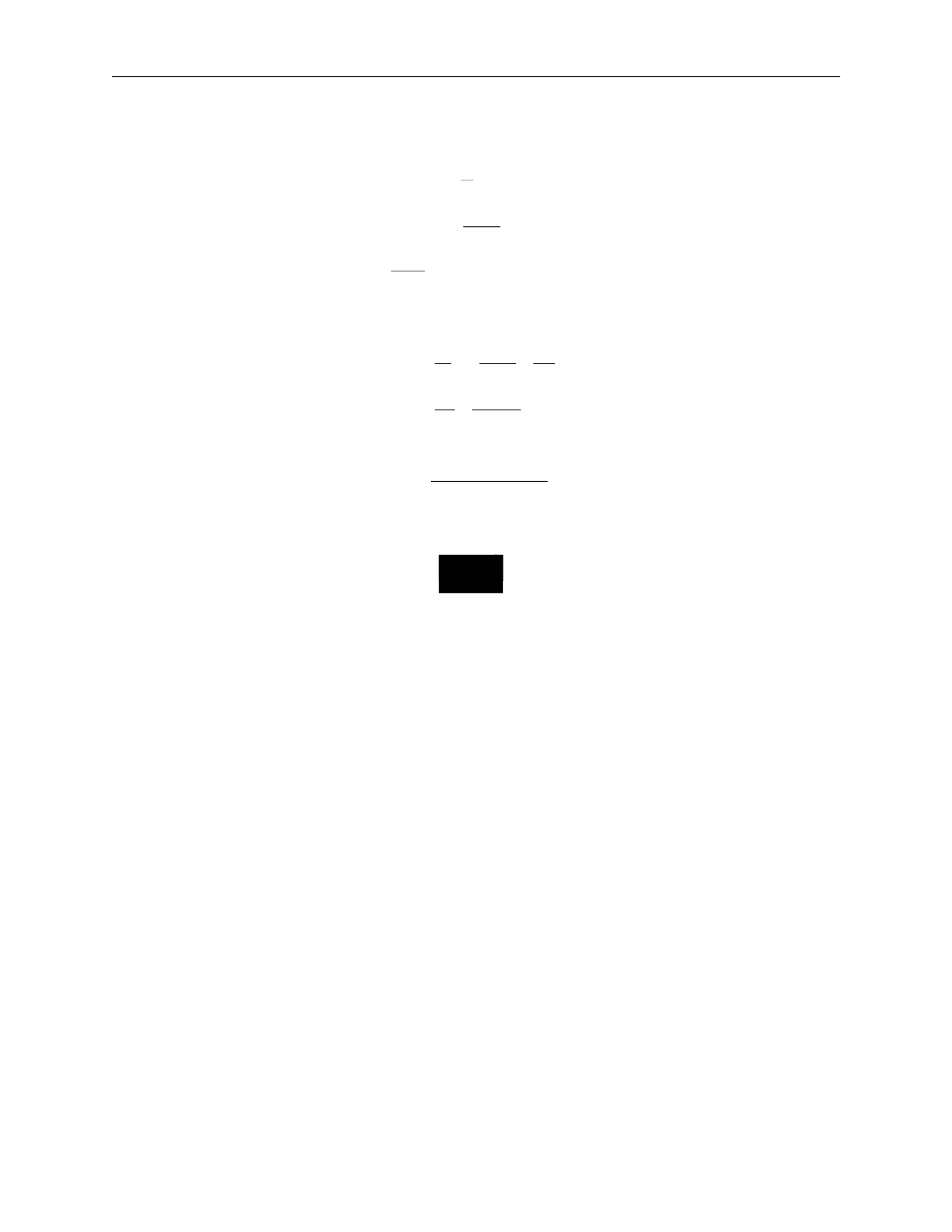
r
∂r
3.
MODELLING GALAXIES
38
v
·
Luminosity-velocity relations:
We can relate properties of a galaxy to observables through several equations:
R
θ
=
(apparent size)
d
L
F
=
4πd
2
(158)
v
2
=
GM .
R
Introducing surface brightness Σ
F
L
d
2
Σ =
=
θ
2
4πd
2
R
2
(159)
L
v
4
then
=
4π
·
G2M 2
v
4
L =
Σ4πG
2
(M/L)
2
.
(160)
If we assume, for a given class of galaxies, that the surface brightness and the mass-to-light
ratio are the same, then
.
(161)
This introduces two important relations.
The Tully-Fischer relation is used for spiral galaxies and relates the maximum velocity in
the rotation curve
v
max
, which can be measured from HII spectra, and the luminosity:
4
max
.
(162)
The Faber-Jackson relation is used for ellipticals and relates the velocity dispersion
σ
v
to the
luminosity:
L
∝
σ
4
.
(163)
Thus, we can get an estimate of the intrinsic luminosity of a galaxy be measuring stel-
lar velocities. The constant of proportionality is roughly
L
∗
/(220 km/s)
4
, where
L
∗
is the
characteristic galaxy luminosity.
3.F
Phase-space distribution function
We have described the individual orbits in a potential, but this is not sufficient to describe
galactic dynamics. We want information of the configuration of all particles. Each star is
described by its position
→
x
and velocity
→
v
,
and we need to know this for all stars, i.e. how
stars are distributed in the 6D phase space
(
→
x
,
→
v
)
.
We define a phase-space distribution function
f
(
→
x
,
→
v
,
t)d3
→
x
d
3
→
v
(164)
∝
L
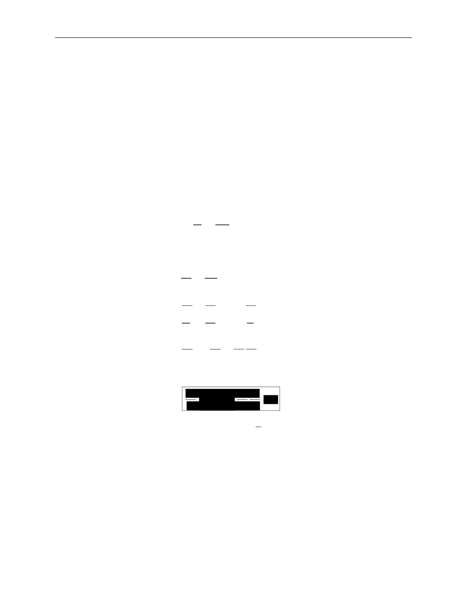
∝
v
3.
MODELLING GALAXIES
39
∈
dt
as the probability that at time
t
, a randomly chosen star has
(
→
x
∗
,
→
v
∗
)
([
→
x
,
→
x
+
d
→
x
]
,
[
→
v
,
→
v
+
d
→
v])
.
This
means
that
the function must be normalized for all
t
, i.e.
∫
f
(
→
x
,
→
v
,
t)d
3
→
x
d
3
→
v
= 1 .
(165)
Collisionless
Boltzmann
equation
:
We want to describe the time evolution of
f
(
→
x
,
→
v
,
t)
. Since probability cannot be destroyed,
the 6D continuity equation must hold.
We define the 6D phase-space vector
then
w
→
=
(
→
x
,
→
v
)
(166)
∂f
+
∂
f
w
→
˙
=
0 .
(167)
∂t
∂w
→
This is the same form as the standard 3D continuity equation. We can rewrite this by
expanding out
w
→
and using velocity
→
v
=
→
x
˙
and acceleration
→
a
=
→
v
˙
:
0
= ∂f +
∂
f
w
→
˙
∂t
∂w
→
∂f
∂
=
+
∂t
∂
→
x
(
f
→
x
˙
) +
∂
(
f
→
v
˙
)
∂
→
v
(168)
∂f
∂
∂
=
+
(
f
→
v
)
+
f
(
−
∇
→
φ)
∂t
∂
→
x
∂
→
v
∂f
∂f
∂φ
∂f
=
∂t
+
→
v
∂
→
x
−
∂
→
x
∂
→
v
.
This gives us the collisionless Boltzmann equation (CBE):
.
(169)
Note that another way to see this is by writing out
df
= 0
and taking the limits
lim
→x
→∞
= 0
and
lim
→v
→∞
= 0
.
General Jeans equations:
A solution to the collisionless Boltzmann equation is difficult to obtain, so we instead study
moments of the CBE and the phase-space distribution.
Moments of the phase-space density give us some average quantities of the system.
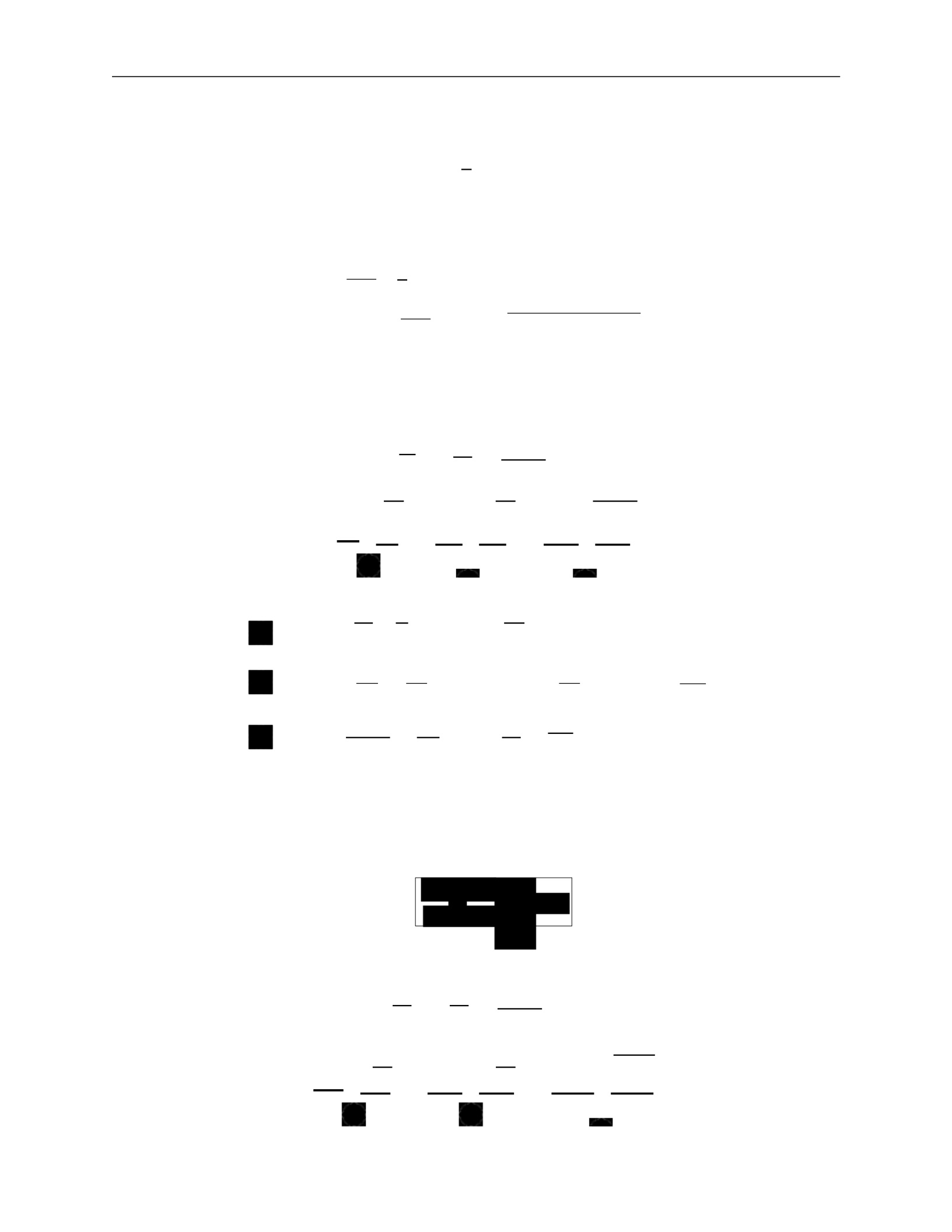
a)
The first moment gives the density
n
of the system:
n
=
∫
f
d
3
→
v
.
(170)
∂t
−
3.
MODELLING GALAXIES
40
ij
∫
—
∫
∫
∫
±∞
—
i
n
i
i
j
n
i
j
∂
→
x
∂
→
v
∂
→
x
∂
→
v
∂
→
x
→v=
−∞
j
∂t
j
∂
→
x
j
∂
→
x
∂
→
v
2
b)
The second moment gives the average velocity
v
¯
i
:
v
¯
=
1
∫
v
f
d
3
→
v
.
(171)
c)
The third moment gives the velocity dispersion
σ
2
:
v v
=
1
∫
v v
f
d
3
→
v
ij
=
v
i
v
j
−
v
¯
i
v
¯
j
=
(v
i
−
v
¯
i
)(
v
j
−
v
¯
j
)
.
We now examine moments of the collisionless Boltzmann equation more closely. We break
each integral into three terms to simplify each individually.
g)
First moment:
d
3
→
v
∂f
∂t
∂f
+
→
v
∂
→
x
∂φ
∂f
=
0
∂
→
x
∂
→
v
∫
d
3
→
v
∂f +
∫
d
3
→
v
→
v
∂f
−
∫
d
3
→
v
∂φ
∂f =
0 (173)
∂t
` ˛
1
¸ x
∂
→
x
` ˛
2
¸ x
∂
→
x
∂
→
v
` ˛
3
¸ x
:
d
3
→
v
∂f =
∂
∂t ∂t
d
3
→
v
f
=
∂n
∂t
:
d
3
→
v
→
v
∂f
∂
→
x
∂
=
∂
→
x
d3
→
v
→
v
f
=
∂
∂
→
x
n
→
v
¯
=
Σ
∂
∂x
i
(
n
v
¯
i
)
(174)
:
∫
d
3
→
v
∂φ
∂f
=
∂φ
∫
d
3
→
v
∂f
=
∂φ [f ]
→v=+
∞
=
0
For the third term, we used the fact that phase-space distribution goes to 0 at
for
physical systems.
This gives us the 3D continuity equation:
h)
Second moment:
.
(175)
∫
d
3
→
v
vj
∂f
∂f
+
→
v
∂t
∂
→
x
∂φ
∂f
=
0
∂
→
x
∂
→
v
∫
d
3
→
v
v
∂f +
∫
d
3
→
v
v
→
v
∂f
−
∫
d
3
→
v
v
∂φ
∂f
=
0
(176)
` ˛
1
¸ x ` ˛
2
¸ x ` ˛
3
¸ x
1
2
3
∂n ∂
∂t
0
σ
∫
i
(172)

3.
MODELLING GALAXIES
41
ij
Σ
∫
i
∂x
∂x
j
∂t
∂t
j
∂t
j
∂t
∂t
∂x
i
∂t
∂t
j
∂x
i
using the continuity equation ∂n
=
−
Σ
∂
(
n
v
¯
)
j
∂
→
x
i
∂x
i
∂x
i
j
i
i
∂x
ij
i
j
∂x
j
∂v
j
v
i
=
−∞
i
∂v
∂t
∂x
i
∂x
ij
i
j
∂x
i
`
i
i
ij
i
∂x
i
∂v
:
∫
d
3
→
v
v
∂f =
∂
∫
d
3
→
v
v
f =
∂
(
n
v
¯
) =
∂
n
v
¯
+
n
∂
v
¯
j
=
−
v
¯
Σ
∂
(
n
v
¯
) +
n
∂
v
¯
j
=
n
∂
v
¯
j
−
v
¯
Σ
∂
(
n
v
¯
)
∂t
∂x
i
i
to go from the first line to the second
:
∫
d
3
→
v
v
→
v
∂f
=
∫
d
3
→
v
v
Σ
v
∂f =
Σ
∂
∫
d
3
→
v
v v
f
= nv
j
v
i
`
= n
˛ ¸
σ
2
+
x
v
¯
i
v
¯
j
=
Σ
∂
n
σ
2
+
v
¯
v
¯
:
∫
d
3
→
v
v
∂φ
∂f
=
∫
d
3
→
v
v
Σ
∂φ
∂f
=
Σ
∂φ
∫
d
3
→
v
v
∂f
(177)
((k, l, i) are permutations of (1, 2, 3))
=
∂φ
dv
∂x
k
∫
dv
l
∫
dv
i
∂f
v
j
∂v
=
[v
f
]
˛
v
¸
i
=+
∞
−
x
∫
dv ∂v
j
f
= 0
−
∫
dv
i
δ
ij
f
=
−
Σ
∂φ
∫
dv
∫
dv
l
∫
dv
i
δ
ij
f
i
i
=
−
Σ
∂φ
∫
d
3
→
v
δ
f
i
i
∂φ
=
−
n∂x
j
Plugging each term back in, we get
n
∂
v
¯
j
−
v
¯
Σ
∂
(
n
v
¯
) +
Σ
∂
n
σ
2
+
v
¯
v
¯
+
n
∂φ
=
0
(178)
i
i
i
i
i
i
i
i
i
i
i
1
2
3
j
j
i
j
i
i
j
∂
→
x
∂
→
v
j
i
i
i
j
k

3.
MODELLING GALAXIES
42
Σ
v
¯
2
2
∂t
j
∂x
i
∂x
ij
i
∂x
i
i
j
∂x
j
=
(
n
v
¯
i
)
∂
x
v
¯
j
+
v
¯
j
∂x
(
n
v
¯
i
)
∂t
i
∂x
j
∂x
ij
∂x
—
1
Σ
∂(nσ
ij
) :
pressure
∂t
i
i
i
i
i
i
i
i
j
which we can rewrite
n
∂
v
¯
j
−
v
¯
Σ
∂
(
n
v
¯
)
+
Σ
∂
(nσ
2
)+
Σ
∂
(
n
v
¯
v
¯
)
+n
∂φ
=
0
`
Σ˛¸
∂
x
Σ
∂
(179)
where the two underlined terms cancel. This gives us
n
∂
v
¯
j
+
Σ
(
n
v
¯
)
∂
v
¯
+
Σ
∂
(nσ
2
) +
n
∂φ
=
0 .
(180)
This is the Jeans equation, often written
(181)
Each term can be physically interpreted:
∂
v
¯
j
∂t
∂
v
¯
j
i
∂x
: acceleration of fluid
: kinematic viscosity/shear
i
i
2
(182)
n
∂x
i
∂φ
−
∂x
j
: gravity
Jeans
equations
in
spherical
systems
:
We can convert to spherical coordinates and take velocity moments to give us the Jeans
equations in spherical coordinates. This is complicated!
To simplify, we take the radial Jeans equation and focus on steady-state symmetric systems.
Implications:
∂
=
0
since we have steady state
•
v
¯
r
=
0
otherwise we have net radial motion
•
v
¯
θ
=
v
¯
φ
=
0
or the symmetry is broken
•
σ
rφ
=
0
or the symmetry is broken
2
•
σ
φφ
≡
σ
or the symmetry is broken.
2
2
rθ
θθ
t
∂φ
1
∂t
•
=
σ
=
σ
i
i
i
i
i
3.
MODELLING GALAXIES
43
2
2
2
2
t
t
t
— t
2
rr
rσ
rσ
rσ
rr
r
∂r
G
n
∂r
rr
—
dr
2
—
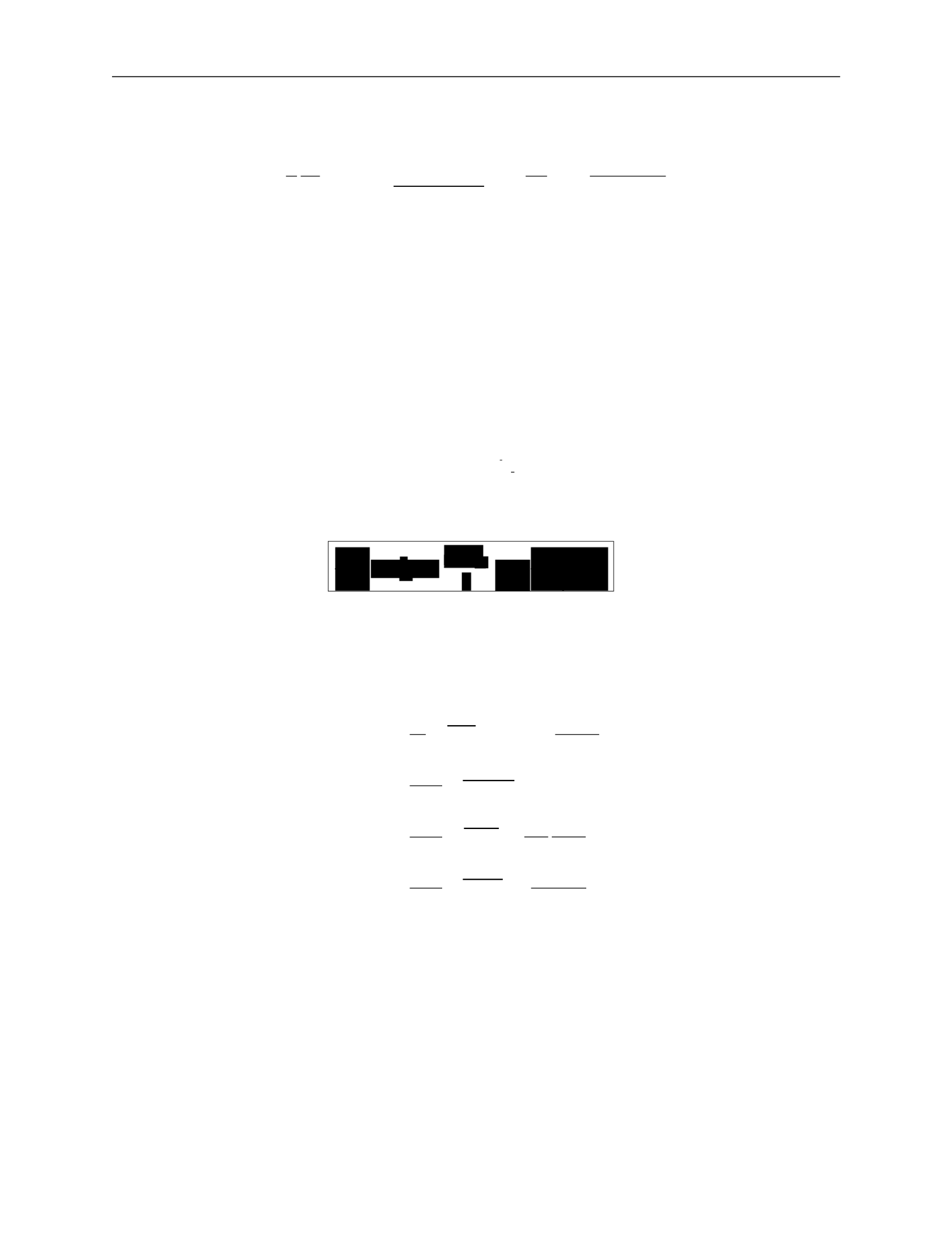
The simplified Jeans equation is:
1 ∂ 2(σ2
− σ ) ∂φ
GM (< r)
(nσ
2
) +
rr
t
=
−
=
−
(183)
where we’ve plugged in gravity as the force.
We have three limits we can look at:
•
σ
rr
•
σ
rr
•
σ
rr
σ
2
: nearly circular orbits
σ
2
: nearly radial orbits
= σ
2
: isotropic orbits
We define the anisotropy parameter:
σ
2
β
=
1
rr
(184)
which gives us a useful form of the Jeans equation for observations:
.
(185)
This depends only on radial components with uncertainty from
β
, assuming spherical sym-
metry and a steady-state system.
This can be simplified further to get mass estimates:
r2
1 ∂ 2 2βσ2
M (< r)
=
−
(nσ
)
+
2
=
−
rr
r
∂
(nσ
2
)
+
2β
G
2
=
rr
G
2
rr
r dn
+
n dr
rr
r
dσ
2
rr
+
2β
rr
(186)
2
=
rr
G
d ln n
+
d ln r
d ln σ2
rr
+
2β
d ln r
where the last line can be measured with observations.
Stability of stellar systems
The existence of equilibrium solutions to the collisionless Boltzmann equation does not assure
stability. Real stellar systems are subject to perturbations. What is important for stability?
1 ∂
2βσ2
σ
nσ
σ
n
∂r
r
2
r
∂r

3.
MODELLING GALAXIES
38
v
·
Luminosity-velocity relations:
We can relate properties of a galaxy to observables through several equations:
R
θ
=
(apparent size)
d
L
F
=
4πd
2
(158)
v
2
=
GM .
R
Introducing surface brightness Σ
F
L
d
2
Σ =
=
θ
2
4πd
2
R
2
(159)
L
v
4
then
=
4π
·
G2M 2
v
4
L =
Σ4πG
2
(M/L)
2
.
(160)
If we assume, for a given class of galaxies, that the surface brightness and the mass-to-light
ratio are the same, then
.
(161)
This introduces two important relations.
The Tully-Fischer relation is used for spiral galaxies and relates the maximum velocity in
the rotation curve
v
max
, which can be measured from HII spectra, and the luminosity:
4
max
.
(162)
The Faber-Jackson relation is used for ellipticals and relates the velocity dispersion
σ
v
to the
luminosity:
L
∝
σ
4
.
(163)
Thus, we can get an estimate of the intrinsic luminosity of a galaxy be measuring stel-
lar velocities. The constant of proportionality is roughly
L
∗
/(220 km/s)
4
, where
L
∗
is the
characteristic galaxy luminosity.
3.G
Phase-space distribution function
We have described the individual orbits in a potential, but this is not sufficient to describe
galactic dynamics. We want information of the configuration of all particles. Each star is
described by its position
→
x
and velocity
→
v
,
and we need to know this for all stars, i.e. how
stars are distributed in the 6D phase space
(
→
x
,
→
v
)
.
We define a phase-space distribution function
f
(
→
x
,
→
v
,
t)d3
→
x
d
3
→
v
(164)
∝
L
∝
v
3.
MODELLING GALAXIES
39
∈
dt
as the probability that at time
t
, a randomly chosen star has
(
→
x
∗
,
→
v
∗
)
([
→
x
,
→
x
+
d
→
x
]
,
[
→
v
,
→
v
+
d
→
v])
.
This
means
that
the function must be normalized for all
t
, i.e.
∫
f
(
→
x
,
→
v
,
t)d
3
→
x
d
3
→
v
= 1 .
(165)
Collisionless
Boltzmann
equation
:
We want to describe the time evolution of
f
(
→
x
,
→
v
,
t)
. Since probability cannot be destroyed,
the 6D continuity equation must hold.
We define the 6D phase-space vector
then
w
→
=
(
→
x
,
→
v
)
(166)
∂f
+
∂
f
w
→
˙
=
0 .
(167)
∂t
∂w
→
This is the same form as the standard 3D continuity equation. We can rewrite this by
expanding out
w
→
and using velocity
→
v
=
→
x
˙
and acceleration
→
a
=
→
v
˙
:
0
= ∂f +
∂
f
w
→
˙
∂t
∂w
→
∂f
∂
=
+
∂t
∂
→
x
(
f
→
x
˙
) +
∂
(
f
→
v
˙
)
∂
→
v
(168)
∂f
∂
∂
=
+
(
f
→
v
)
+
f
(
−
∇
→
φ)
∂t
∂
→
x
∂
→
v
∂f
∂f
∂φ
∂f
=
∂t
+
→
v
∂
→
x
−
∂
→
x
∂
→
v
.
This gives us the collisionless Boltzmann equation (CBE):
.
(169)
Note that another way to see this is by writing out
df
= 0
and taking the limits
lim
→x
→∞
= 0
and
lim
→v
→∞
= 0
.
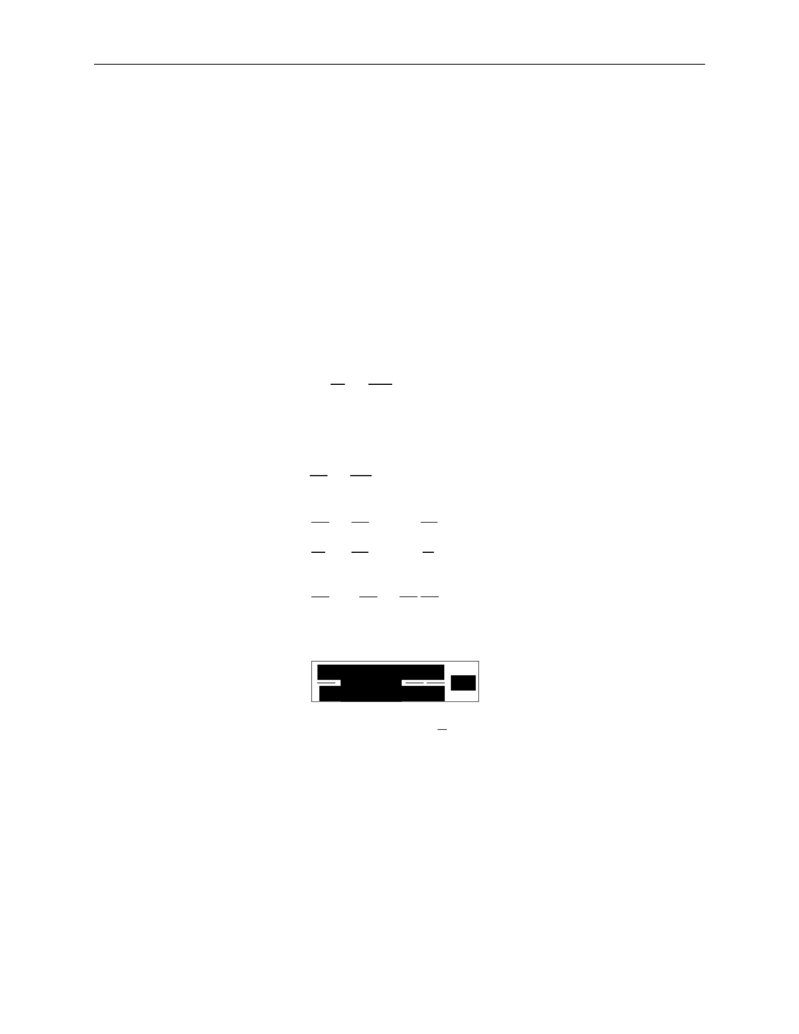
General Jeans equations:
A solution to the collisionless Boltzmann equation is difficult to obtain, so we instead study
moments of the CBE and the phase-space distribution.
Moments of the phase-space density give us some average quantities of the system.
a)
The first moment gives the density
n
of the system:
n
=
∫
f
d
3
→
v
.
(170)
∂t
−
3.
MODELLING GALAXIES
40
ij
∫
—
∫
∫
∫
±∞
—
i
n
i
i
j
n
i
j
∂
→
x
∂
→
v
∂
→
x
∂
→
v
∂
→
x
→v=
−∞
j
∂t
j
∂
→
x
j
∂
→
x
∂
→
v
2
b)
The second moment gives the average velocity
v
¯
i
:
v
¯
=
1
∫
v
f
d
3
→
v
.
(171)
c)
The third moment gives the velocity dispersion
σ
2
:
v v
=
1
∫
v v
f
d
3
→
v
ij
=
v
i
v
j
−
v
¯
i
v
¯
j
=
(v
i
−
v
¯
i
)(
v
j
−
v
¯
j
)
.
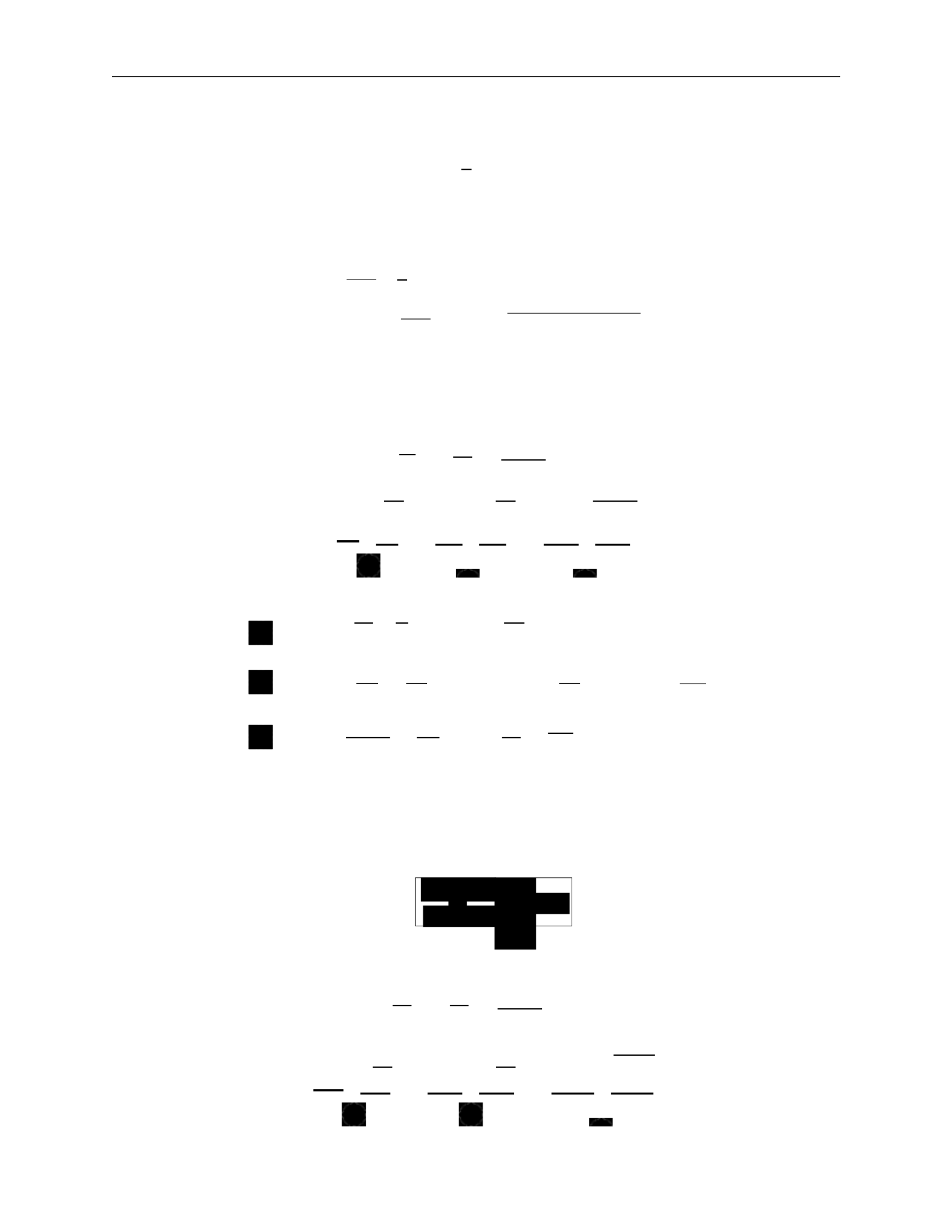
We now examine moments of the collisionless Boltzmann equation more closely. We break
each integral into three terms to simplify each individually.
i)
First moment:
d
3
→
v
∂f
∂t
∂f
+
→
v
∂
→
x
∂φ
∂f
=
0
∂
→
x
∂
→
v
∫
d
3
→
v
∂f +
∫
d
3
→
v
→
v
∂f
−
∫
d
3
→
v
∂φ
∂f =
0 (173)
∂t
` ˛
1
¸ x
∂
→
x
` ˛
2
¸ x
∂
→
x
∂
→
v
` ˛
3
¸ x
:
d
3
→
v
∂f =
∂
∂t ∂t
d
3
→
v
f
=
∂n
∂t
:
d
3
→
v
→
v
∂f
∂
→
x
∂
=
∂
→
x
d3
→
v
→
v
f
=
∂
∂
→
x
n
→
v
¯
=
Σ
∂
∂x
i
(
n
v
¯
i
)
(174)
:
∫
d
3
→
v
∂φ
∂f
=
∂φ
∫
d
3
→
v
∂f
=
∂φ [f ]
→v=+
∞
=
0
For the third term, we used the fact that phase-space distribution goes to 0 at
for
physical systems.
This gives us the 3D continuity equation:
j)
Second moment:
.
(175)
∫
d
3
→
v
vj
∂f
∂f
+
→
v
∂t
∂
→
x
∂φ
∂f
=
0
∂
→
x
∂
→
v
∫
d
3
→
v
v
∂f +
∫
d
3
→
v
v
→
v
∂f
−
∫
d
3
→
v
v
∂φ
∂f
=
0
(176)
` ˛
1
¸ x ` ˛
2
¸ x ` ˛
3
¸ x
1
2
3
∂n ∂
∂t
0
σ
∫
i
(172)

3.
MODELLING GALAXIES
41
ij
Σ
∫
i
∂x
∂x
j
∂t
∂t
j
∂t
j
∂t
∂t
∂x
i
∂t
∂t
j
∂x
i
using the continuity equation ∂n
=
−
Σ
∂
(
n
v
¯
)
j
∂
→
x
i
∂x
i
∂x
i
j
i
i
∂x
ij
i
j
∂x
j
∂v
j
v
i
=
−∞
i
∂v
∂t
∂x
i
∂x
ij
i
j
∂x
i
`
i
i
ij
i
∂x
i
∂v
:
∫
d
3
→
v
v
∂f =
∂
∫
d
3
→
v
v
f =
∂
(
n
v
¯
) =
∂
n
v
¯
+
n
∂
v
¯
j
=
−
v
¯
Σ
∂
(
n
v
¯
) +
n
∂
v
¯
j
=
n
∂
v
¯
j
−
v
¯
Σ
∂
(
n
v
¯
)
∂t
∂x
i
i
to go from the first line to the second
:
∫
d
3
→
v
v
→
v
∂f
=
∫
d
3
→
v
v
Σ
v
∂f =
Σ
∂
∫
d
3
→
v
v v
f
= nv
j
v
i
`
= n
˛ ¸
σ
2
+
x
v
¯
i
v
¯
j
=
Σ
∂
n
σ
2
+
v
¯
v
¯
:
∫
d
3
→
v
v
∂φ
∂f
=
∫
d
3
→
v
v
Σ
∂φ
∂f
=
Σ
∂φ
∫
d
3
→
v
v
∂f
(177)
((k, l, i) are permutations of (1, 2, 3))
=
∂φ
dv
∂x
k
∫
dv
l
∫
dv
i
∂f
v
j
∂v
=
[v
f
]
˛
v
¸
i
=+
∞
−
x
∫
dv ∂v
j
f
= 0
−
∫
dv
i
δ
ij
f
=
−
Σ
∂φ
∫
dv
∫
dv
l
∫
dv
i
δ
ij
f
i
i
=
−
Σ
∂φ
∫
d
3
→
v
δ
f
i
i
∂φ
=
−
n∂x
j
Plugging each term back in, we get
n
∂
v
¯
j
−
v
¯
Σ
∂
(
n
v
¯
) +
Σ
∂
n
σ
2
+
v
¯
v
¯
+
n
∂φ
=
0
(178)
i
i
i
i
i
i
i
i
i
i
i
1
2
3
j
j
i
j
i
i
j
∂
→
x
∂
→
v
j
i
i
i
j
k

3.
MODELLING GALAXIES
42
Σ
v
¯
2
2
∂t
j
∂x
i
∂x
ij
i
∂x
i
i
j
∂x
j
=
(
n
v
¯
i
)
∂
x
v
¯
j
+
v
¯
j
∂x
(
n
v
¯
i
)
∂t
i
∂x
j
∂x
ij
∂x
—
1
Σ
∂(nσ
ij
) :
pressure
∂t
i
i
i
i
i
i
i
i
j
which we can rewrite
n
∂
v
¯
j
−
v
¯
Σ
∂
(
n
v
¯
)
+
Σ
∂
(nσ
2
)+
Σ
∂
(
n
v
¯
v
¯
)
+n
∂φ
=
0
`
Σ˛¸
∂
x
Σ
∂
(179)
where the two underlined terms cancel. This gives us
n
∂
v
¯
j
+
Σ
(
n
v
¯
)
∂
v
¯
+
Σ
∂
(nσ
2
) +
n
∂φ
=
0 .
(180)
This is the Jeans equation, often written
(181)
Each term can be physically interpreted:
∂
v
¯
j
∂t
∂
v
¯
j
i
∂x
: acceleration of fluid
: kinematic viscosity/shear
i
i
2
(182)
n
∂x
i
∂φ
−
∂x
j
: gravity
Jeans
equations
in
spherical
systems
:
We can convert to spherical coordinates and take velocity moments to give us the Jeans
equations in spherical coordinates. This is complicated!
To simplify, we take the radial Jeans equation and focus on steady-state symmetric systems.
Implications:
∂
=
0
since we have steady state
•
v
¯
r
=
0
otherwise we have net radial motion
•
v
¯
θ
=
v
¯
φ
=
0
or the symmetry is broken
•
σ
rφ
=
0
or the symmetry is broken
2
•
σ
φφ
≡
σ
or the symmetry is broken.
2
2
rθ
θθ
t
∂φ
1
∂t
•
=
σ
=
σ
i
i
i
i
i
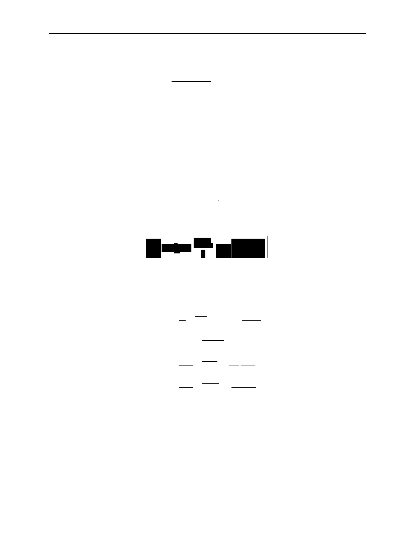
3.
MODELLING GALAXIES
43
2
2
2
2
t
t
t
— t
2
rr
rσ
rσ
rσ
rr
r
∂r
G
n
∂r
rr
—
dr
2
—
The simplified Jeans equation is:
1 ∂ 2(σ2
− σ ) ∂φ
GM (< r)
(nσ
2
) +
rr
t
=
−
=
−
(183)
where we’ve plugged in gravity as the force.
We have three limits we can look at:
•
σ
rr
•
σ
rr
•
σ
rr
σ
2
: nearly circular orbits
σ
2
: nearly radial orbits
= σ
2
: isotropic orbits
We define the anisotropy parameter:
σ
2
β
=
1
rr
(184)
which gives us a useful form of the Jeans equation for observations:
.
(185)
This depends only on radial components with uncertainty from
β
, assuming spherical sym-
metry and a steady-state system.
This can be simplified further to get mass estimates:
r2
1 ∂ 2 2βσ2
M (< r)
=
−
(nσ
)
+
2
=
−
rr
r
∂
(nσ
2
)
+
2β
G
2
=
rr
G
2
rr
r dn
+
n dr
rr
r
dσ
2
rr
+
2β
rr
(186)
2
=
rr
G
d ln n
+
d ln r
d ln σ2
rr
+
2β
d ln r
where the last line can be measured with observations.
Stability of stellar systems
The existence of equilibrium solutions to the collisionless Boltzmann equation does not assure stability.
Real stellar systems are subject to perturbations. What is important for stability?
1 ∂
2βσ2
σ
nσ
σ
n
∂r
r
2
r
∂r
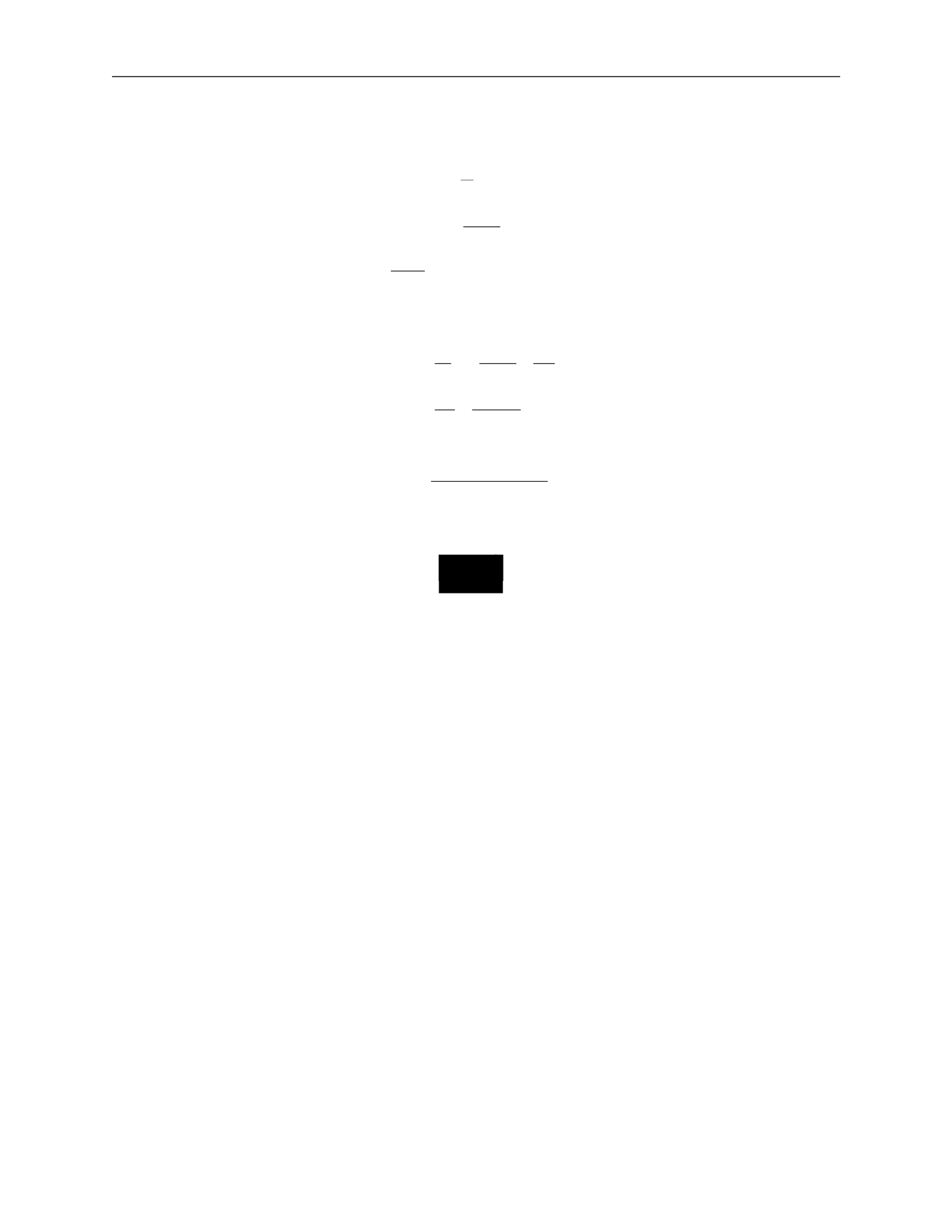
3.
MODELLING GALAXIES
38
v
·
Luminosity-velocity relations:
We can relate properties of a galaxy to observables through several equations:
R
θ
=
(apparent size)
d
L
F
=
4πd
2
(158)
v
2
=
GM .
R
Introducing surface brightness Σ
F
L
d
2
Σ =
=
θ
2
4πd
2
R
2
(159)
L
v
4
then
=
4π
·
G2M 2
v
4
L =
Σ4πG
2
(M/L)
2
.
(160)
If we assume, for a given class of galaxies, that the surface brightness and the mass-to-light
ratio are the same, then
.
(161)
This introduces two important relations.
The Tully-Fischer relation is used for spiral galaxies and relates the maximum velocity in
the rotation curve
v
max
, which can be measured from HII spectra, and the luminosity:
4
max
.
(162)
The Faber-Jackson relation is used for ellipticals and relates the velocity dispersion
σ
v
to the
luminosity:
L
∝
σ
4
.
(163)
Thus, we can get an estimate of the intrinsic luminosity of a galaxy be measuring stel-
lar velocities. The constant of proportionality is roughly
L
∗
/(220 km/s)
4
, where
L
∗
is the
characteristic galaxy luminosity.
3.H
Phase-space distribution function
We have described the individual orbits in a potential, but this is not sufficient to describe
galactic dynamics. We want information of the configuration of all particles. Each star is
described by its position
→
x
and velocity
→
v
,
and we need to know this for all stars, i.e. how
stars are distributed in the 6D phase space
(
→
x
,
→
v
)
.
We define a phase-space distribution function
f
(
→
x
,
→
v
,
t)d3
→
x
d
3
→
v
(164)
∝
L
∝
v
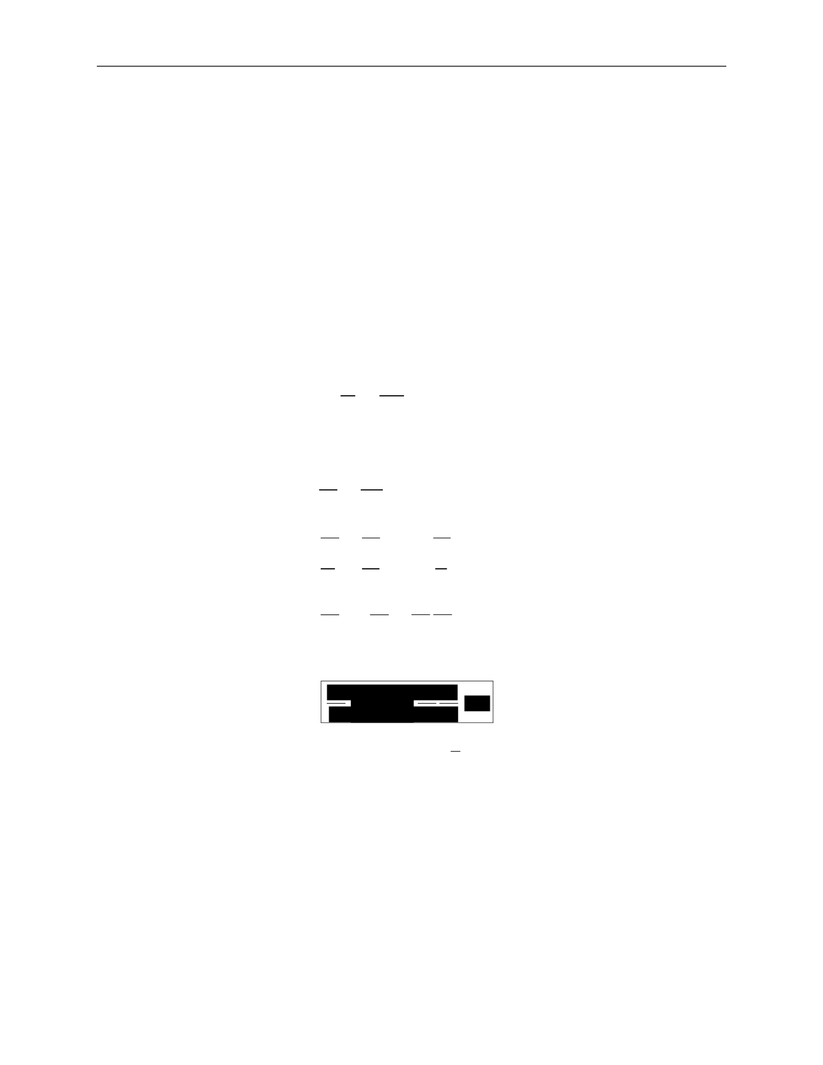
3.
MODELLING GALAXIES
39
∈
dt
as the probability that at time
t
, a randomly chosen star has
(
→
x
∗
,
→
v
∗
)
([
→
x
,
→
x
+
d
→
x
]
,
[
→
v
,
→
v
+
d
→
v])
.
This
means
that
the function must be normalized for all
t
, i.e.
∫
f
(
→
x
,
→
v
,
t)d
3
→
x
d
3
→
v
= 1 .
(165)
Collisionless
Boltzmann
equation
:
We want to describe the time evolution of
f
(
→
x
,
→
v
,
t)
. Since probability cannot be destroyed,
the 6D continuity equation must hold.
We define the 6D phase-space vector
then
w
→
=
(
→
x
,
→
v
)
(166)
∂f
+
∂
f
w
→
˙
=
0 .
(167)
∂t
∂w
→
This is the same form as the standard 3D continuity equation. We can rewrite this by
expanding out
w
→
and using velocity
→
v
=
→
x
˙
and acceleration
→
a
=
→
v
˙
:
0
= ∂f +
∂
f
w
→
˙
∂t
∂w
→
∂f
∂
=
+
∂t
∂
→
x
(
f
→
x
˙
) +
∂
(
f
→
v
˙
)
∂
→
v
(168)
∂f
∂
∂
=
+
(
f
→
v
)
+
f
(
−
∇
→
φ)
∂t
∂
→
x
∂
→
v
∂f
∂f
∂φ
∂f
=
∂t
+
→
v
∂
→
x
−
∂
→
x
∂
→
v
.
This gives us the collisionless Boltzmann equation (CBE):
.
(169)
Note that another way to see this is by writing out
df
= 0
and taking the limits
lim
→x
→∞
= 0
and
lim
→v
→∞
= 0
.
General Jeans equations:
A solution to the collisionless Boltzmann equation is difficult to obtain, so we instead study
moments of the CBE and the phase-space distribution.
Moments of the phase-space density give us some average quantities of the system.
a)
The first moment gives the density
n
of the system:
n
=
∫
f
d
3
→
v
.
(170)
∂t
−

3.
MODELLING GALAXIES
40
ij
∫
—
∫
∫
∫
±∞
—
i
n
i
i
j
n
i
j
∂
→
x
∂
→
v
∂
→
x
∂
→
v
∂
→
x
→v=
−∞
j
∂t
j
∂
→
x
j
∂
→
x
∂
→
v
2
b)
The second moment gives the average velocity
v
¯
i
:
v
¯
=
1
∫
v
f
d
3
→
v
.
(171)
c)
The third moment gives the velocity dispersion
σ
2
:
v v
=
1
∫
v v
f
d
3
→
v
ij
=
v
i
v
j
−
v
¯
i
v
¯
j
=
(v
i
−
v
¯
i
)(
v
j
−
v
¯
j
)
.
We now examine moments of the collisionless Boltzmann equation more closely. We break
each integral into three terms to simplify each individually.
k)
First moment:
d
3
→
v
∂f
∂t
∂f
+
→
v
∂
→
x
∂φ
∂f
=
0
∂
→
x
∂
→
v
∫
d
3
→
v
∂f +
∫
d
3
→
v
→
v
∂f
−
∫
d
3
→
v
∂φ
∂f =
0 (173)
∂t
` ˛
1
¸ x
∂
→
x
` ˛
2
¸ x
∂
→
x
∂
→
v
` ˛
3
¸ x
:
d
3
→
v
∂f =
∂
∂t ∂t
d
3
→
v
f
=
∂n
∂t
:
d
3
→
v
→
v
∂f
∂
→
x
∂
=
∂
→
x
d3
→
v
→
v
f
=
∂
∂
→
x
n
→
v
¯
=
Σ
∂
∂x
i
(
n
v
¯
i
)
(174)
:
∫
d
3
→
v
∂φ
∂f
=
∂φ
∫
d
3
→
v
∂f
=
∂φ [f ]
→v=+
∞
=
0
For the third term, we used the fact that phase-space distribution goes to 0 at
for
physical systems.
This gives us the 3D continuity equation:
l)
Second moment:
.
(175)
∫
d
3
→
v
vj
∂f
∂f
+
→
v
∂t
∂
→
x
∂φ
∂f
=
0
∂
→
x
∂
→
v
∫
d
3
→
v
v
∂f +
∫
d
3
→
v
v
→
v
∂f
−
∫
d
3
→
v
v
∂φ
∂f
=
0
(176)
` ˛
1
¸ x ` ˛
2
¸ x ` ˛
3
¸ x
1
2
3
∂n ∂
∂t
0
σ
∫
i
(172)

3.
MODELLING GALAXIES
41
ij
Σ
∫
i
∂x
∂x
j
∂t
∂t
j
∂t
j
∂t
∂t
∂x
i
∂t
∂t
j
∂x
i
using the continuity equation ∂n
=
−
Σ
∂
(
n
v
¯
)
j
∂
→
x
i
∂x
i
∂x
i
j
i
i
∂x
ij
i
j
∂x
j
∂v
j
v
i
=
−∞
i
∂v
∂t
∂x
i
∂x
ij
i
j
∂x
i
`
i
i
ij
i
∂x
i
∂v
:
∫
d
3
→
v
v
∂f =
∂
∫
d
3
→
v
v
f =
∂
(
n
v
¯
) =
∂
n
v
¯
+
n
∂
v
¯
j
=
−
v
¯
Σ
∂
(
n
v
¯
) +
n
∂
v
¯
j
=
n
∂
v
¯
j
−
v
¯
Σ
∂
(
n
v
¯
)
∂t
∂x
i
i
to go from the first line to the second
:
∫
d
3
→
v
v
→
v
∂f
=
∫
d
3
→
v
v
Σ
v
∂f =
Σ
∂
∫
d
3
→
v
v v
f
= nv
j
v
i
`
= n
˛ ¸
σ
2
+
x
v
¯
i
v
¯
j
=
Σ
∂
n
σ
2
+
v
¯
v
¯
:
∫
d
3
→
v
v
∂φ
∂f
=
∫
d
3
→
v
v
Σ
∂φ
∂f
=
Σ
∂φ
∫
d
3
→
v
v
∂f
(177)
((k, l, i) are permutations of (1, 2, 3))
=
∂φ
dv
∂x
k
∫
dv
l
∫
dv
i
∂f
v
j
∂v
=
[v
f
]
˛
v
¸
i
=+
∞
−
x
∫
dv ∂v
j
f
= 0
−
∫
dv
i
δ
ij
f
=
−
Σ
∂φ
∫
dv
∫
dv
l
∫
dv
i
δ
ij
f
i
i
=
−
Σ
∂φ
∫
d
3
→
v
δ
f
i
i
∂φ
=
−
n∂x
j
Plugging each term back in, we get
n
∂
v
¯
j
−
v
¯
Σ
∂
(
n
v
¯
) +
Σ
∂
n
σ
2
+
v
¯
v
¯
+
n
∂φ
=
0
(178)
i
i
i
i
i
i
i
i
i
i
i
1
2
3
j
j
i
j
i
i
j
∂
→
x
∂
→
v
j
i
i
i
j
k

3.
MODELLING GALAXIES
42
Σ
v
¯
2
2
∂t
j
∂x
i
∂x
ij
i
∂x
i
i
j
∂x
j
=
(
n
v
¯
i
)
∂
x
v
¯
j
+
v
¯
j
∂x
(
n
v
¯
i
)
∂t
i
∂x
j
∂x
ij
∂x
—
1
Σ
∂(nσ
ij
) :
pressure
∂t
i
i
i
i
i
i
i
i
j
which we can rewrite
n
∂
v
¯
j
−
v
¯
Σ
∂
(
n
v
¯
)
+
Σ
∂
(nσ
2
)+
Σ
∂
(
n
v
¯
v
¯
)
+n
∂φ
=
0
`
Σ˛¸
∂
x
Σ
∂
(179)
where the two underlined terms cancel. This gives us
n
∂
v
¯
j
+
Σ
(
n
v
¯
)
∂
v
¯
+
Σ
∂
(nσ
2
) +
n
∂φ
=
0 .
(180)
This is the Jeans equation, often written
(181)
Each term can be physically interpreted:
∂
v
¯
j
∂t
∂
v
¯
j
i
∂x
: acceleration of fluid
: kinematic viscosity/shear
i
i
2
(182)
n
∂x
i
∂φ
−
∂x
j
: gravity
Jeans
equations
in
spherical
systems
:
We can convert to spherical coordinates and take velocity moments to give us the Jeans
equations in spherical coordinates. This is complicated!
To simplify, we take the radial Jeans equation and focus on steady-state symmetric systems.
Implications:
∂
=
0
since we have steady state
•
v
¯
r
=
0
otherwise we have net radial motion
•
v
¯
θ
=
v
¯
φ
=
0
or the symmetry is broken
•
σ
rφ
=
0
or the symmetry is broken
2
•
σ
φφ
≡
σ
or the symmetry is broken.
2
2
rθ
θθ
t
∂φ
1
∂t
•
=
σ
=
σ
i
i
i
i
i
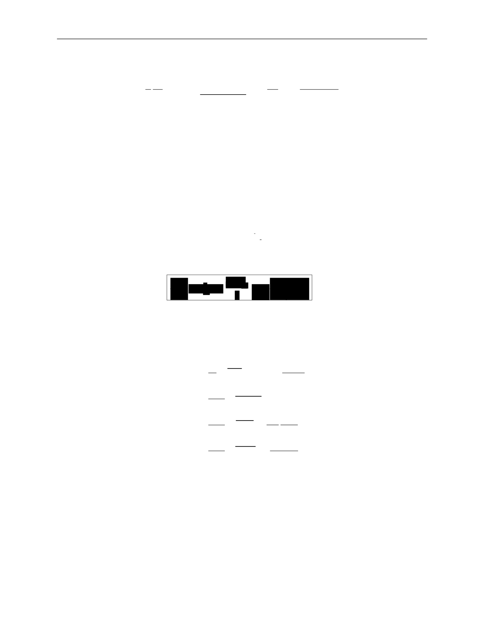
3.
MODELLING GALAXIES
43
2
2
2
2
t
t
t
— t
2
rr
rσ
rσ
rσ
rr
r
∂r
G
n
∂r
rr
—
dr
2
—
The simplified Jeans equation is:
1 ∂ 2(σ2
− σ ) ∂φ
GM (< r)
(nσ
2
) +
rr
t
=
−
=
−
(183)
where we’ve plugged in gravity as the force.
We have three limits we can look at:
•
σ
rr
•
σ
rr
•
σ
rr
σ
2
: nearly circular orbits
σ
2
: nearly radial orbits
= σ
2
: isotropic orbits
We define the anisotropy parameter:
σ
2
β
=
1
rr
(184)
which gives us a useful form of the Jeans equation for observations:
.
(185)
This depends only on radial components with uncertainty from
β
, assuming spherical sym-
metry and a steady-state system.
This can be simplified further to get mass estimates:
r2
1 ∂ 2 2βσ2
M (< r)
=
−
(nσ
)
+
2
=
−
rr
r
∂
(nσ
2
)
+
2β
G
2
=
rr
G
2
rr
r dn
+
n dr
rr
r
dσ
2
rr
+
2β
rr
(186)
2
=
rr
G
d ln n
+
d ln r
d ln σ2
rr
+
2β
d ln r
where the last line can be measured with observations.
Stability of stellar systems
The existence of equilibrium solutions to the collisionless Boltzmann equation does not assure
stability. Real stellar systems are subject to perturbations. What is important for stability?
1 ∂
2βσ2
σ
nσ
σ
n
∂r
r
2
r
∂r
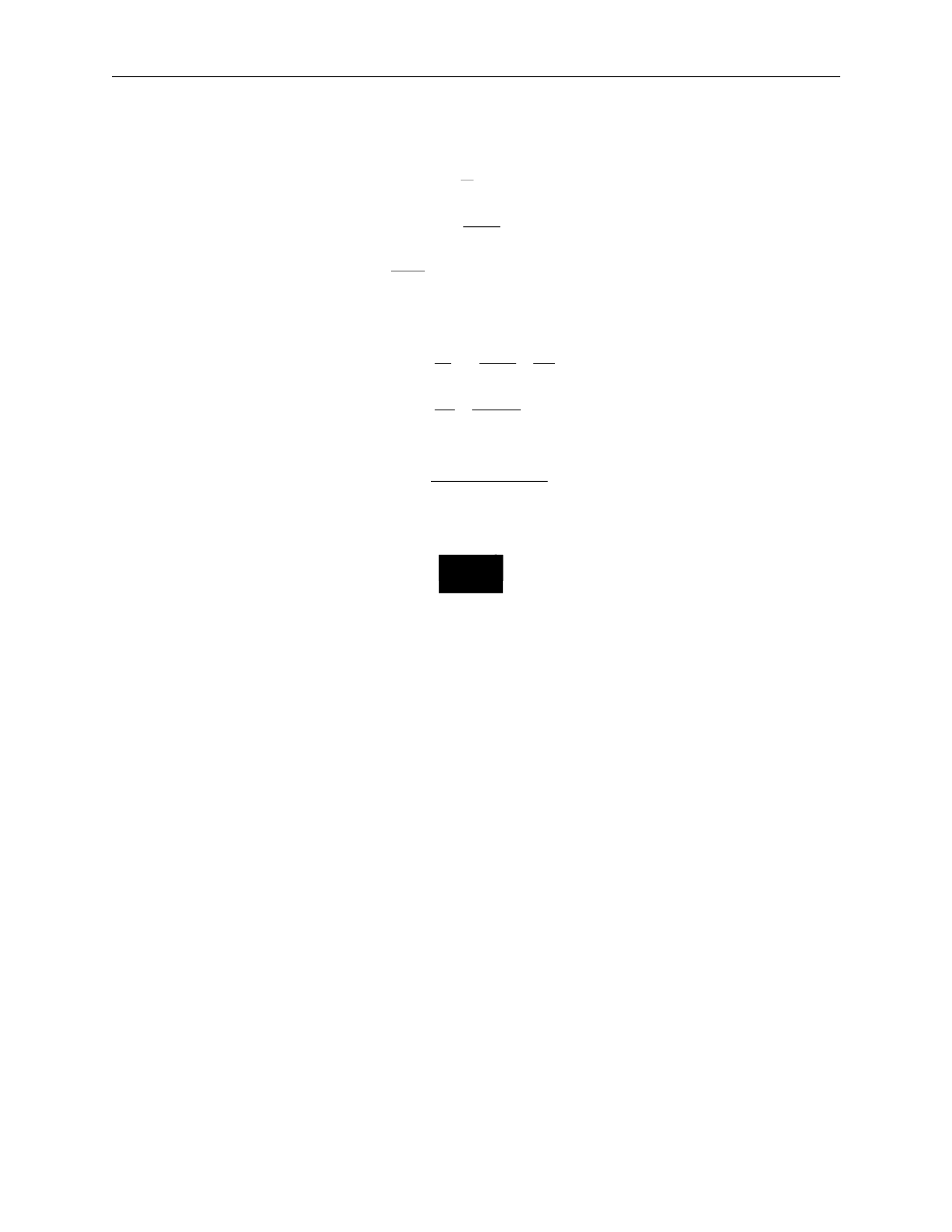
3.
MODELLING GALAXIES
38
v
·
Luminosity-velocity relations:
We can relate properties of a galaxy to observables through several equations:
R
θ
=
(apparent size)
d
L
F
=
4πd
2
(158)
v
2
=
GM .
R
Introducing surface brightness Σ
F
L
d
2
Σ =
=
θ
2
4πd
2
R
2
(159)
L
v
4
then
=
4π
·
G2M 2
v
4
L =
Σ4πG
2
(M/L)
2
.
(160)
If we assume, for a given class of galaxies, that the surface brightness and the mass-to-light
ratio are the same, then
.
(161)
This introduces two important relations.
The Tully-Fischer relation is used for spiral galaxies and relates the maximum velocity in
the rotation curve
v
max
, which can be measured from HII spectra, and the luminosity:
4
max
.
(162)
The Faber-Jackson relation is used for ellipticals and relates the velocity dispersion
σ
v
to the
luminosity:
L
∝
σ
4
.
(163)
Thus, we can get an estimate of the intrinsic luminosity of a galaxy be measuring stel-
lar velocities. The constant of proportionality is roughly
L
∗
/(220 km/s)
4
, where
L
∗
is the
characteristic galaxy luminosity.
3.I
Phase-space distribution function
We have described the individual orbits in a potential, but this is not sufficient to describe
galactic dynamics. We want information of the configuration of all particles. Each star is
described by its position
→
x
and velocity
→
v
,
and we need to know this for all stars, i.e. how
stars are distributed in the 6D phase space
(
→
x
,
→
v
)
.
We define a phase-space distribution function
f
(
→
x
,
→
v
,
t)d3
→
x
d
3
→
v
(164)
∝
L
∝
v
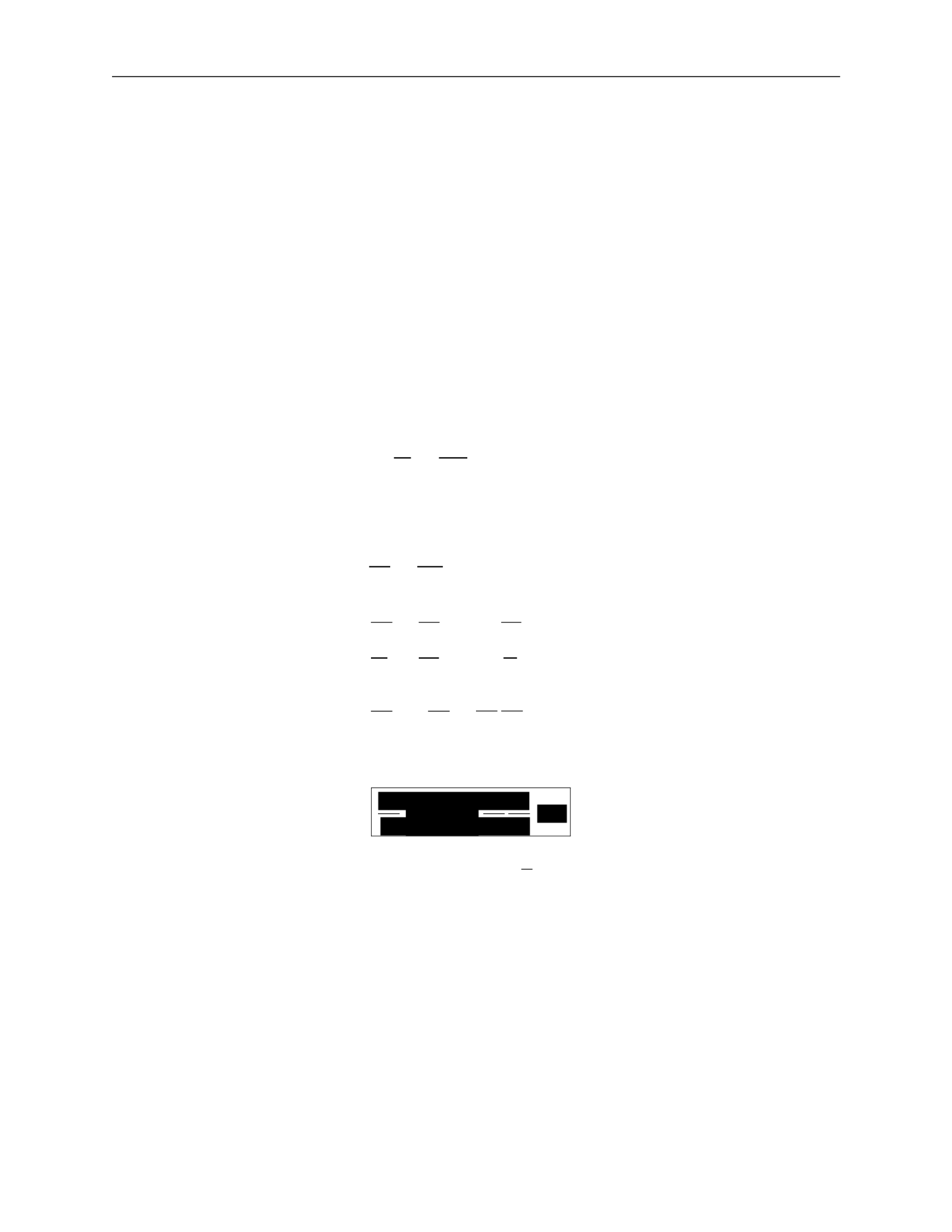
3.
MODELLING GALAXIES
39
∈
dt
as the probability that at time
t
, a randomly chosen star has
(
→
x
∗
,
→
v
∗
)
([
→
x
,
→
x
+
d
→
x
]
,
[
→
v
,
→
v
+
d
→
v])
.
This
means
that
the function must be normalized for all
t
, i.e.
∫
f
(
→
x
,
→
v
,
t)d
3
→
x
d
3
→
v
= 1 .
(165)
Collisionless
Boltzmann
equation
:
We want to describe the time evolution of
f
(
→
x
,
→
v
,
t)
. Since probability cannot be destroyed,
the 6D continuity equation must hold.
We define the 6D phase-space vector
then
w
→
=
(
→
x
,
→
v
)
(166)
∂f
+
∂
f
w
→
˙
=
0 .
(167)
∂t
∂w
→
This is the same form as the standard 3D continuity equation. We can rewrite this by
expanding out
w
→
and using velocity
→
v
=
→
x
˙
and acceleration
→
a
=
→
v
˙
:
0
= ∂f +
∂
f
w
→
˙
∂t
∂w
→
∂f
∂
=
+
∂t
∂
→
x
(
f
→
x
˙
) +
∂
(
f
→
v
˙
)
∂
→
v
(168)
∂f
∂
∂
=
+
(
f
→
v
)
+
f
(
−
∇
→
φ)
∂t
∂
→
x
∂
→
v
∂f
∂f
∂φ
∂f
=
∂t
+
→
v
∂
→
x
−
∂
→
x
∂
→
v
.
This gives us the collisionless Boltzmann equation (CBE):
.
(169)
Note that another way to see this is by writing out
df
= 0
and taking the limits
lim
→x
→∞
= 0
and
lim
→v
→∞
= 0
.
General Jeans equations:
A solution to the collisionless Boltzmann equation is difficult to obtain, so we instead study
moments of the CBE and the phase-space distribution.
Moments of the phase-space density give us some average quantities of the system.
a)
The first moment gives the density
n
of the system:
n
=
∫
f
d
3
→
v
.
(170)
∂t
−
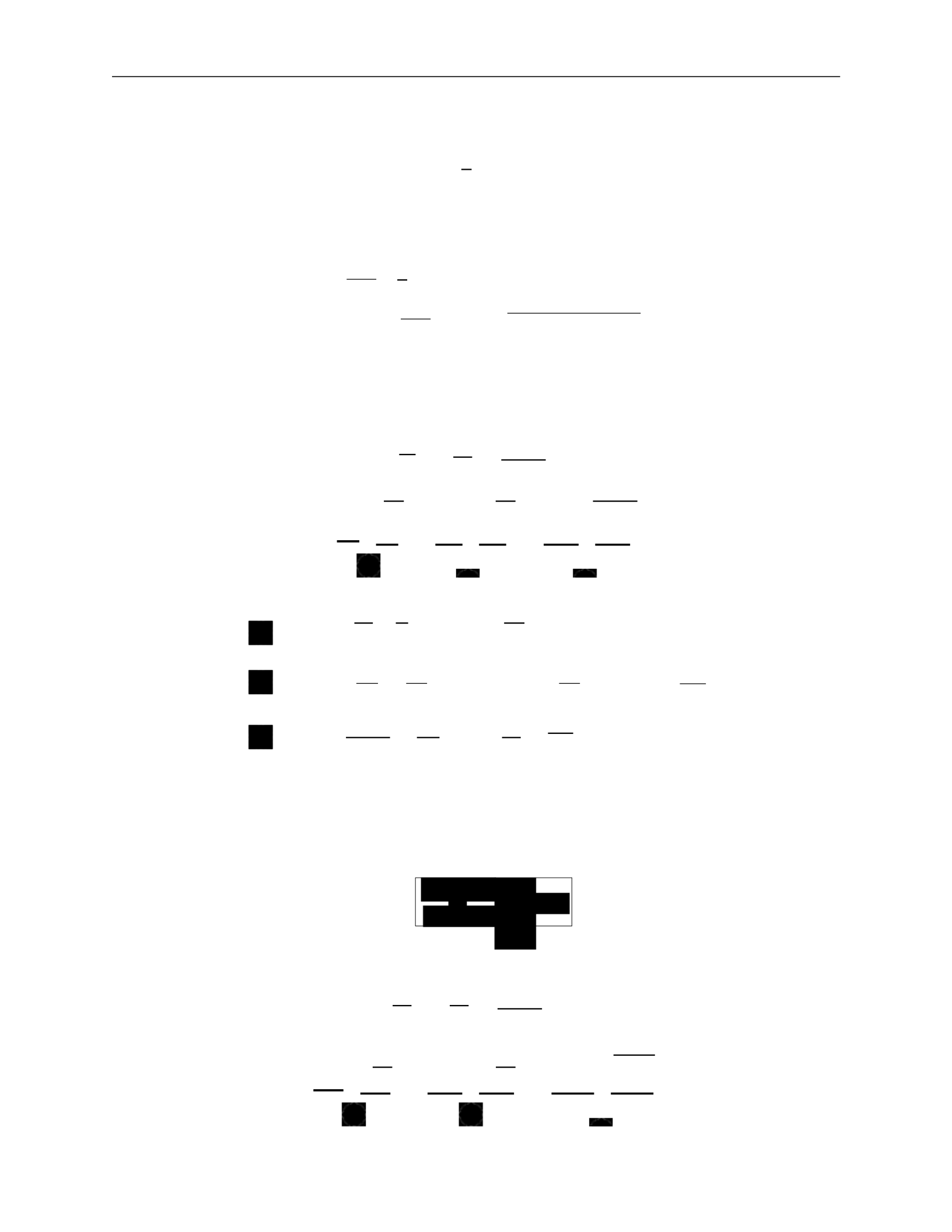
3.
MODELLING GALAXIES
40
ij
∫
—
∫
∫
∫
±∞
—
i
n
i
i
j
n
i
j
∂
→
x
∂
→
v
∂
→
x
∂
→
v
∂
→
x
→v=
−∞
j
∂t
j
∂
→
x
j
∂
→
x
∂
→
v
2
b)
The second moment gives the average velocity
v
¯
i
:
v
¯
=
1
∫
v
f
d
3
→
v
.
(171)
c)
The third moment gives the velocity dispersion
σ
2
:
v v
=
1
∫
v v
f
d
3
→
v
ij
=
v
i
v
j
−
v
¯
i
v
¯
j
=
(v
i
−
v
¯
i
)(
v
j
−
v
¯
j
)
.
We now examine moments of the collisionless Boltzmann equation more closely. We break
each integral into three terms to simplify each individually.
m)
First moment:
d
3
→
v
∂f
∂t
∂f
+
→
v
∂
→
x
∂φ
∂f
=
0
∂
→
x
∂
→
v
∫
d
3
→
v
∂f +
∫
d
3
→
v
→
v
∂f
−
∫
d
3
→
v
∂φ
∂f =
0 (173)
∂t
` ˛
1
¸ x
∂
→
x
` ˛
2
¸ x
∂
→
x
∂
→
v
` ˛
3
¸ x
:
d
3
→
v
∂f =
∂
∂t ∂t
d
3
→
v
f
=
∂n
∂t
:
d
3
→
v
→
v
∂f
∂
→
x
∂
=
∂
→
x
d3
→
v
→
v
f
=
∂
∂
→
x
n
→
v
¯
=
Σ
∂
∂x
i
(
n
v
¯
i
)
(174)
:
∫
d
3
→
v
∂φ
∂f
=
∂φ
∫
d
3
→
v
∂f
=
∂φ [f ]
→v=+
∞
=
0
For the third term, we used the fact that phase-space distribution goes to 0 at
for
physical systems.
This gives us the 3D continuity equation:
n)
Second moment:
.
(175)
∫
d
3
→
v
vj
∂f
∂f
+
→
v
∂t
∂
→
x
∂φ
∂f
=
0
∂
→
x
∂
→
v
∫
d
3
→
v
v
∂f +
∫
d
3
→
v
v
→
v
∂f
−
∫
d
3
→
v
v
∂φ
∂f
=
0
(176)
` ˛
1
¸ x ` ˛
2
¸ x ` ˛
3
¸ x
1
2
3
∂n ∂
∂t
0
σ
∫
i
(172)

3.
MODELLING GALAXIES
41
ij
Σ
∫
i
∂x
∂x
j
∂t
∂t
j
∂t
j
∂t
∂t
∂x
i
∂t
∂t
j
∂x
i
using the continuity equation ∂n
=
−
Σ
∂
(
n
v
¯
)
j
∂
→
x
i
∂x
i
∂x
i
j
i
i
∂x
ij
i
j
∂x
j
∂v
j
v
i
=
−∞
i
∂v
∂t
∂x
i
∂x
ij
i
j
∂x
i
`
i
i
ij
i
∂x
i
∂v
:
∫
d
3
→
v
v
∂f =
∂
∫
d
3
→
v
v
f =
∂
(
n
v
¯
) =
∂
n
v
¯
+
n
∂
v
¯
j
=
−
v
¯
Σ
∂
(
n
v
¯
) +
n
∂
v
¯
j
=
n
∂
v
¯
j
−
v
¯
Σ
∂
(
n
v
¯
)
∂t
∂x
i
i
to go from the first line to the second
:
∫
d
3
→
v
v
→
v
∂f
=
∫
d
3
→
v
v
Σ
v
∂f =
Σ
∂
∫
d
3
→
v
v v
f
= nv
j
v
i
`
= n
˛ ¸
σ
2
+
x
v
¯
i
v
¯
j
=
Σ
∂
n
σ
2
+
v
¯
v
¯
:
∫
d
3
→
v
v
∂φ
∂f
=
∫
d
3
→
v
v
Σ
∂φ
∂f
=
Σ
∂φ
∫
d
3
→
v
v
∂f
(177)
((k, l, i) are permutations of (1, 2, 3))
=
∂φ
dv
∂x
k
∫
dv
l
∫
dv
i
∂f
v
j
∂v
=
[v
f
]
˛
v
¸
i
=+
∞
−
x
∫
dv ∂v
j
f
= 0
−
∫
dv
i
δ
ij
f
=
−
Σ
∂φ
∫
dv
∫
dv
l
∫
dv
i
δ
ij
f
i
i
=
−
Σ
∂φ
∫
d
3
→
v
δ
f
i
i
∂φ
=
−
n∂x
j
Plugging each term back in, we get
n
∂
v
¯
j
−
v
¯
Σ
∂
(
n
v
¯
) +
Σ
∂
n
σ
2
+
v
¯
v
¯
+
n
∂φ
=
0
(178)
i
i
i
i
i
i
i
i
i
i
i
1
2
3
j
j
i
j
i
i
j
∂
→
x
∂
→
v
j
i
i
i
j
k

3.
MODELLING GALAXIES
42
Σ
v
¯
2
2
∂t
j
∂x
i
∂x
ij
i
∂x
i
i
j
∂x
j
=
(
n
v
¯
i
)
∂
x
v
¯
j
+
v
¯
j
∂x
(
n
v
¯
i
)
∂t
i
∂x
j
∂x
ij
∂x
—
1
Σ
∂(nσ
ij
) :
pressure
∂t
i
i
i
i
i
i
i
i
j
which we can rewrite
n
∂
v
¯
j
−
v
¯
Σ
∂
(
n
v
¯
)
+
Σ
∂
(nσ
2
)+
Σ
∂
(
n
v
¯
v
¯
)
+n
∂φ
=
0
`
Σ˛¸
∂
x
Σ
∂
(179)
where the two underlined terms cancel. This gives us
n
∂
v
¯
j
+
Σ
(
n
v
¯
)
∂
v
¯
+
Σ
∂
(nσ
2
) +
n
∂φ
=
0 .
(180)
This is the Jeans equation, often written
(181)
Each term can be physically interpreted:
∂
v
¯
j
∂t
∂
v
¯
j
i
∂x
: acceleration of fluid
: kinematic viscosity/shear
i
i
2
(182)
n
∂x
i
∂φ
−
∂x
j
: gravity
Jeans
equations
in
spherical
systems
:
We can convert to spherical coordinates and take velocity moments to give us the Jeans
equations in spherical coordinates. This is complicated!
To simplify, we take the radial Jeans equation and focus on steady-state symmetric systems.
Implications:
∂
=
0
since we have steady state
•
v
¯
r
=
0
otherwise we have net radial motion
•
v
¯
θ
=
v
¯
φ
=
0
or the symmetry is broken
•
σ
rφ
=
0
or the symmetry is broken
2
•
σ
φφ
≡
σ
or the symmetry is broken.
2
2
rθ
θθ
t
∂φ
1
∂t
•
=
σ
=
σ
i
i
i
i
i

3.
MODELLING GALAXIES
43
2
2
2
2
t
t
t
— t
2
rr
rσ
rσ
rσ
rr
r
∂r
G
n
∂r
rr
—
dr
2
—
The simplified Jeans equation is:
1 ∂ 2(σ2
− σ ) ∂φ
GM (< r)
(nσ
2
) +
rr
t
=
−
=
−
(183)
where we’ve plugged in gravity as the force.
We have three limits we can look at:
•
σ
rr
•
σ
rr
•
σ
rr
σ
2
: nearly circular orbits
σ
2
: nearly radial orbits
= σ
2
: isotropic orbits
We define the anisotropy parameter:
σ
2
β
=
1
rr
(184)
which gives us a useful form of the Jeans equation for observations:
.
(185)
This depends only on radial components with uncertainty from
β
, assuming spherical sym-
metry and a steady-state system.
This can be simplified further to get mass estimates:
r2
1 ∂ 2 2βσ2
M (< r)
=
−
(nσ
)
+
2
=
−
rr
r
∂
(nσ
2
)
+
2β
G
2
=
rr
G
2
rr
r dn
+
n dr
rr
r
dσ
2
rr
+
2β
rr
(186)
2
=
rr
G
d ln n
+
d ln r
d ln σ2
rr
+
2β
d ln r
where the last line can be measured with observations.
Stability of stellar systems
The existence of equilibrium solutions to the collisionless Boltzmann equation does not assure stability.
Real stellar systems are subject to perturbations. What is important for stability?
1 ∂
2βσ2
σ
nσ
σ
n
∂r
r
2
r
∂r
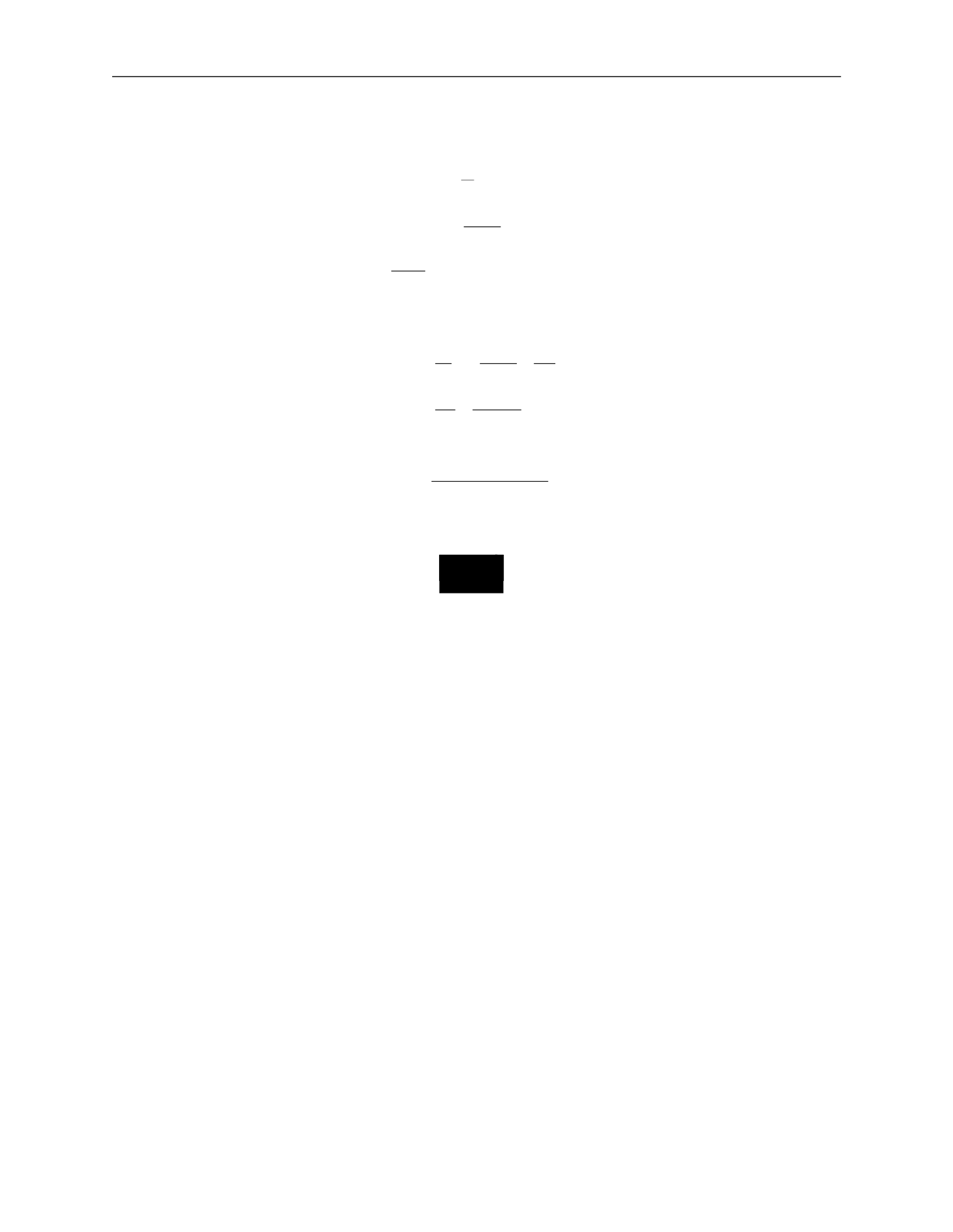
3.
MODELLING GALAXIES
38
v
·
Luminosity-velocity relations:
We can relate properties of a galaxy to observables through several equations:
R
θ
=
(apparent size)
d
L
F
=
4πd
2
(158)
v
2
=
GM .
R
Introducing surface brightness Σ
F
L
d
2
Σ =
=
θ
2
4πd
2
R
2
(159)
L
v
4
then
=
4π
·
G2M 2
v
4
L =
Σ4πG
2
(M/L)
2
.
(160)
If we assume, for a given class of galaxies, that the surface brightness and the mass-to-light
ratio are the same, then
.
(161)
This introduces two important relations.
The Tully-Fischer relation is used for spiral galaxies and relates the maximum velocity in
the rotation curve
v
max
, which can be measured from HII spectra, and the luminosity:
4
max
.
(162)
The Faber-Jackson relation is used for ellipticals and relates the velocity dispersion
σ
v
to the
luminosity:
L
∝
σ
4
.
(163)
Thus, we can get an estimate of the intrinsic luminosity of a galaxy be measuring stel-
lar velocities. The constant of proportionality is roughly
L
∗
/(220 km/s)
4
, where
L
∗
is the
characteristic galaxy luminosity.
3.J
Phase-space distribution function
We have described the individual orbits in a potential, but this is not sufficient to describe
galactic dynamics. We want information of the configuration of all particles. Each star is
described by its position
→
x
and velocity
→
v
,
and we need to know this for all stars, i.e. how
stars are distributed in the 6D phase space
(
→
x
,
→
v
)
.
We define a phase-space distribution function
f
(
→
x
,
→
v
,
t)d3
→
x
d
3
→
v
(164)
∝
L
∝
v

3.
MODELLING GALAXIES
39
∈
dt
as the probability that at time
t
, a randomly chosen star has
(
→
x
∗
,
→
v
∗
)
([
→
x
,
→
x
+
d
→
x
]
,
[
→
v
,
→
v
+
d
→
v])
.
This
means
that
the function must be normalized for all
t
, i.e.
∫
f
(
→
x
,
→
v
,
t)d
3
→
x
d
3
→
v
= 1 .
(165)
Collisionless
Boltzmann
equation
:
We want to describe the time evolution of
f
(
→
x
,
→
v
,
t)
. Since probability cannot be destroyed,
the 6D continuity equation must hold.
We define the 6D phase-space vector
then
w
→
=
(
→
x
,
→
v
)
(166)
∂f
+
∂
f
w
→
˙
=
0 .
(167)
∂t
∂w
→
This is the same form as the standard 3D continuity equation. We can rewrite this by
expanding out
w
→
and using velocity
→
v
=
→
x
˙
and acceleration
→
a
=
→
v
˙
:
0
= ∂f +
∂
f
w
→
˙
∂t
∂w
→
∂f
∂
=
+
∂t
∂
→
x
(
f
→
x
˙
) +
∂
(
f
→
v
˙
)
∂
→
v
(168)
∂f
∂
∂
=
+
(
f
→
v
)
+
f
(
−
∇
→
φ)
∂t
∂
→
x
∂
→
v
∂f
∂f
∂φ
∂f
=
∂t
+
→
v
∂
→
x
−
∂
→
x
∂
→
v
.
This gives us the collisionless Boltzmann equation (CBE):
.
(169)
Note that another way to see this is by writing out
df
= 0
and taking the limits
lim
→x
→∞
= 0
and
lim
→v
→∞
= 0
.
General Jeans equations:
A solution to the collisionless Boltzmann equation is difficult to obtain, so we instead study
moments of the CBE and the phase-space distribution.
Moments of the phase-space density give us some average quantities of the system.
a)
The first moment gives the density
n
of the system:
n
=
∫
f
d
3
→
v
.
(170)
∂t
−
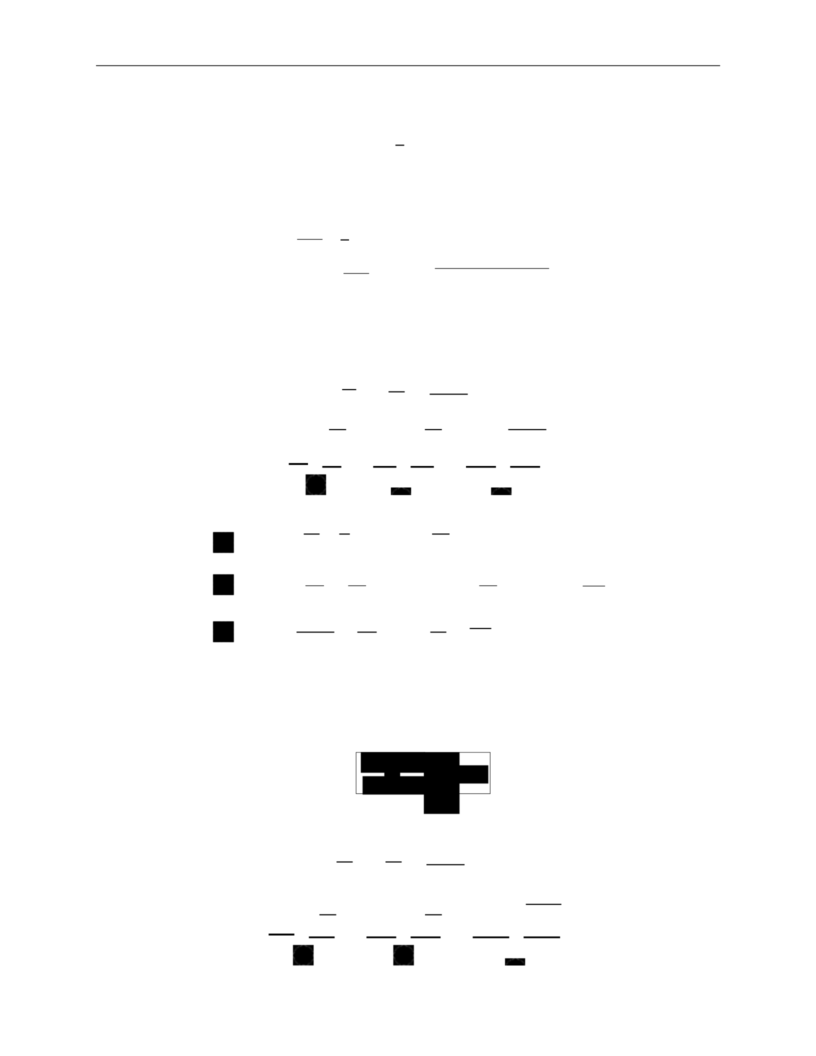
3.
MODELLING GALAXIES
40
ij
∫
—
∫
∫
∫
±∞
—
i
n
i
i
j
n
i
j
∂
→
x
∂
→
v
∂
→
x
∂
→
v
∂
→
x
→v=
−∞
j
∂t
j
∂
→
x
j
∂
→
x
∂
→
v
2
b)
The second moment gives the average velocity
v
¯
i
:
v
¯
=
1
∫
v
f
d
3
→
v
.
(171)
c)
The third moment gives the velocity dispersion
σ
2
:
v v
=
1
∫
v v
f
d
3
→
v
ij
=
v
i
v
j
−
v
¯
i
v
¯
j
=
(v
i
−
v
¯
i
)(
v
j
−
v
¯
j
)
.
We now examine moments of the collisionless Boltzmann equation more closely. We break
each integral into three terms to simplify each individually.
o)
First moment:
d
3
→
v
∂f
∂t
∂f
+
→
v
∂
→
x
∂φ
∂f
=
0
∂
→
x
∂
→
v
∫
d
3
→
v
∂f +
∫
d
3
→
v
→
v
∂f
−
∫
d
3
→
v
∂φ
∂f =
0 (173)
∂t
` ˛
1
¸ x
∂
→
x
` ˛
2
¸ x
∂
→
x
∂
→
v
` ˛
3
¸ x
:
d
3
→
v
∂f =
∂
∂t ∂t
d
3
→
v
f
=
∂n
∂t
:
d
3
→
v
→
v
∂f
∂
→
x
∂
=
∂
→
x
d3
→
v
→
v
f
=
∂
∂
→
x
n
→
v
¯
=
Σ
∂
∂x
i
(
n
v
¯
i
)
(174)
:
∫
d
3
→
v
∂φ
∂f
=
∂φ
∫
d
3
→
v
∂f
=
∂φ [f ]
→v=+
∞
=
0
For the third term, we used the fact that phase-space distribution goes to 0 at
for
physical systems.
This gives us the 3D continuity equation:
p)
Second moment:
.
(175)
∫
d
3
→
v
vj
∂f
∂f
+
→
v
∂t
∂
→
x
∂φ
∂f
=
0
∂
→
x
∂
→
v
∫
d
3
→
v
v
∂f +
∫
d
3
→
v
v
→
v
∂f
−
∫
d
3
→
v
v
∂φ
∂f
=
0
(176)
` ˛
1
¸ x ` ˛
2
¸ x ` ˛
3
¸ x
1
2
3
∂n ∂
∂t
0
σ
∫
i
(172)

3.
MODELLING GALAXIES
41
ij
Σ
∫
i
∂x
∂x
j
∂t
∂t
j
∂t
j
∂t
∂t
∂x
i
∂t
∂t
j
∂x
i
using the continuity equation ∂n
=
−
Σ
∂
(
n
v
¯
)
j
∂
→
x
i
∂x
i
∂x
i
j
i
i
∂x
ij
i
j
∂x
j
∂v
j
v
i
=
−∞
i
∂v
∂t
∂x
i
∂x
ij
i
j
∂x
i
`
i
i
ij
i
∂x
i
∂v
:
∫
d
3
→
v
v
∂f =
∂
∫
d
3
→
v
v
f =
∂
(
n
v
¯
) =
∂
n
v
¯
+
n
∂
v
¯
j
=
−
v
¯
Σ
∂
(
n
v
¯
) +
n
∂
v
¯
j
=
n
∂
v
¯
j
−
v
¯
Σ
∂
(
n
v
¯
)
∂t
∂x
i
i
to go from the first line to the second
:
∫
d
3
→
v
v
→
v
∂f
=
∫
d
3
→
v
v
Σ
v
∂f =
Σ
∂
∫
d
3
→
v
v v
f
= nv
j
v
i
`
= n
˛ ¸
σ
2
+
x
v
¯
i
v
¯
j
=
Σ
∂
n
σ
2
+
v
¯
v
¯
:
∫
d
3
→
v
v
∂φ
∂f
=
∫
d
3
→
v
v
Σ
∂φ
∂f
=
Σ
∂φ
∫
d
3
→
v
v
∂f
(177)
((k, l, i) are permutations of (1, 2, 3))
=
∂φ
dv
∂x
k
∫
dv
l
∫
dv
i
∂f
v
j
∂v
=
[v
f
]
˛
v
¸
i
=+
∞
−
x
∫
dv ∂v
j
f
= 0
−
∫
dv
i
δ
ij
f
=
−
Σ
∂φ
∫
dv
∫
dv
l
∫
dv
i
δ
ij
f
i
i
=
−
Σ
∂φ
∫
d
3
→
v
δ
f
i
i
∂φ
=
−
n∂x
j
Plugging each term back in, we get
n
∂
v
¯
j
−
v
¯
Σ
∂
(
n
v
¯
) +
Σ
∂
n
σ
2
+
v
¯
v
¯
+
n
∂φ
=
0
(178)
i
i
i
i
i
i
i
i
i
i
i
1
2
3
j
j
i
j
i
i
j
∂
→
x
∂
→
v
j
i
i
i
j
k

3.
MODELLING GALAXIES
42
Σ
v
¯
2
2
∂t
j
∂x
i
∂x
ij
i
∂x
i
i
j
∂x
j
=
(
n
v
¯
i
)
∂
x
v
¯
j
+
v
¯
j
∂x
(
n
v
¯
i
)
∂t
i
∂x
j
∂x
ij
∂x
—
1
Σ
∂(nσ
ij
) :
pressure
∂t
i
i
i
i
i
i
i
i
j
which we can rewrite
n
∂
v
¯
j
−
v
¯
Σ
∂
(
n
v
¯
)
+
Σ
∂
(nσ
2
)+
Σ
∂
(
n
v
¯
v
¯
)
+n
∂φ
=
0
`
Σ˛¸
∂
x
Σ
∂
(179)
where the two underlined terms cancel. This gives us
n
∂
v
¯
j
+
Σ
(
n
v
¯
)
∂
v
¯
+
Σ
∂
(nσ
2
) +
n
∂φ
=
0 .
(180)
This is the Jeans equation, often written
(181)
Each term can be physically interpreted:
∂
v
¯
j
∂t
∂
v
¯
j
i
∂x
: acceleration of fluid
: kinematic viscosity/shear
i
i
2
(182)
n
∂x
i
∂φ
−
∂x
j
: gravity
Jeans
equations
in
spherical
systems
:
We can convert to spherical coordinates and take velocity moments to give us the Jeans
equations in spherical coordinates. This is complicated!
To simplify, we take the radial Jeans equation and focus on steady-state symmetric systems.
Implications:
∂
=
0
since we have steady state
•
v
¯
r
=
0
otherwise we have net radial motion
•
v
¯
θ
=
v
¯
φ
=
0
or the symmetry is broken
•
σ
rφ
=
0
or the symmetry is broken
2
•
σ
φφ
≡
σ
or the symmetry is broken.
2
2
rθ
θθ
t
∂φ
1
∂t
•
=
σ
=
σ
i
i
i
i
i
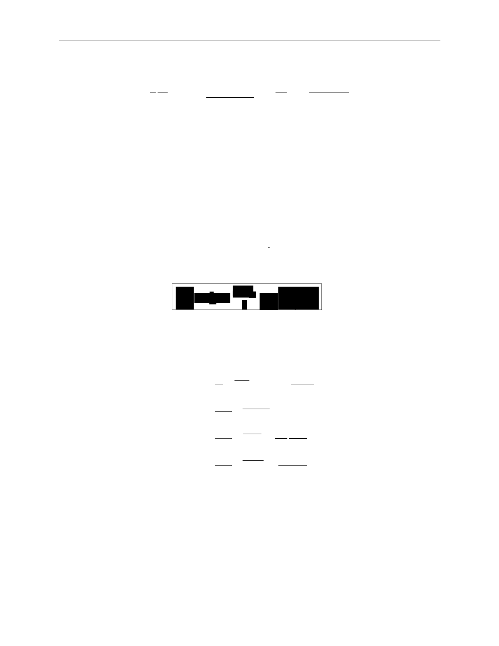
3.
MODELLING GALAXIES
43
2
2
2
2
t
t
t
— t
2
rr
rσ
rσ
rσ
rr
r
∂r
G
n
∂r
rr
—
dr
2
—
The simplified Jeans equation is:
1 ∂ 2(σ2
− σ ) ∂φ
GM (< r)
(nσ
2
) +
rr
t
=
−
=
−
(183)
where we’ve plugged in gravity as the force.
We have three limits we can look at:
•
σ
rr
•
σ
rr
•
σ
rr
σ
2
: nearly circular orbits
σ
2
: nearly radial orbits
= σ
2
: isotropic orbits
We define the anisotropy parameter:
σ
2
β
=
1
rr
(184)
which gives us a useful form of the Jeans equation for observations:
.
(185)
This depends only on radial components with uncertainty from
β
, assuming spherical sym-
metry and a steady-state system.
This can be simplified further to get mass estimates:
r2
1 ∂ 2 2βσ2
M (< r)
=
−
(nσ
)
+
2
=
−
rr
r
∂
(nσ
2
)
+
2β
G
2
=
rr
G
2
rr
r dn
+
n dr
rr
r
dσ
2
rr
+
2β
rr
(186)
2
=
rr
G
d ln n
+
d ln r
d ln σ2
rr
+
2β
d ln r
where the last line can be measured with observations.
Stability of stellar systems
The existence of equilibrium solutions to the collisionless Boltzmann equation does not assure
stability. Real stellar systems are subject to perturbations. What is important for stability?
1 ∂
2βσ2
σ
nσ
σ
n
∂r
r
2
r
∂r
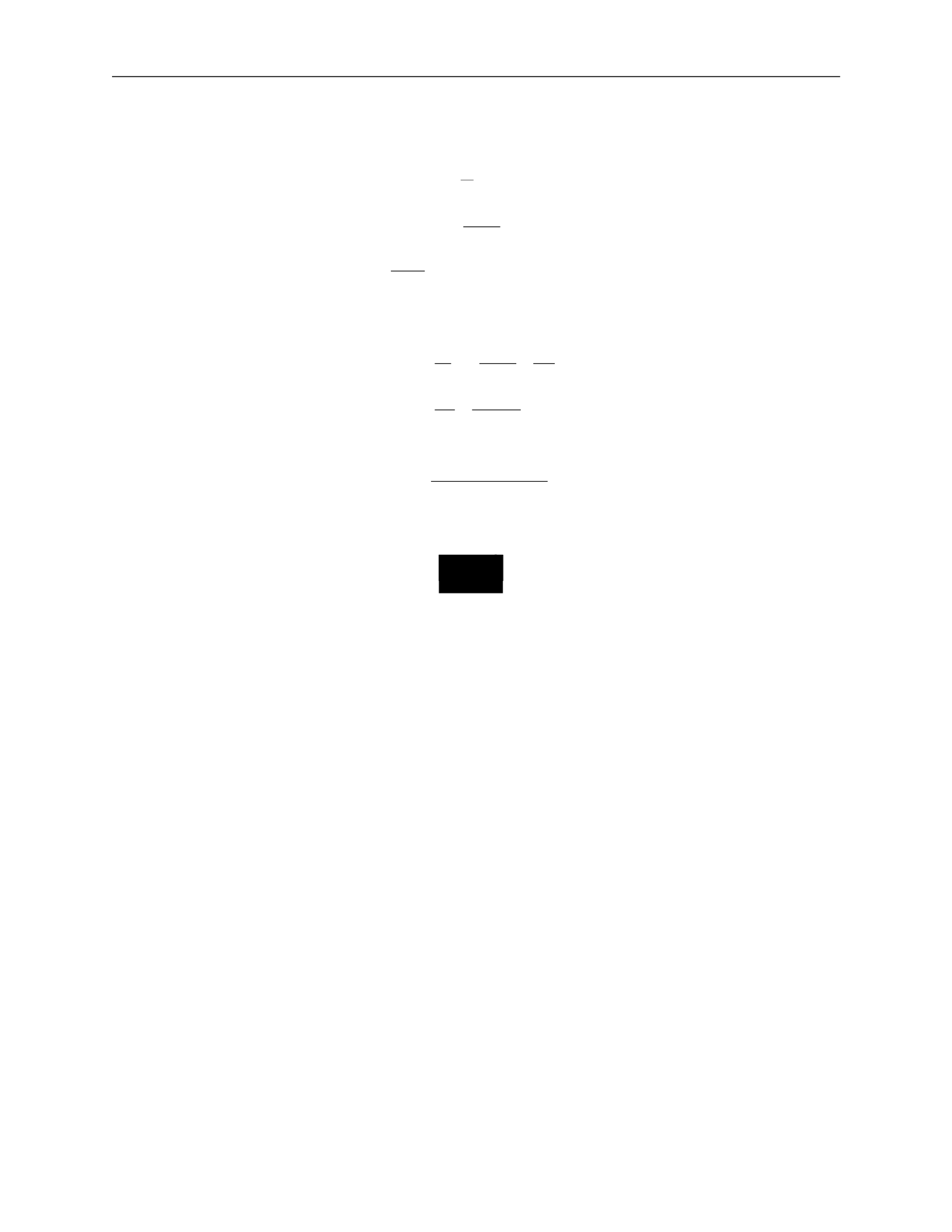
3.
MODELLING GALAXIES
38
v
·
Luminosity-velocity relations:
We can relate properties of a galaxy to observables through several equations:
R
θ
=
(apparent size)
d
L
F
=
4πd
2
(158)
v
2
=
GM .
R
Introducing surface brightness Σ
F
L
d
2
Σ =
=
θ
2
4πd
2
R
2
(159)
L
v
4
then
=
4π
·
G2M 2
v
4
L =
Σ4πG
2
(M/L)
2
.
(160)
If we assume, for a given class of galaxies, that the surface brightness and the mass-to-light
ratio are the same, then
.
(161)
This introduces two important relations.
The Tully-Fischer relation is used for spiral galaxies and relates the maximum velocity in
the rotation curve
v
max
, which can be measured from HII spectra, and the luminosity:
4
max
.
(162)
The Faber-Jackson relation is used for ellipticals and relates the velocity dispersion
σ
v
to the
luminosity:
L
∝
σ
4
.
(163)
Thus, we can get an estimate of the intrinsic luminosity of a galaxy be measuring stel-
lar velocities. The constant of proportionality is roughly
L
∗
/(220 km/s)
4
, where
L
∗
is the
characteristic galaxy luminosity.
3.K
Phase-space distribution function
We have described the individual orbits in a potential, but this is not sufficient to describe
galactic dynamics. We want information of the configuration of all particles. Each star is
described by its position
→
x
and velocity
→
v
,
and we need to know this for all stars, i.e. how
stars are distributed in the 6D phase space
(
→
x
,
→
v
)
.
We define a phase-space distribution function
f
(
→
x
,
→
v
,
t)d3
→
x
d
3
→
v
(164)
∝
L
∝
v

3.
MODELLING GALAXIES
39
∈
dt
as the probability that at time
t
, a randomly chosen star has
(
→
x
∗
,
→
v
∗
)
([
→
x
,
→
x
+
d
→
x
]
,
[
→
v
,
→
v
+
d
→
v])
.
This
means
that
the function must be normalized for all
t
, i.e.
∫
f
(
→
x
,
→
v
,
t)d
3
→
x
d
3
→
v
= 1 .
(165)
Collisionless
Boltzmann
equation
:
We want to describe the time evolution of
f
(
→
x
,
→
v
,
t)
. Since probability cannot be destroyed,
the 6D continuity equation must hold.
We define the 6D phase-space vector
then
w
→
=
(
→
x
,
→
v
)
(166)
∂f
+
∂
f
w
→
˙
=
0 .
(167)
∂t
∂w
→
This is the same form as the standard 3D continuity equation. We can rewrite this by
expanding out
w
→
and using velocity
→
v
=
→
x
˙
and acceleration
→
a
=
→
v
˙
:
0
= ∂f +
∂
f
w
→
˙
∂t
∂w
→
∂f
∂
=
+
∂t
∂
→
x
(
f
→
x
˙
) +
∂
(
f
→
v
˙
)
∂
→
v
(168)
∂f
∂
∂
=
+
(
f
→
v
)
+
f
(
−
∇
→
φ)
∂t
∂
→
x
∂
→
v
∂f
∂f
∂φ
∂f
=
∂t
+
→
v
∂
→
x
−
∂
→
x
∂
→
v
.
This gives us the collisionless Boltzmann equation (CBE):
.
(169)
Note that another way to see this is by writing out
df
= 0
and taking the limits
lim
→x
→∞
= 0
and
lim
→v
→∞
= 0
.
General Jeans equations:
A solution to the collisionless Boltzmann equation is difficult to obtain, so we instead study
moments of the CBE and the phase-space distribution.
Moments of the phase-space density give us some average quantities of the system.
a)
The first moment gives the density
n
of the system:
n
=
∫
f
d
3
→
v
.
(170)
∂t
−
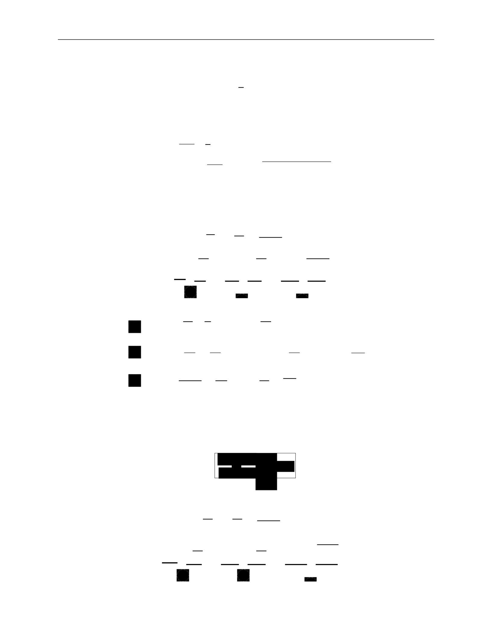
3.
MODELLING GALAXIES
40
ij
∫
—
∫
∫
∫
±∞
—
i
n
i
i
j
n
i
j
∂
→
x
∂
→
v
∂
→
x
∂
→
v
∂
→
x
→v=
−∞
j
∂t
j
∂
→
x
j
∂
→
x
∂
→
v
2
b)
The second moment gives the average velocity
v
¯
i
:
v
¯
=
1
∫
v
f
d
3
→
v
.
(171)
c)
The third moment gives the velocity dispersion
σ
2
:
v v
=
1
∫
v v
f
d
3
→
v
ij
=
v
i
v
j
−
v
¯
i
v
¯
j
=
(v
i
−
v
¯
i
)(
v
j
−
v
¯
j
)
.
We now examine moments of the collisionless Boltzmann equation more closely. We break
each integral into three terms to simplify each individually.
q)
First moment:
d
3
→
v
∂f
∂t
∂f
+
→
v
∂
→
x
∂φ
∂f
=
0
∂
→
x
∂
→
v
∫
d
3
→
v
∂f +
∫
d
3
→
v
→
v
∂f
−
∫
d
3
→
v
∂φ
∂f =
0 (173)
∂t
` ˛
1
¸ x
∂
→
x
` ˛
2
¸ x
∂
→
x
∂
→
v
` ˛
3
¸ x
:
d
3
→
v
∂f =
∂
∂t ∂t
d
3
→
v
f
=
∂n
∂t
:
d
3
→
v
→
v
∂f
∂
→
x
∂
=
∂
→
x
d3
→
v
→
v
f
=
∂
∂
→
x
n
→
v
¯
=
Σ
∂
∂x
i
(
n
v
¯
i
)
(174)
:
∫
d
3
→
v
∂φ
∂f
=
∂φ
∫
d
3
→
v
∂f
=
∂φ [f ]
→v=+
∞
=
0
For the third term, we used the fact that phase-space distribution goes to 0 at
for
physical systems.
This gives us the 3D continuity equation:
r)
Second moment:
.
(175)
∫
d
3
→
v
vj
∂f
∂f
+
→
v
∂t
∂
→
x
∂φ
∂f
=
0
∂
→
x
∂
→
v
∫
d
3
→
v
v
∂f +
∫
d
3
→
v
v
→
v
∂f
−
∫
d
3
→
v
v
∂φ
∂f
=
0
(176)
` ˛
1
¸ x ` ˛
2
¸ x ` ˛
3
¸ x
1
2
3
∂n ∂
∂t
0
σ
∫
i
(172)

3.
MODELLING GALAXIES
41
ij
Σ
∫
i
∂x
∂x
j
∂t
∂t
j
∂t
j
∂t
∂t
∂x
i
∂t
∂t
j
∂x
i
using the continuity equation ∂n
=
−
Σ
∂
(
n
v
¯
)
j
∂
→
x
i
∂x
i
∂x
i
j
i
i
∂x
ij
i
j
∂x
j
∂v
j
v
i
=
−∞
i
∂v
∂t
∂x
i
∂x
ij
i
j
∂x
i
`
i
i
ij
i
∂x
i
∂v
:
∫
d
3
→
v
v
∂f =
∂
∫
d
3
→
v
v
f =
∂
(
n
v
¯
) =
∂
n
v
¯
+
n
∂
v
¯
j
=
−
v
¯
Σ
∂
(
n
v
¯
) +
n
∂
v
¯
j
=
n
∂
v
¯
j
−
v
¯
Σ
∂
(
n
v
¯
)
∂t
∂x
i
i
to go from the first line to the second
:
∫
d
3
→
v
v
→
v
∂f
=
∫
d
3
→
v
v
Σ
v
∂f =
Σ
∂
∫
d
3
→
v
v v
f
= nv
j
v
i
`
= n
˛ ¸
σ
2
+
x
v
¯
i
v
¯
j
=
Σ
∂
n
σ
2
+
v
¯
v
¯
:
∫
d
3
→
v
v
∂φ
∂f
=
∫
d
3
→
v
v
Σ
∂φ
∂f
=
Σ
∂φ
∫
d
3
→
v
v
∂f
(177)
((k, l, i) are permutations of (1, 2, 3))
=
∂φ
dv
∂x
k
∫
dv
l
∫
dv
i
∂f
v
j
∂v
=
[v
f
]
˛
v
¸
i
=+
∞
−
x
∫
dv ∂v
j
f
= 0
−
∫
dv
i
δ
ij
f
=
−
Σ
∂φ
∫
dv
∫
dv
l
∫
dv
i
δ
ij
f
i
i
=
−
Σ
∂φ
∫
d
3
→
v
δ
f
i
i
∂φ
=
−
n∂x
j
Plugging each term back in, we get
n
∂
v
¯
j
−
v
¯
Σ
∂
(
n
v
¯
) +
Σ
∂
n
σ
2
+
v
¯
v
¯
+
n
∂φ
=
0
(178)
i
i
i
i
i
i
i
i
i
i
i
1
2
3
j
j
i
j
i
i
j
∂
→
x
∂
→
v
j
i
i
i
j
k

3.
MODELLING GALAXIES
42
Σ
v
¯
2
2
∂t
j
∂x
i
∂x
ij
i
∂x
i
i
j
∂x
j
=
(
n
v
¯
i
)
∂
x
v
¯
j
+
v
¯
j
∂x
(
n
v
¯
i
)
∂t
i
∂x
j
∂x
ij
∂x
—
1
Σ
∂(nσ
ij
) :
pressure
∂t
i
i
i
i
i
i
i
i
j
which we can rewrite
n
∂
v
¯
j
−
v
¯
Σ
∂
(
n
v
¯
)
+
Σ
∂
(nσ
2
)+
Σ
∂
(
n
v
¯
v
¯
)
+n
∂φ
=
0
`
Σ˛¸
∂
x
Σ
∂
(179)
where the two underlined terms cancel. This gives us
n
∂
v
¯
j
+
Σ
(
n
v
¯
)
∂
v
¯
+
Σ
∂
(nσ
2
) +
n
∂φ
=
0 .
(180)
This is the Jeans equation, often written
(181)
Each term can be physically interpreted:
∂
v
¯
j
∂t
∂
v
¯
j
i
∂x
: acceleration of fluid
: kinematic viscosity/shear
i
i
2
(182)
n
∂x
i
∂φ
−
∂x
j
: gravity
Jeans
equations
in
spherical
systems
:
We can convert to spherical coordinates and take velocity moments to give us the Jeans
equations in spherical coordinates. This is complicated!
To simplify, we take the radial Jeans equation and focus on steady-state symmetric systems.
Implications:
∂
=
0
since we have steady state
•
v
¯
r
=
0
otherwise we have net radial motion
•
v
¯
θ
=
v
¯
φ
=
0
or the symmetry is broken
•
σ
rφ
=
0
or the symmetry is broken
2
•
σ
φφ
≡
σ
or the symmetry is broken.
2
2
rθ
θθ
t
∂φ
1
∂t
•
=
σ
=
σ
i
i
i
i
i
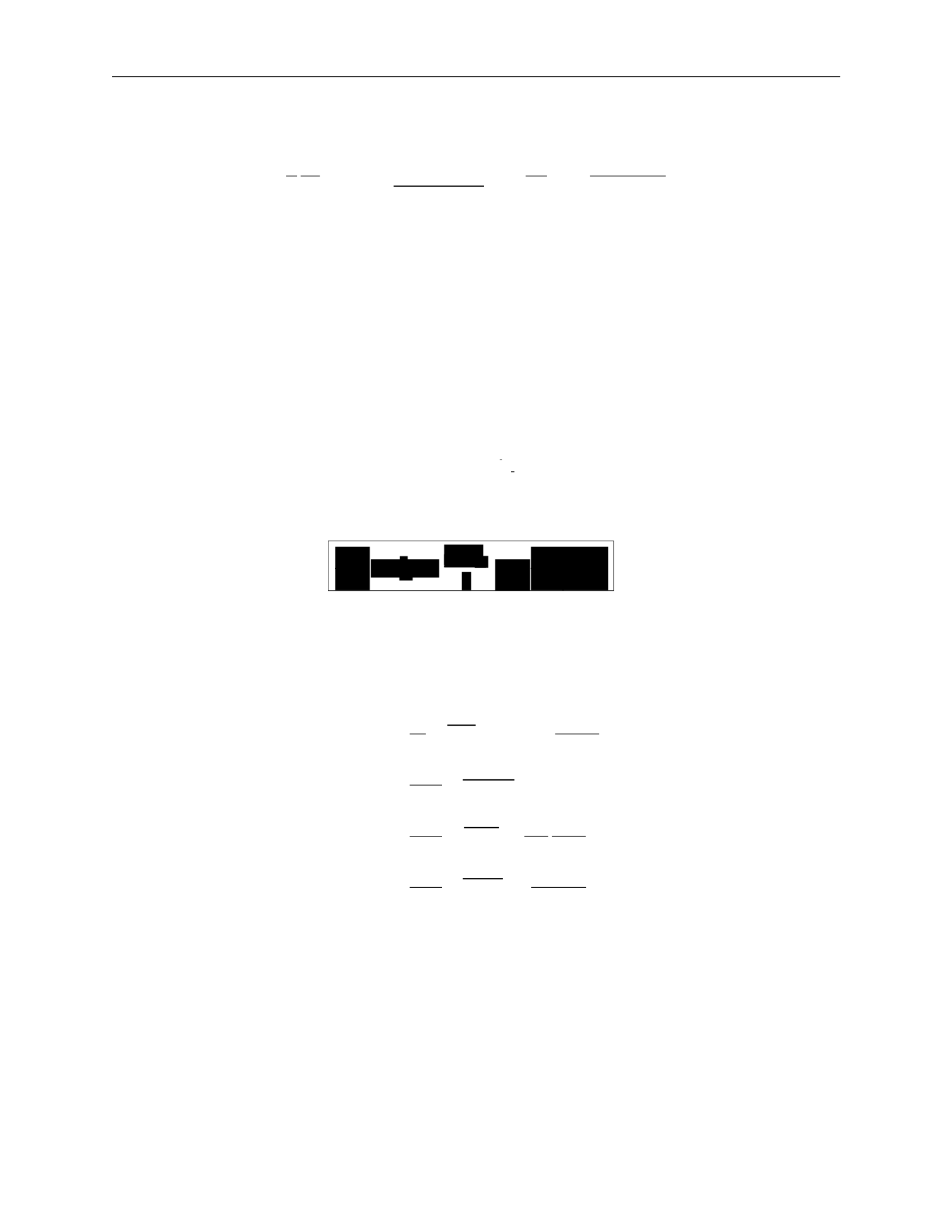
3.
MODELLING GALAXIES
43
2
2
2
2
t
t
t
— t
2
rr
rσ
rσ
rσ
rr
r
∂r
G
n
∂r
rr
—
dr
2
—
The simplified Jeans equation is:
1 ∂ 2(σ2
− σ ) ∂φ
GM (< r)
(nσ
2
) +
rr
t
=
−
=
−
(183)
where we’ve plugged in gravity as the force.
We have three limits we can look at:
•
σ
rr
•
σ
rr
•
σ
rr
σ
2
: nearly circular orbits
σ
2
: nearly radial orbits
= σ
2
: isotropic orbits
We define the anisotropy parameter:
σ
2
β
=
1
rr
(184)
which gives us a useful form of the Jeans equation for observations:
.
(185)
This depends only on radial components with uncertainty from
β
, assuming spherical sym-
metry and a steady-state system.
This can be simplified further to get mass estimates:
r2
1 ∂ 2 2βσ2
M (< r)
=
−
(nσ
)
+
2
=
−
rr
r
∂
(nσ
2
)
+
2β
G
2
=
rr
G
2
rr
r dn
+
n dr
rr
r
dσ
2
rr
+
2β
rr
(186)
2
=
rr
G
d ln n
+
d ln r
d ln σ2
rr
+
2β
d ln r
where the last line can be measured with observations.
Stability of stellar systems
The existence of equilibrium solutions to the collisionless Boltzmann equation does not assure stability.
Real stellar systems are subject to perturbations. What is important for stability?
1 ∂
2βσ2
σ
nσ
σ
n
∂r
r
2
r
∂r
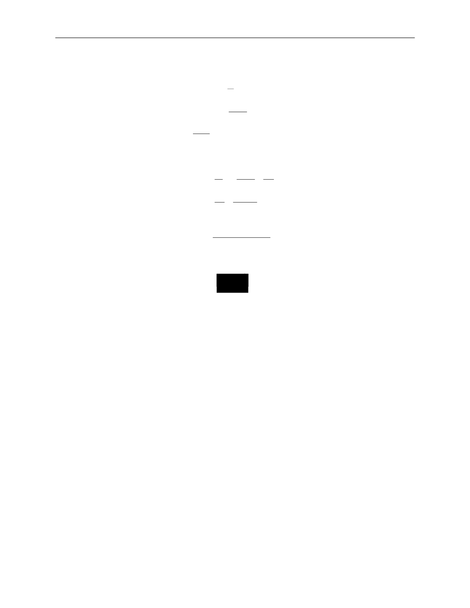
3.
MODELLING GALAXIES
38
v
·
Luminosity-velocity relations:
We can relate properties of a galaxy to observables through several equations:
R
θ
=
(apparent size)
d
L
F
=
4πd
2
(158)
v
2
=
GM .
R
Introducing surface brightness Σ
F
L
d
2
Σ =
=
θ
2
4πd
2
R
2
(159)
L
v
4
then
=
4π
·
G2M 2
v
4
L =
Σ4πG
2
(M/L)
2
.
(160)
If we assume, for a given class of galaxies, that the surface brightness and the mass-to-light
ratio are the same, then
.
(161)
This introduces two important relations.
The Tully-Fischer relation is used for spiral galaxies and relates the maximum velocity in
the rotation curve
v
max
, which can be measured from HII spectra, and the luminosity:
4
max
.
(162)
The Faber-Jackson relation is used for ellipticals and relates the velocity dispersion
σ
v
to the
luminosity:
L
∝
σ
4
.
(163)
Thus, we can get an estimate of the intrinsic luminosity of a galaxy be measuring stel-
lar velocities. The constant of proportionality is roughly
L
∗
/(220 km/s)
4
, where
L
∗
is the
characteristic galaxy luminosity.
3.L
Phase-space distribution function
We have described the individual orbits in a potential, but this is not sufficient to describe
galactic dynamics. We want information of the configuration of all particles. Each star is
described by its position
→
x
and velocity
→
v
,
and we need to know this for all stars, i.e. how
stars are distributed in the 6D phase space
(
→
x
,
→
v
)
.
We define a phase-space distribution function
f
(
→
x
,
→
v
,
t)d3
→
x
d
3
→
v
(164)
∝
L
∝
v

3.
MODELLING GALAXIES
39
∈
dt
as the probability that at time
t
, a randomly chosen star has
(
→
x
∗
,
→
v
∗
)
([
→
x
,
→
x
+
d
→
x
]
,
[
→
v
,
→
v
+
d
→
v])
.
This
means
that
the function must be normalized for all
t
, i.e.
∫
f
(
→
x
,
→
v
,
t)d
3
→
x
d
3
→
v
= 1 .
(165)
Collisionless
Boltzmann
equation
:
We want to describe the time evolution of
f
(
→
x
,
→
v
,
t)
. Since probability cannot be destroyed,
the 6D continuity equation must hold.
We define the 6D phase-space vector
then
w
→
=
(
→
x
,
→
v
)
(166)
∂f
+
∂
f
w
→
˙
=
0 .
(167)
∂t
∂w
→
This is the same form as the standard 3D continuity equation. We can rewrite this by
expanding out
w
→
and using velocity
→
v
=
→
x
˙
and acceleration
→
a
=
→
v
˙
:
0
= ∂f +
∂
f
w
→
˙
∂t
∂w
→
∂f
∂
=
+
∂t
∂
→
x
(
f
→
x
˙
) +
∂
(
f
→
v
˙
)
∂
→
v
(168)
∂f
∂
∂
=
+
(
f
→
v
)
+
f
(
−
∇
→
φ)
∂t
∂
→
x
∂
→
v
∂f
∂f
∂φ
∂f
=
∂t
+
→
v
∂
→
x
−
∂
→
x
∂
→
v
.
This gives us the collisionless Boltzmann equation (CBE):
.
(169)
Note that another way to see this is by writing out
df
= 0
and taking the limits
lim
→x
→∞
= 0
and
lim
→v
→∞
= 0
.
General Jeans equations:
A solution to the collisionless Boltzmann equation is difficult to obtain, so we instead study
moments of the CBE and the phase-space distribution.
Moments of the phase-space density give us some average quantities of the system.
a)
The first moment gives the density
n
of the system:
n
=
∫
f
d
3
→
v
.
(170)
∂t
−

3.
MODELLING GALAXIES
40
ij
∫
—
∫
∫
∫
±∞
—
i
n
i
i
j
n
i
j
∂
→
x
∂
→
v
∂
→
x
∂
→
v
∂
→
x
→v=
−∞
j
∂t
j
∂
→
x
j
∂
→
x
∂
→
v
2
b)
The second moment gives the average velocity
v
¯
i
:
v
¯
=
1
∫
v
f
d
3
→
v
.
(171)
c)
The third moment gives the velocity dispersion
σ
2
:
v v
=
1
∫
v v
f
d
3
→
v
ij
=
v
i
v
j
−
v
¯
i
v
¯
j
=
(v
i
−
v
¯
i
)(
v
j
−
v
¯
j
)
.
We now examine moments of the collisionless Boltzmann equation more closely. We break
each integral into three terms to simplify each individually.
s)
First moment:
d
3
→
v
∂f
∂t
∂f
+
→
v
∂
→
x
∂φ
∂f
=
0
∂
→
x
∂
→
v
∫
d
3
→
v
∂f +
∫
d
3
→
v
→
v
∂f
−
∫
d
3
→
v
∂φ
∂f =
0 (173)
∂t
` ˛
1
¸ x
∂
→
x
` ˛
2
¸ x
∂
→
x
∂
→
v
` ˛
3
¸ x
:
d
3
→
v
∂f =
∂
∂t ∂t
d
3
→
v
f
=
∂n
∂t
:
d
3
→
v
→
v
∂f
∂
→
x
∂
=
∂
→
x
d3
→
v
→
v
f
=
∂
∂
→
x
n
→
v
¯
=
Σ
∂
∂x
i
(
n
v
¯
i
)
(174)
:
∫
d
3
→
v
∂φ
∂f
=
∂φ
∫
d
3
→
v
∂f
=
∂φ [f ]
→v=+
∞
=
0
For the third term, we used the fact that phase-space distribution goes to 0 at
for
physical systems.
This gives us the 3D continuity equation:
t)
Second moment:
.
(175)
∫
d
3
→
v
vj
∂f
∂f
+
→
v
∂t
∂
→
x
∂φ
∂f
=
0
∂
→
x
∂
→
v
∫
d
3
→
v
v
∂f +
∫
d
3
→
v
v
→
v
∂f
−
∫
d
3
→
v
v
∂φ
∂f
=
0
(176)
` ˛
1
¸ x ` ˛
2
¸ x ` ˛
3
¸ x
1
2
3
∂n ∂
∂t
0
σ
∫
i
(172)

3.
MODELLING GALAXIES
41
ij
Σ
∫
i
∂x
∂x
j
∂t
∂t
j
∂t
j
∂t
∂t
∂x
i
∂t
∂t
j
∂x
i
using the continuity equation ∂n
=
−
Σ
∂
(
n
v
¯
)
j
∂
→
x
i
∂x
i
∂x
i
j
i
i
∂x
ij
i
j
∂x
j
∂v
j
v
i
=
−∞
i
∂v
∂t
∂x
i
∂x
ij
i
j
∂x
i
`
i
i
ij
i
∂x
i
∂v
:
∫
d
3
→
v
v
∂f =
∂
∫
d
3
→
v
v
f =
∂
(
n
v
¯
) =
∂
n
v
¯
+
n
∂
v
¯
j
=
−
v
¯
Σ
∂
(
n
v
¯
) +
n
∂
v
¯
j
=
n
∂
v
¯
j
−
v
¯
Σ
∂
(
n
v
¯
)
∂t
∂x
i
i
to go from the first line to the second
:
∫
d
3
→
v
v
→
v
∂f
=
∫
d
3
→
v
v
Σ
v
∂f =
Σ
∂
∫
d
3
→
v
v v
f
= nv
j
v
i
`
= n
˛ ¸
σ
2
+
x
v
¯
i
v
¯
j
=
Σ
∂
n
σ
2
+
v
¯
v
¯
:
∫
d
3
→
v
v
∂φ
∂f
=
∫
d
3
→
v
v
Σ
∂φ
∂f
=
Σ
∂φ
∫
d
3
→
v
v
∂f
(177)
((k, l, i) are permutations of (1, 2, 3))
=
∂φ
dv
∂x
k
∫
dv
l
∫
dv
i
∂f
v
j
∂v
=
[v
f
]
˛
v
¸
i
=+
∞
−
x
∫
dv ∂v
j
f
= 0
−
∫
dv
i
δ
ij
f
=
−
Σ
∂φ
∫
dv
∫
dv
l
∫
dv
i
δ
ij
f
i
i
=
−
Σ
∂φ
∫
d
3
→
v
δ
f
i
i
∂φ
=
−
n∂x
j
Plugging each term back in, we get
n
∂
v
¯
j
−
v
¯
Σ
∂
(
n
v
¯
) +
Σ
∂
n
σ
2
+
v
¯
v
¯
+
n
∂φ
=
0
(178)
i
i
i
i
i
i
i
i
i
i
i
1
2
3
j
j
i
j
i
i
j
∂
→
x
∂
→
v
j
i
i
i
j
k

3.
MODELLING GALAXIES
42
Σ
v
¯
2
2
∂t
j
∂x
i
∂x
ij
i
∂x
i
i
j
∂x
j
=
(
n
v
¯
i
)
∂
x
v
¯
j
+
v
¯
j
∂x
(
n
v
¯
i
)
∂t
i
∂x
j
∂x
ij
∂x
—
1
Σ
∂(nσ
ij
) :
pressure
∂t
i
i
i
i
i
i
i
i
j
which we can rewrite
n
∂
v
¯
j
−
v
¯
Σ
∂
(
n
v
¯
)
+
Σ
∂
(nσ
2
)+
Σ
∂
(
n
v
¯
v
¯
)
+n
∂φ
=
0
`
Σ˛¸
∂
x
Σ
∂
(179)
where the two underlined terms cancel. This gives us
n
∂
v
¯
j
+
Σ
(
n
v
¯
)
∂
v
¯
+
Σ
∂
(nσ
2
) +
n
∂φ
=
0 .
(180)
This is the Jeans equation, often written
(181)
Each term can be physically interpreted:
∂
v
¯
j
∂t
∂
v
¯
j
i
∂x
: acceleration of fluid
: kinematic viscosity/shear
i
i
2
(182)
n
∂x
i
∂φ
−
∂x
j
: gravity
Jeans
equations
in
spherical
systems
:
We can convert to spherical coordinates and take velocity moments to give us the Jeans
equations in spherical coordinates. This is complicated!
To simplify, we take the radial Jeans equation and focus on steady-state symmetric systems.
Implications:
∂
=
0
since we have steady state
•
v
¯
r
=
0
otherwise we have net radial motion
•
v
¯
θ
=
v
¯
φ
=
0
or the symmetry is broken
•
σ
rφ
=
0
or the symmetry is broken
2
•
σ
φφ
≡
σ
or the symmetry is broken.
2
2
rθ
θθ
t
∂φ
1
∂t
•
=
σ
=
σ
i
i
i
i
i
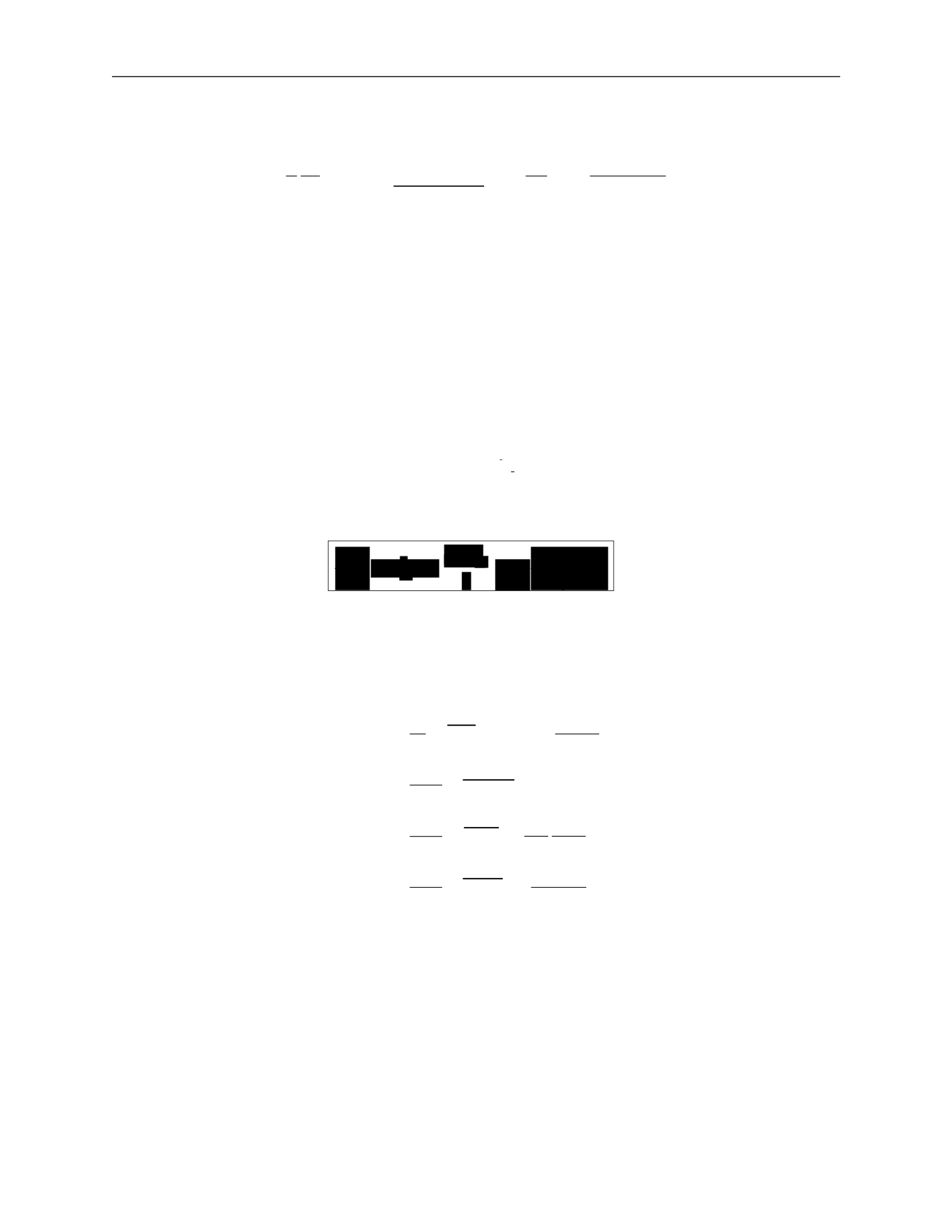
3.
MODELLING GALAXIES
43
2
2
2
2
t
t
t
— t
2
rr
rσ
rσ
rσ
rr
r
∂r
G
n
∂r
rr
—
dr
2
—
The simplified Jeans equation is:
1 ∂ 2(σ2
− σ ) ∂φ
GM (< r)
(nσ
2
) +
rr
t
=
−
=
−
(183)
where we’ve plugged in gravity as the force.
We have three limits we can look at:
•
σ
rr
•
σ
rr
•
σ
rr
σ
2
: nearly circular orbits
σ
2
: nearly radial orbits
= σ
2
: isotropic orbits
We define the anisotropy parameter:
σ
2
β
=
1
rr
(184)
which gives us a useful form of the Jeans equation for observations:
.
(185)
This depends only on radial components with uncertainty from
β
, assuming spherical sym-
metry and a steady-state system.
This can be simplified further to get mass estimates:
r2
1 ∂ 2 2βσ2
M (< r)
=
−
(nσ
)
+
2
=
−
rr
r
∂
(nσ
2
)
+
2β
G
2
=
rr
G
2
rr
r dn
+
n dr
rr
r
dσ
2
rr
+
2β
rr
(186)
2
=
rr
G
d ln n
+
d ln r
d ln σ2
rr
+
2β
d ln r
where the last line can be measured with observations.
Stability of stellar systems
The existence of equilibrium solutions to the collisionless Boltzmann equation does not assure
stability. Real stellar systems are subject to perturbations. What is important for stability?
1 ∂
2βσ2
σ
nσ
σ
n
∂r
r
2
r
∂r

3.
MODELLING GALAXIES
38
v
·
Luminosity-velocity relations:
We can relate properties of a galaxy to observables through several equations:
R
θ
=
(apparent size)
d
L
F
=
4πd
2
(158)
v
2
=
GM .
R
Introducing surface brightness Σ
F
L
d
2
Σ =
=
θ
2
4πd
2
R
2
(159)
L
v
4
then
=
4π
·
G2M 2
v
4
L =
Σ4πG
2
(M/L)
2
.
(160)
If we assume, for a given class of galaxies, that the surface brightness and the mass-to-light
ratio are the same, then
.
(161)
This introduces two important relations.
The Tully-Fischer relation is used for spiral galaxies and relates the maximum velocity in
the rotation curve
v
max
, which can be measured from HII spectra, and the luminosity:
4
max
.
(162)
The Faber-Jackson relation is used for ellipticals and relates the velocity dispersion
σ
v
to the
luminosity:
L
∝
σ
4
.
(163)
Thus, we can get an estimate of the intrinsic luminosity of a galaxy be measuring stel-
lar velocities. The constant of proportionality is roughly
L
∗
/(220 km/s)
4
, where
L
∗
is the
characteristic galaxy luminosity.
3.M
Phase-space distribution function
We have described the individual orbits in a potential, but this is not sufficient to describe
galactic dynamics. We want information of the configuration of all particles. Each star is
described by its position
→
x
and velocity
→
v
,
and we need to know this for all stars, i.e. how
stars are distributed in the 6D phase space
(
→
x
,
→
v
)
.
We define a phase-space distribution function
f
(
→
x
,
→
v
,
t)d3
→
x
d
3
→
v
(164)
∝
L
∝
v

3.
MODELLING GALAXIES
39
∈
dt
as the probability that at time
t
, a randomly chosen star has
(
→
x
∗
,
→
v
∗
)
([
→
x
,
→
x
+
d
→
x
]
,
[
→
v
,
→
v
+
d
→
v])
.
This
means
that
the function must be normalized for all
t
, i.e.
∫
f
(
→
x
,
→
v
,
t)d
3
→
x
d
3
→
v
= 1 .
(165)
Collisionless
Boltzmann
equation
:
We want to describe the time evolution of
f
(
→
x
,
→
v
,
t)
. Since probability cannot be destroyed,
the 6D continuity equation must hold.
We define the 6D phase-space vector
then
w
→
=
(
→
x
,
→
v
)
(166)
∂f
+
∂
f
w
→
˙
=
0 .
(167)
∂t
∂w
→
This is the same form as the standard 3D continuity equation. We can rewrite this by
expanding out
w
→
and using velocity
→
v
=
→
x
˙
and acceleration
→
a
=
→
v
˙
:
0
= ∂f +
∂
f
w
→
˙
∂t
∂w
→
∂f
∂
=
+
∂t
∂
→
x
(
f
→
x
˙
) +
∂
(
f
→
v
˙
)
∂
→
v
(168)
∂f
∂
∂
=
+
(
f
→
v
)
+
f
(
−
∇
→
φ)
∂t
∂
→
x
∂
→
v
∂f
∂f
∂φ
∂f
=
∂t
+
→
v
∂
→
x
−
∂
→
x
∂
→
v
.
This gives us the collisionless Boltzmann equation (CBE):
.
(169)
Note that another way to see this is by writing out
df
= 0
and taking the limits
lim
→x
→∞
= 0
and
lim
→v
→∞
= 0
.
General Jeans equations:
A solution to the collisionless Boltzmann equation is difficult to obtain, so we instead study
moments of the CBE and the phase-space distribution.
Moments of the phase-space density give us some average quantities of the system.
a)
The first moment gives the density
n
of the system:
n
=
∫
f
d
3
→
v
.
(170)
∂t
−
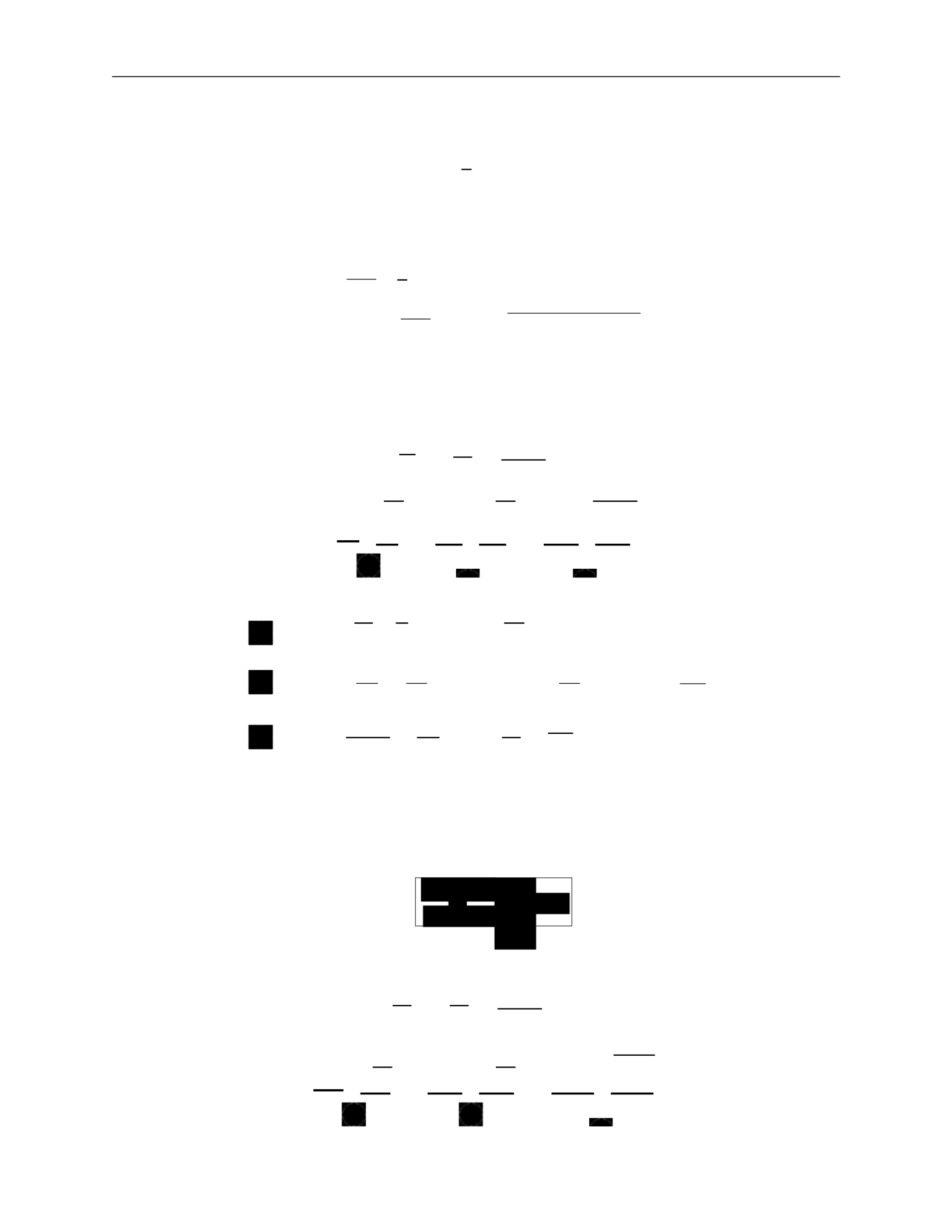
3.
MODELLING GALAXIES
40
ij
∫
—
∫
∫
∫
±∞
—
i
n
i
i
j
n
i
j
∂
→
x
∂
→
v
∂
→
x
∂
→
v
∂
→
x
→v=
−∞
j
∂t
j
∂
→
x
j
∂
→
x
∂
→
v
2
b)
The second moment gives the average velocity
v
¯
i
:
v
¯
=
1
∫
v
f
d
3
→
v
.
(171)
c)
The third moment gives the velocity dispersion
σ
2
:
v v
=
1
∫
v v
f
d
3
→
v
ij
=
v
i
v
j
−
v
¯
i
v
¯
j
=
(v
i
−
v
¯
i
)(
v
j
−
v
¯
j
)
.
We now examine moments of the collisionless Boltzmann equation more closely. We break
each integral into three terms to simplify each individually.
u)
First moment:
d
3
→
v
∂f
∂t
∂f
+
→
v
∂
→
x
∂φ
∂f
=
0
∂
→
x
∂
→
v
∫
d
3
→
v
∂f +
∫
d
3
→
v
→
v
∂f
−
∫
d
3
→
v
∂φ
∂f =
0 (173)
∂t
` ˛
1
¸ x
∂
→
x
` ˛
2
¸ x
∂
→
x
∂
→
v
` ˛
3
¸ x
:
d
3
→
v
∂f =
∂
∂t ∂t
d
3
→
v
f
=
∂n
∂t
:
d
3
→
v
→
v
∂f
∂
→
x
∂
=
∂
→
x
d3
→
v
→
v
f
=
∂
∂
→
x
n
→
v
¯
=
Σ
∂
∂x
i
(
n
v
¯
i
)
(174)
:
∫
d
3
→
v
∂φ
∂f
=
∂φ
∫
d
3
→
v
∂f
=
∂φ [f ]
→v=+
∞
=
0
For the third term, we used the fact that phase-space distribution goes to 0 at
for
physical systems.
This gives us the 3D continuity equation:
v)
Second moment:
.
(175)
∫
d
3
→
v
vj
∂f
∂f
+
→
v
∂t
∂
→
x
∂φ
∂f
=
0
∂
→
x
∂
→
v
∫
d
3
→
v
v
∂f +
∫
d
3
→
v
v
→
v
∂f
−
∫
d
3
→
v
v
∂φ
∂f
=
0
(176)
` ˛
1
¸ x ` ˛
2
¸ x ` ˛
3
¸ x
1
2
3
∂n ∂
∂t
0
σ
∫
i
(172)

3.
MODELLING GALAXIES
41
ij
Σ
∫
i
∂x
∂x
j
∂t
∂t
j
∂t
j
∂t
∂t
∂x
i
∂t
∂t
j
∂x
i
using the continuity equation ∂n
=
−
Σ
∂
(
n
v
¯
)
j
∂
→
x
i
∂x
i
∂x
i
j
i
i
∂x
ij
i
j
∂x
j
∂v
j
v
i
=
−∞
i
∂v
∂t
∂x
i
∂x
ij
i
j
∂x
i
`
i
i
ij
i
∂x
i
∂v
:
∫
d
3
→
v
v
∂f =
∂
∫
d
3
→
v
v
f =
∂
(
n
v
¯
) =
∂
n
v
¯
+
n
∂
v
¯
j
=
−
v
¯
Σ
∂
(
n
v
¯
) +
n
∂
v
¯
j
=
n
∂
v
¯
j
−
v
¯
Σ
∂
(
n
v
¯
)
∂t
∂x
i
i
to go from the first line to the second
:
∫
d
3
→
v
v
→
v
∂f
=
∫
d
3
→
v
v
Σ
v
∂f =
Σ
∂
∫
d
3
→
v
v v
f
= nv
j
v
i
`
= n
˛ ¸
σ
2
+
x
v
¯
i
v
¯
j
=
Σ
∂
n
σ
2
+
v
¯
v
¯
:
∫
d
3
→
v
v
∂φ
∂f
=
∫
d
3
→
v
v
Σ
∂φ
∂f
=
Σ
∂φ
∫
d
3
→
v
v
∂f
(177)
((k, l, i) are permutations of (1, 2, 3))
=
∂φ
dv
∂x
k
∫
dv
l
∫
dv
i
∂f
v
j
∂v
=
[v
f
]
˛
v
¸
i
=+
∞
−
x
∫
dv ∂v
j
f
= 0
−
∫
dv
i
δ
ij
f
=
−
Σ
∂φ
∫
dv
∫
dv
l
∫
dv
i
δ
ij
f
i
i
=
−
Σ
∂φ
∫
d
3
→
v
δ
f
i
i
∂φ
=
−
n∂x
j
Plugging each term back in, we get
n
∂
v
¯
j
−
v
¯
Σ
∂
(
n
v
¯
) +
Σ
∂
n
σ
2
+
v
¯
v
¯
+
n
∂φ
=
0
(178)
i
i
i
i
i
i
i
i
i
i
i
1
2
3
j
j
i
j
i
i
j
∂
→
x
∂
→
v
j
i
i
i
j
k

3.
MODELLING GALAXIES
42
Σ
v
¯
2
2
∂t
j
∂x
i
∂x
ij
i
∂x
i
i
j
∂x
j
=
(
n
v
¯
i
)
∂
x
v
¯
j
+
v
¯
j
∂x
(
n
v
¯
i
)
∂t
i
∂x
j
∂x
ij
∂x
—
1
Σ
∂(nσ
ij
) :
pressure
∂t
i
i
i
i
i
i
i
i
j
which we can rewrite
n
∂
v
¯
j
−
v
¯
Σ
∂
(
n
v
¯
)
+
Σ
∂
(nσ
2
)+
Σ
∂
(
n
v
¯
v
¯
)
+n
∂φ
=
0
`
Σ˛¸
∂
x
Σ
∂
(179)
where the two underlined terms cancel. This gives us
n
∂
v
¯
j
+
Σ
(
n
v
¯
)
∂
v
¯
+
Σ
∂
(nσ
2
) +
n
∂φ
=
0 .
(180)
This is the Jeans equation, often written
(181)
Each term can be physically interpreted:
∂
v
¯
j
∂t
∂
v
¯
j
i
∂x
: acceleration of fluid
: kinematic viscosity/shear
i
i
2
(182)
n
∂x
i
∂φ
−
∂x
j
: gravity
Jeans
equations
in
spherical
systems
:
We can convert to spherical coordinates and take velocity moments to give us the Jeans
equations in spherical coordinates. This is complicated!
To simplify, we take the radial Jeans equation and focus on steady-state symmetric systems.
Implications:
∂
=
0
since we have steady state
•
v
¯
r
=
0
otherwise we have net radial motion
•
v
¯
θ
=
v
¯
φ
=
0
or the symmetry is broken
•
σ
rφ
=
0
or the symmetry is broken
2
•
σ
φφ
≡
σ
or the symmetry is broken.
2
2
rθ
θθ
t
∂φ
1
∂t
•
=
σ
=
σ
i
i
i
i
i
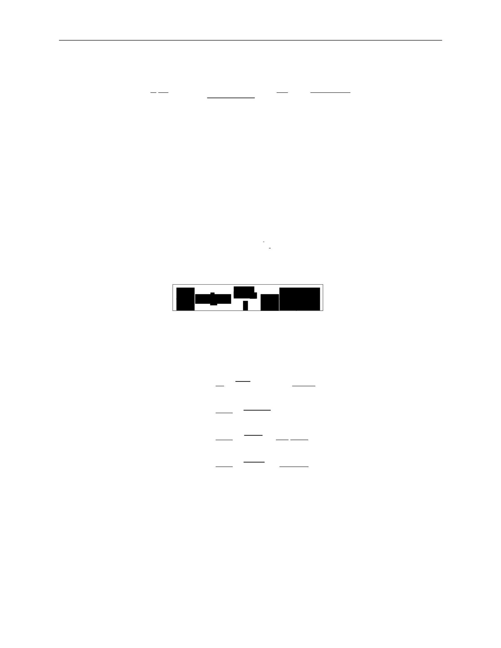
3.
MODELLING GALAXIES
43
2
2
2
2
t
t
t
— t
2
rr
rσ
rσ
rσ
rr
r
∂r
G
n
∂r
rr
—
dr
2
—
The simplified Jeans equation is:
1 ∂ 2(σ2
− σ ) ∂φ
GM (< r)
(nσ
2
) +
rr
t
=
−
=
−
(183)
where we’ve plugged in gravity as the force.
We have three limits we can look at:
•
σ
rr
•
σ
rr
•
σ
rr
σ
2
: nearly circular orbits
σ
2
: nearly radial orbits
= σ
2
: isotropic orbits
We define the anisotropy parameter:
σ
2
β
=
1
rr
(184)
which gives us a useful form of the Jeans equation for observations:
.
(185)
This depends only on radial components with uncertainty from
β
, assuming spherical sym-
metry and a steady-state system.
This can be simplified further to get mass estimates:
r2
1 ∂ 2 2βσ2
M (< r)
=
−
(nσ
)
+
2
=
−
rr
r
∂
(nσ
2
)
+
2β
G
2
=
rr
G
2
rr
r dn
+
n dr
rr
r
dσ
2
rr
+
2β
rr
(186)
2
=
rr
G
d ln n
+
d ln r
d ln σ2
rr
+
2β
d ln r
where the last line can be measured with observations.
Stability of stellar systems
The existence of equilibrium solutions to the collisionless Boltzmann equation does not assure stability.
Real stellar systems are subject to perturbations. What is important for stability?
1 ∂
2βσ2
σ
nσ
σ
n
∂r
r
2
r
∂r
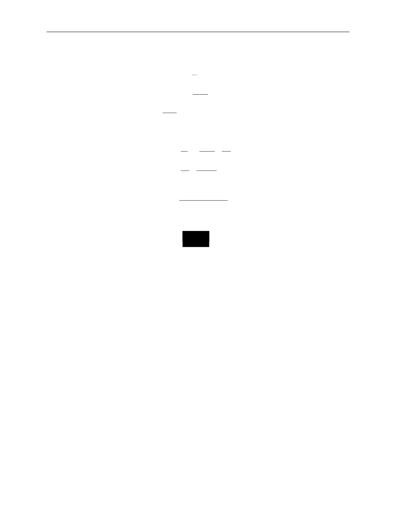
3.
MODELLING GALAXIES
38
v
·
Luminosity-velocity relations:
We can relate properties of a galaxy to observables through several equations:
R
θ
=
(apparent size)
d
L
F
=
4πd
2
(158)
v
2
=
GM .
R
Introducing surface brightness Σ
F
L
d
2
Σ =
=
θ
2
4πd
2
R
2
(159)
L
v
4
then
=
4π
·
G2M 2
v
4
L =
Σ4πG
2
(M/L)
2
.
(160)
If we assume, for a given class of galaxies, that the surface brightness and the mass-to-light
ratio are the same, then
.
(161)
This introduces two important relations.
The Tully-Fischer relation is used for spiral galaxies and relates the maximum velocity in
the rotation curve
v
max
, which can be measured from HII spectra, and the luminosity:
4
max
.
(162)
The Faber-Jackson relation is used for ellipticals and relates the velocity dispersion
σ
v
to the
luminosity:
L
∝
σ
4
.
(163)
Thus, we can get an estimate of the intrinsic luminosity of a galaxy be measuring stel-
lar velocities. The constant of proportionality is roughly
L
∗
/(220 km/s)
4
, where
L
∗
is the
characteristic galaxy luminosity.
3.N
Phase-space distribution function
We have described the individual orbits in a potential, but this is not sufficient to describe
galactic dynamics. We want information of the configuration of all particles. Each star is
described by its position
→
x
and velocity
→
v
,
and we need to know this for all stars, i.e. how
stars are distributed in the 6D phase space
(
→
x
,
→
v
)
.
We define a phase-space distribution function
f
(
→
x
,
→
v
,
t)d3
→
x
d
3
→
v
(164)
∝
L
∝
v
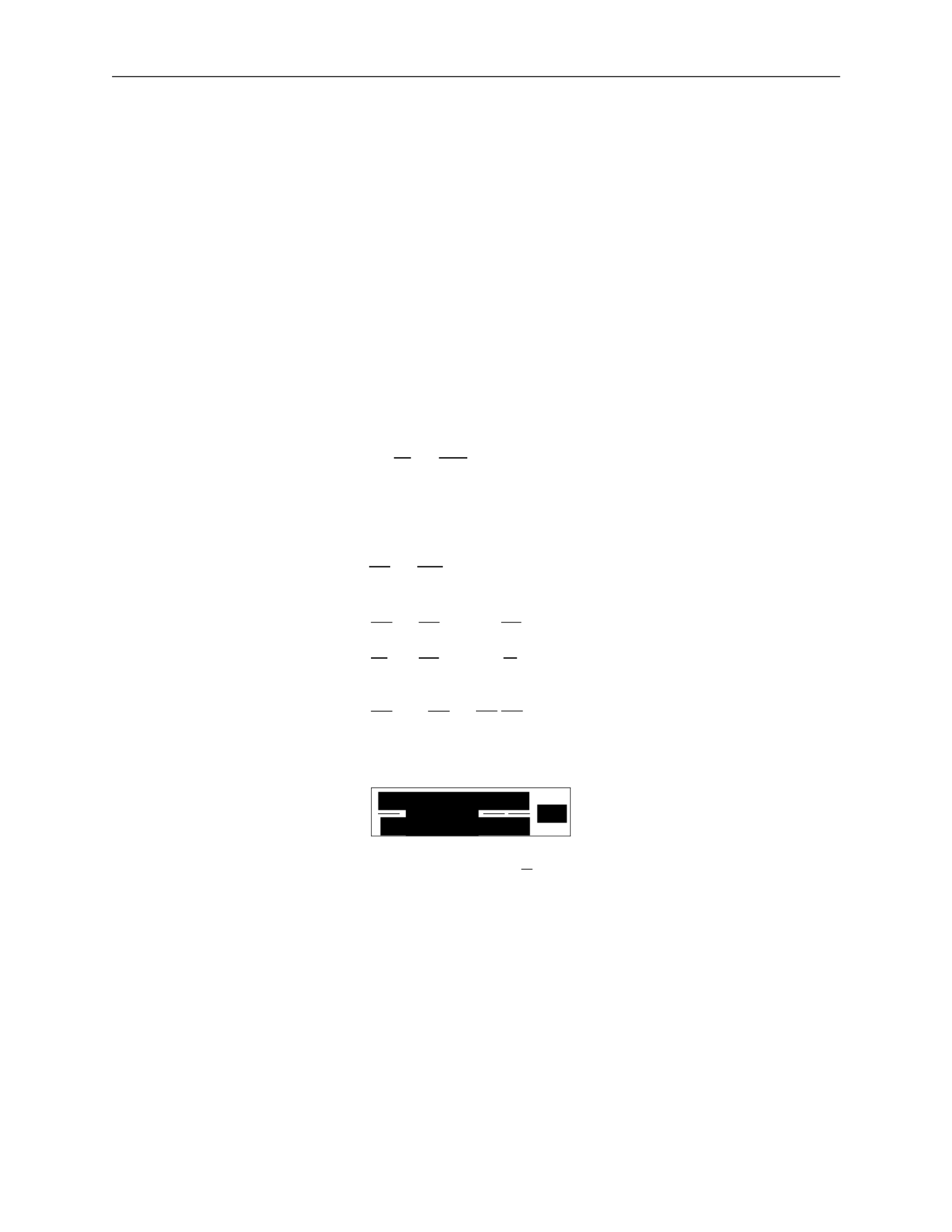
3.
MODELLING GALAXIES
39
∈
dt
as the probability that at time
t
, a randomly chosen star has
(
→
x
∗
,
→
v
∗
)
([
→
x
,
→
x
+
d
→
x
]
,
[
→
v
,
→
v
+
d
→
v])
.
This
means
that
the function must be normalized for all
t
, i.e.
∫
f
(
→
x
,
→
v
,
t)d
3
→
x
d
3
→
v
= 1 .
(165)
Collisionless
Boltzmann
equation
:
We want to describe the time evolution of
f
(
→
x
,
→
v
,
t)
. Since probability cannot be destroyed,
the 6D continuity equation must hold.
We define the 6D phase-space vector
then
w
→
=
(
→
x
,
→
v
)
(166)
∂f
+
∂
f
w
→
˙
=
0 .
(167)
∂t
∂w
→
This is the same form as the standard 3D continuity equation. We can rewrite this by
expanding out
w
→
and using velocity
→
v
=
→
x
˙
and acceleration
→
a
=
→
v
˙
:
0
= ∂f +
∂
f
w
→
˙
∂t
∂w
→
∂f
∂
=
+
∂t
∂
→
x
(
f
→
x
˙
) +
∂
(
f
→
v
˙
)
∂
→
v
(168)
∂f
∂
∂
=
+
(
f
→
v
)
+
f
(
−
∇
→
φ)
∂t
∂
→
x
∂
→
v
∂f
∂f
∂φ
∂f
=
∂t
+
→
v
∂
→
x
−
∂
→
x
∂
→
v
.
This gives us the collisionless Boltzmann equation (CBE):
.
(169)
Note that another way to see this is by writing out
df
= 0
and taking the limits
lim
→x
→∞
= 0
and
lim
→v
→∞
= 0
.
General Jeans equations:
A solution to the collisionless Boltzmann equation is difficult to obtain, so we instead study
moments of the CBE and the phase-space distribution.
Moments of the phase-space density give us some average quantities of the system.
a)
The first moment gives the density
n
of the system:
n
=
∫
f
d
3
→
v
.
(170)
∂t
−
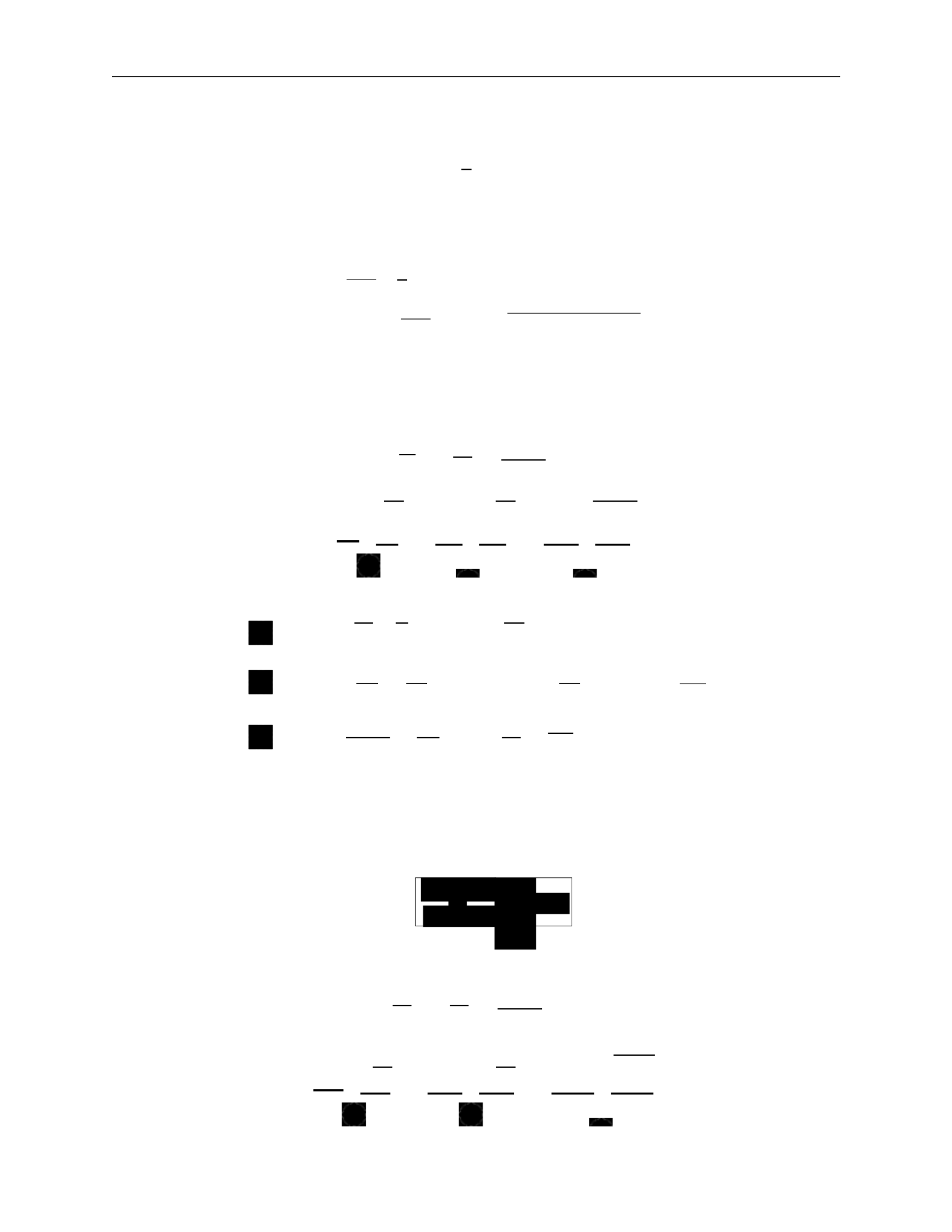
3.
MODELLING GALAXIES
40
ij
∫
—
∫
∫
∫
±∞
—
i
n
i
i
j
n
i
j
∂
→
x
∂
→
v
∂
→
x
∂
→
v
∂
→
x
→v=
−∞
j
∂t
j
∂
→
x
j
∂
→
x
∂
→
v
2
b)
The second moment gives the average velocity
v
¯
i
:
v
¯
=
1
∫
v
f
d
3
→
v
.
(171)
c)
The third moment gives the velocity dispersion
σ
2
:
v v
=
1
∫
v v
f
d
3
→
v
ij
=
v
i
v
j
−
v
¯
i
v
¯
j
=
(v
i
−
v
¯
i
)(
v
j
−
v
¯
j
)
.
We now examine moments of the collisionless Boltzmann equation more closely. We break
each integral into three terms to simplify each individually.
w)
First moment:
d
3
→
v
∂f
∂t
∂f
+
→
v
∂
→
x
∂φ
∂f
=
0
∂
→
x
∂
→
v
∫
d
3
→
v
∂f +
∫
d
3
→
v
→
v
∂f
−
∫
d
3
→
v
∂φ
∂f =
0 (173)
∂t
` ˛
1
¸ x
∂
→
x
` ˛
2
¸ x
∂
→
x
∂
→
v
` ˛
3
¸ x
:
d
3
→
v
∂f =
∂
∂t ∂t
d
3
→
v
f
=
∂n
∂t
:
d
3
→
v
→
v
∂f
∂
→
x
∂
=
∂
→
x
d3
→
v
→
v
f
=
∂
∂
→
x
n
→
v
¯
=
Σ
∂
∂x
i
(
n
v
¯
i
)
(174)
:
∫
d
3
→
v
∂φ
∂f
=
∂φ
∫
d
3
→
v
∂f
=
∂φ [f ]
→v=+
∞
=
0
For the third term, we used the fact that phase-space distribution goes to 0 at
for
physical systems.
This gives us the 3D continuity equation:
x)
Second moment:
.
(175)
∫
d
3
→
v
vj
∂f
∂f
+
→
v
∂t
∂
→
x
∂φ
∂f
=
0
∂
→
x
∂
→
v
∫
d
3
→
v
v
∂f +
∫
d
3
→
v
v
→
v
∂f
−
∫
d
3
→
v
v
∂φ
∂f
=
0
(176)
` ˛
1
¸ x ` ˛
2
¸ x ` ˛
3
¸ x
1
2
3
∂n ∂
∂t
0
σ
∫
i
(172)

3.
MODELLING GALAXIES
41
ij
Σ
∫
i
∂x
∂x
j
∂t
∂t
j
∂t
j
∂t
∂t
∂x
i
∂t
∂t
j
∂x
i
using the continuity equation ∂n
=
−
Σ
∂
(
n
v
¯
)
j
∂
→
x
i
∂x
i
∂x
i
j
i
i
∂x
ij
i
j
∂x
j
∂v
j
v
i
=
−∞
i
∂v
∂t
∂x
i
∂x
ij
i
j
∂x
i
`
i
i
ij
i
∂x
i
∂v
:
∫
d
3
→
v
v
∂f =
∂
∫
d
3
→
v
v
f =
∂
(
n
v
¯
) =
∂
n
v
¯
+
n
∂
v
¯
j
=
−
v
¯
Σ
∂
(
n
v
¯
) +
n
∂
v
¯
j
=
n
∂
v
¯
j
−
v
¯
Σ
∂
(
n
v
¯
)
∂t
∂x
i
i
to go from the first line to the second
:
∫
d
3
→
v
v
→
v
∂f
=
∫
d
3
→
v
v
Σ
v
∂f =
Σ
∂
∫
d
3
→
v
v v
f
= nv
j
v
i
`
= n
˛ ¸
σ
2
+
x
v
¯
i
v
¯
j
=
Σ
∂
n
σ
2
+
v
¯
v
¯
:
∫
d
3
→
v
v
∂φ
∂f
=
∫
d
3
→
v
v
Σ
∂φ
∂f
=
Σ
∂φ
∫
d
3
→
v
v
∂f
(177)
((k, l, i) are permutations of (1, 2, 3))
=
∂φ
dv
∂x
k
∫
dv
l
∫
dv
i
∂f
v
j
∂v
=
[v
f
]
˛
v
¸
i
=+
∞
−
x
∫
dv ∂v
j
f
= 0
−
∫
dv
i
δ
ij
f
=
−
Σ
∂φ
∫
dv
∫
dv
l
∫
dv
i
δ
ij
f
i
i
=
−
Σ
∂φ
∫
d
3
→
v
δ
f
i
i
∂φ
=
−
n∂x
j
Plugging each term back in, we get
n
∂
v
¯
j
−
v
¯
Σ
∂
(
n
v
¯
) +
Σ
∂
n
σ
2
+
v
¯
v
¯
+
n
∂φ
=
0
(178)
i
i
i
i
i
i
i
i
i
i
i
1
2
3
j
j
i
j
i
i
j
∂
→
x
∂
→
v
j
i
i
i
j
k

3.
MODELLING GALAXIES
42
Σ
v
¯
2
2
∂t
j
∂x
i
∂x
ij
i
∂x
i
i
j
∂x
j
=
(
n
v
¯
i
)
∂
x
v
¯
j
+
v
¯
j
∂x
(
n
v
¯
i
)
∂t
i
∂x
j
∂x
ij
∂x
—
1
Σ
∂(nσ
ij
) :
pressure
∂t
i
i
i
i
i
i
i
i
j
which we can rewrite
n
∂
v
¯
j
−
v
¯
Σ
∂
(
n
v
¯
)
+
Σ
∂
(nσ
2
)+
Σ
∂
(
n
v
¯
v
¯
)
+n
∂φ
=
0
`
Σ˛¸
∂
x
Σ
∂
(179)
where the two underlined terms cancel. This gives us
n
∂
v
¯
j
+
Σ
(
n
v
¯
)
∂
v
¯
+
Σ
∂
(nσ
2
) +
n
∂φ
=
0 .
(180)
This is the Jeans equation, often written
(181)
Each term can be physically interpreted:
∂
v
¯
j
∂t
∂
v
¯
j
i
∂x
: acceleration of fluid
: kinematic viscosity/shear
i
i
2
(182)
n
∂x
i
∂φ
−
∂x
j
: gravity
Jeans
equations
in
spherical
systems
:
We can convert to spherical coordinates and take velocity moments to give us the Jeans
equations in spherical coordinates. This is complicated!
To simplify, we take the radial Jeans equation and focus on steady-state symmetric systems.
Implications:
∂
=
0
since we have steady state
•
v
¯
r
=
0
otherwise we have net radial motion
•
v
¯
θ
=
v
¯
φ
=
0
or the symmetry is broken
•
σ
rφ
=
0
or the symmetry is broken
2
•
σ
φφ
≡
σ
or the symmetry is broken.
2
2
rθ
θθ
t
∂φ
1
∂t
•
=
σ
=
σ
i
i
i
i
i
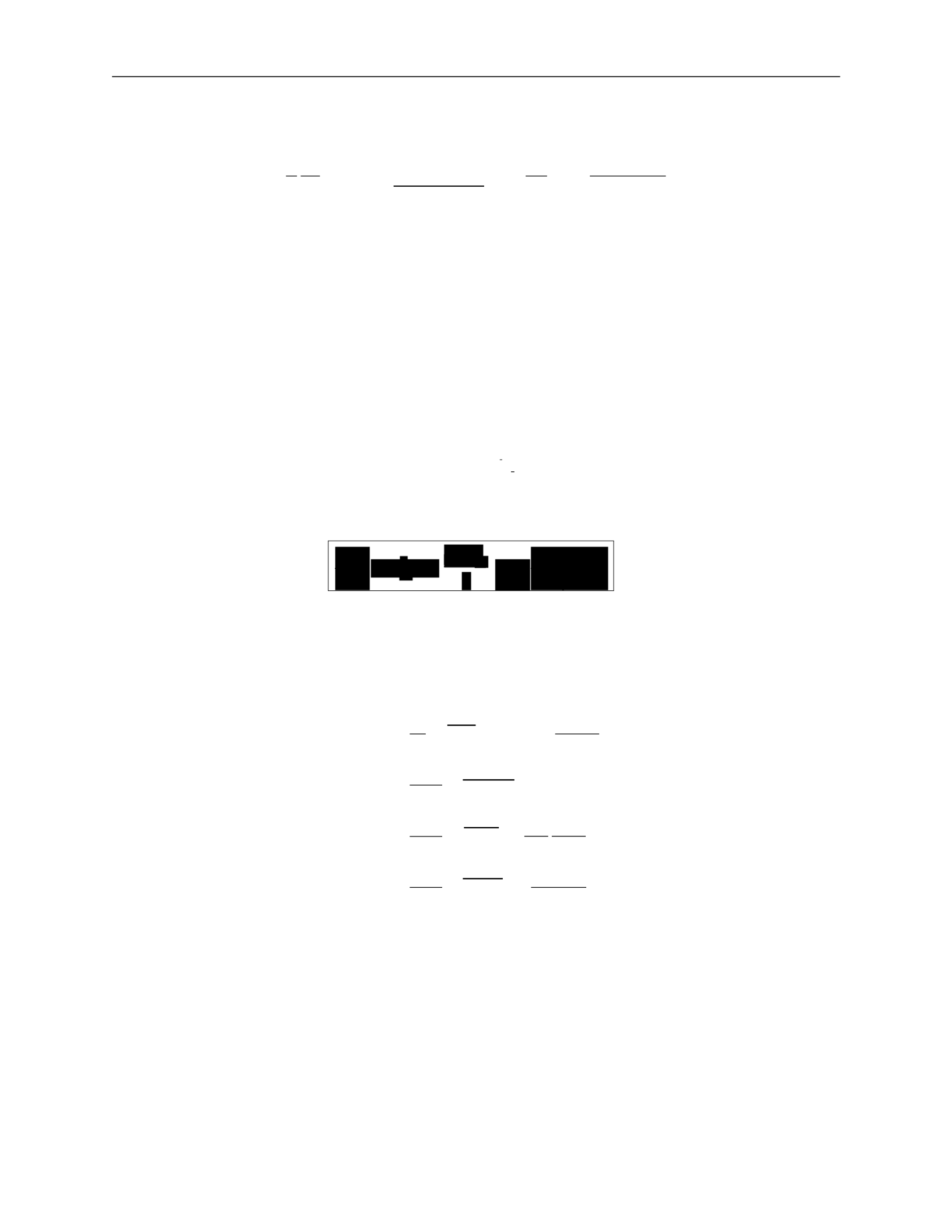
3.
MODELLING GALAXIES
43
2
2
2
2
t
t
t
— t
2
rr
rσ
rσ
rσ
rr
r
∂r
G
n
∂r
rr
—
dr
2
—
The simplified Jeans equation is:
1 ∂ 2(σ2
− σ ) ∂φ
GM (< r)
(nσ
2
) +
rr
t
=
−
=
−
(183)
where we’ve plugged in gravity as the force.
We have three limits we can look at:
•
σ
rr
•
σ
rr
•
σ
rr
σ
2
: nearly circular orbits
σ
2
: nearly radial orbits
= σ
2
: isotropic orbits
We define the anisotropy parameter:
σ
2
β
=
1
rr
(184)
which gives us a useful form of the Jeans equation for observations:
.
(185)
This depends only on radial components with uncertainty from
β
, assuming spherical sym-
metry and a steady-state system.
This can be simplified further to get mass estimates:
r2
1 ∂ 2 2βσ2
M (< r)
=
−
(nσ
)
+
2
=
−
rr
r
∂
(nσ
2
)
+
2β
G
2
=
rr
G
2
rr
r dn
+
n dr
rr
r
dσ
2
rr
+
2β
rr
(186)
2
=
rr
G
d ln n
+
d ln r
d ln σ2
rr
+
2β
d ln r
where the last line can be measured with observations.
Stability of stellar systems
The existence of equilibrium solutions to the collisionless Boltzmann equation does not assure
stability. Real stellar systems are subject to perturbations. What is important for stability?
1 ∂
2βσ2
σ
nσ
σ
n
∂r
r
2
r
∂r
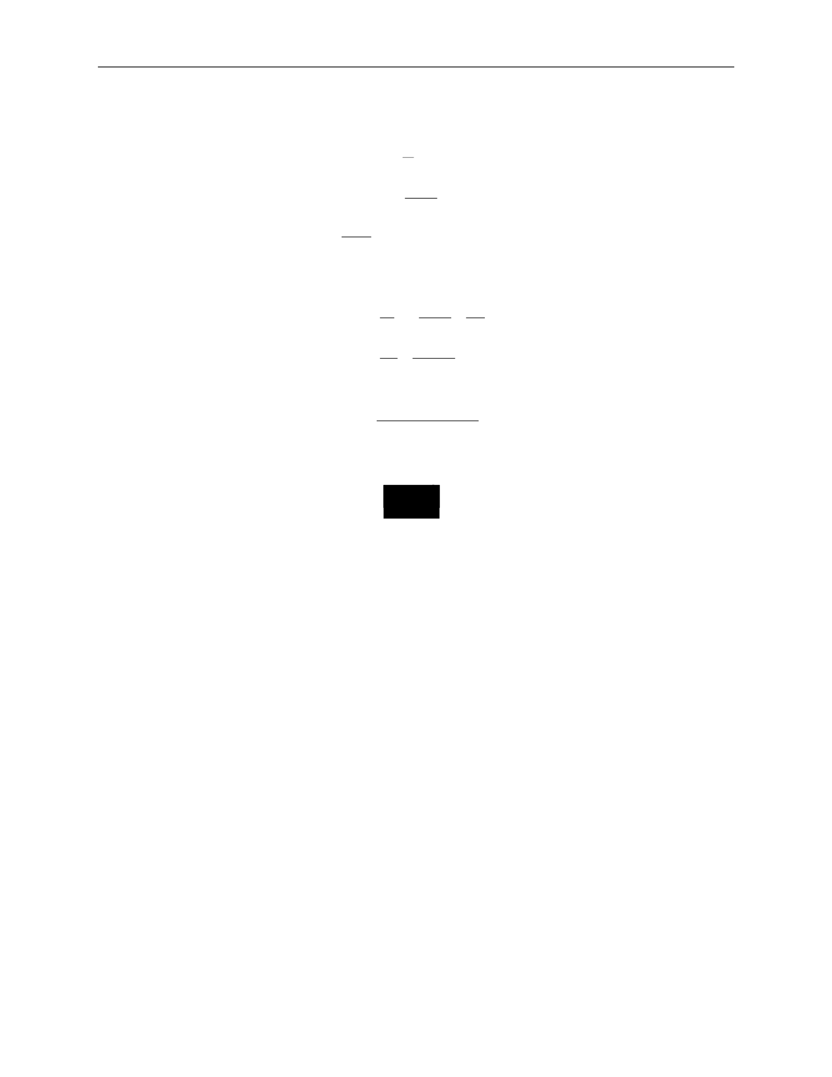
3.
MODELLING GALAXIES
38
v
·
Luminosity-velocity relations:
We can relate properties of a galaxy to observables through several equations:
R
θ
=
(apparent size)
d
L
F
=
4πd
2
(158)
v
2
=
GM .
R
Introducing surface brightness Σ
F
L
d
2
Σ =
=
θ
2
4πd
2
R
2
(159)
L
v
4
then
=
4π
·
G2M 2
v
4
L =
Σ4πG
2
(M/L)
2
.
(160)
If we assume, for a given class of galaxies, that the surface brightness and the mass-to-light
ratio are the same, then
.
(161)
This introduces two important relations.
The Tully-Fischer relation is used for spiral galaxies and relates the maximum velocity in
the rotation curve
v
max
, which can be measured from HII spectra, and the luminosity:
4
max
.
(162)
The Faber-Jackson relation is used for ellipticals and relates the velocity dispersion
σ
v
to the
luminosity:
L
∝
σ
4
.
(163)
Thus, we can get an estimate of the intrinsic luminosity of a galaxy be measuring stel-
lar velocities. The constant of proportionality is roughly
L
∗
/(220 km/s)
4
, where
L
∗
is the
characteristic galaxy luminosity.
3.O
Phase-space distribution function
We have described the individual orbits in a potential, but this is not sufficient to describe
galactic dynamics. We want information of the configuration of all particles. Each star is
described by its position
→
x
and velocity
→
v
,
and we need to know this for all stars, i.e. how
stars are distributed in the 6D phase space
(
→
x
,
→
v
)
.
We define a phase-space distribution function
f
(
→
x
,
→
v
,
t)d3
→
x
d
3
→
v
(164)
∝
L
∝
v
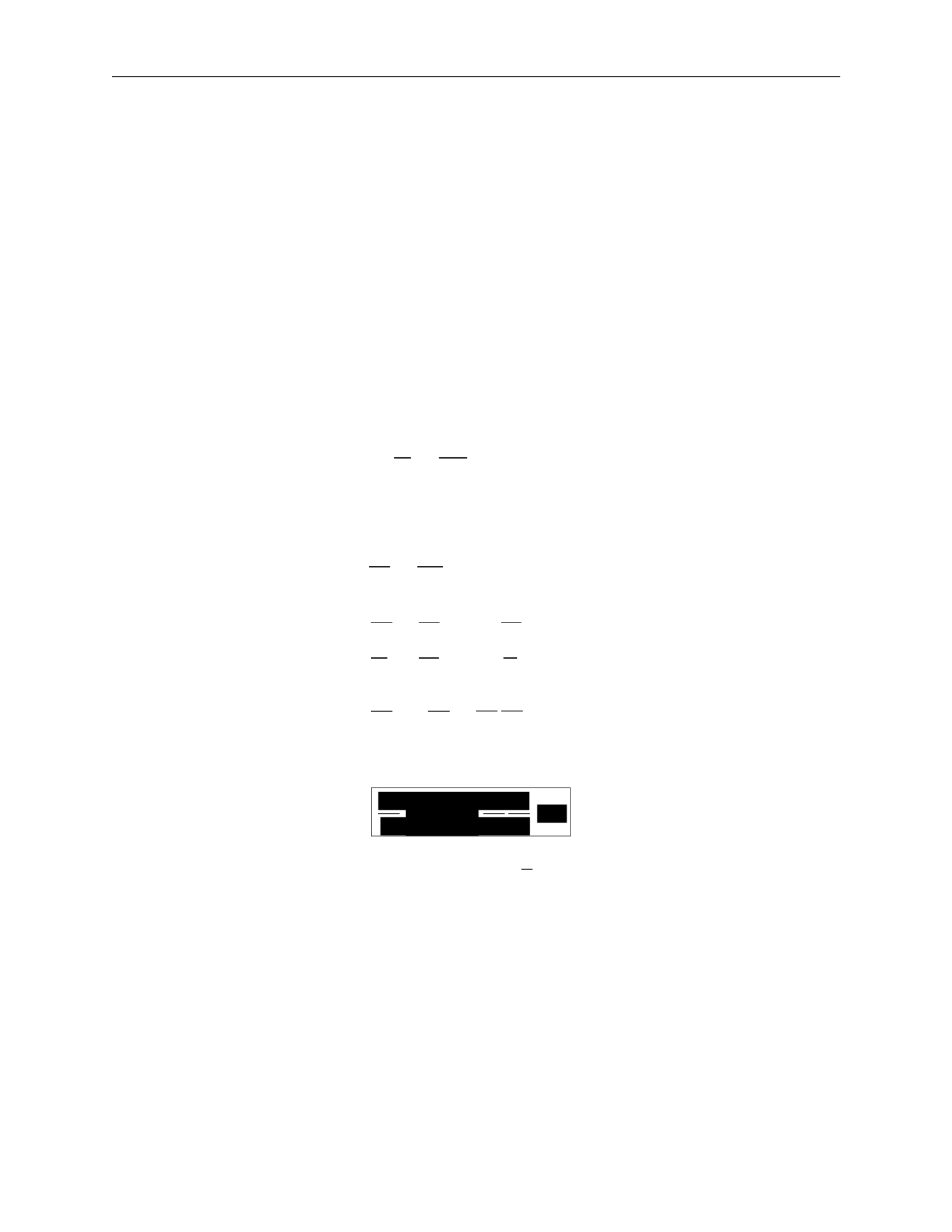
3.
MODELLING GALAXIES
39
∈
dt
as the probability that at time
t
, a randomly chosen star has
(
→
x
∗
,
→
v
∗
)
([
→
x
,
→
x
+
d
→
x
]
,
[
→
v
,
→
v
+
d
→
v])
.
This
means
that
the function must be normalized for all
t
, i.e.
∫
f
(
→
x
,
→
v
,
t)d
3
→
x
d
3
→
v
= 1 .
(165)
Collisionless
Boltzmann
equation
:
We want to describe the time evolution of
f
(
→
x
,
→
v
,
t)
. Since probability cannot be destroyed,
the 6D continuity equation must hold.
We define the 6D phase-space vector
then
w
→
=
(
→
x
,
→
v
)
(166)
∂f
+
∂
f
w
→
˙
=
0 .
(167)
∂t
∂w
→
This is the same form as the standard 3D continuity equation. We can rewrite this by
expanding out
w
→
and using velocity
→
v
=
→
x
˙
and acceleration
→
a
=
→
v
˙
:
0
= ∂f +
∂
f
w
→
˙
∂t
∂w
→
∂f
∂
=
+
∂t
∂
→
x
(
f
→
x
˙
) +
∂
(
f
→
v
˙
)
∂
→
v
(168)
∂f
∂
∂
=
+
(
f
→
v
)
+
f
(
−
∇
→
φ)
∂t
∂
→
x
∂
→
v
∂f
∂f
∂φ
∂f
=
∂t
+
→
v
∂
→
x
−
∂
→
x
∂
→
v
.
This gives us the collisionless Boltzmann equation (CBE):
.
(169)
Note that another way to see this is by writing out
df
= 0
and taking the limits
lim
→x
→∞
= 0
and
lim
→v
→∞
= 0
.
General Jeans equations:
A solution to the collisionless Boltzmann equation is difficult to obtain, so we instead study
moments of the CBE and the phase-space distribution.
Moments of the phase-space density give us some average quantities of the system.
a)
The first moment gives the density
n
of the system:
n
=
∫
f
d
3
→
v
.
(170)
∂t
−

3.
MODELLING GALAXIES
40
ij
∫
—
∫
∫
∫
±∞
—
i
n
i
i
j
n
i
j
∂
→
x
∂
→
v
∂
→
x
∂
→
v
∂
→
x
→v=
−∞
j
∂t
j
∂
→
x
j
∂
→
x
∂
→
v
2
b)
The second moment gives the average velocity
v
¯
i
:
v
¯
=
1
∫
v
f
d
3
→
v
.
(171)
c)
The third moment gives the velocity dispersion
σ
2
:
v v
=
1
∫
v v
f
d
3
→
v
ij
=
v
i
v
j
−
v
¯
i
v
¯
j
=
(v
i
−
v
¯
i
)(
v
j
−
v
¯
j
)
.
We now examine moments of the collisionless Boltzmann equation more closely. We break
each integral into three terms to simplify each individually.
y)
First moment:
d
3
→
v
∂f
∂t
∂f
+
→
v
∂
→
x
∂φ
∂f
=
0
∂
→
x
∂
→
v
∫
d
3
→
v
∂f +
∫
d
3
→
v
→
v
∂f
−
∫
d
3
→
v
∂φ
∂f =
0 (173)
∂t
` ˛
1
¸ x
∂
→
x
` ˛
2
¸ x
∂
→
x
∂
→
v
` ˛
3
¸ x
:
d
3
→
v
∂f =
∂
∂t ∂t
d
3
→
v
f
=
∂n
∂t
:
d
3
→
v
→
v
∂f
∂
→
x
∂
=
∂
→
x
d3
→
v
→
v
f
=
∂
∂
→
x
n
→
v
¯
=
Σ
∂
∂x
i
(
n
v
¯
i
)
(174)
:
∫
d
3
→
v
∂φ
∂f
=
∂φ
∫
d
3
→
v
∂f
=
∂φ [f ]
→v=+
∞
=
0
For the third term, we used the fact that phase-space distribution goes to 0 at
for
physical systems.
This gives us the 3D continuity equation:
z)
Second moment:
.
(175)
∫
d
3
→
v
vj
∂f
∂f
+
→
v
∂t
∂
→
x
∂φ
∂f
=
0
∂
→
x
∂
→
v
∫
d
3
→
v
v
∂f +
∫
d
3
→
v
v
→
v
∂f
−
∫
d
3
→
v
v
∂φ
∂f
=
0
(176)
` ˛
1
¸ x ` ˛
2
¸ x ` ˛
3
¸ x
1
2
3
∂n ∂
∂t
0
σ
∫
i
(172)

3.
MODELLING GALAXIES
41
ij
Σ
∫
i
∂x
∂x
j
∂t
∂t
j
∂t
j
∂t
∂t
∂x
i
∂t
∂t
j
∂x
i
using the continuity equation ∂n
=
−
Σ
∂
(
n
v
¯
)
j
∂
→
x
i
∂x
i
∂x
i
j
i
i
∂x
ij
i
j
∂x
j
∂v
j
v
i
=
−∞
i
∂v
∂t
∂x
i
∂x
ij
i
j
∂x
i
`
i
i
ij
i
∂x
i
∂v
:
∫
d
3
→
v
v
∂f =
∂
∫
d
3
→
v
v
f =
∂
(
n
v
¯
) =
∂
n
v
¯
+
n
∂
v
¯
j
=
−
v
¯
Σ
∂
(
n
v
¯
) +
n
∂
v
¯
j
=
n
∂
v
¯
j
−
v
¯
Σ
∂
(
n
v
¯
)
∂t
∂x
i
i
to go from the first line to the second
:
∫
d
3
→
v
v
→
v
∂f
=
∫
d
3
→
v
v
Σ
v
∂f =
Σ
∂
∫
d
3
→
v
v v
f
= nv
j
v
i
`
= n
˛ ¸
σ
2
+
x
v
¯
i
v
¯
j
=
Σ
∂
n
σ
2
+
v
¯
v
¯
:
∫
d
3
→
v
v
∂φ
∂f
=
∫
d
3
→
v
v
Σ
∂φ
∂f
=
Σ
∂φ
∫
d
3
→
v
v
∂f
(177)
((k, l, i) are permutations of (1, 2, 3))
=
∂φ
dv
∂x
k
∫
dv
l
∫
dv
i
∂f
v
j
∂v
=
[v
f
]
˛
v
¸
i
=+
∞
−
x
∫
dv ∂v
j
f
= 0
−
∫
dv
i
δ
ij
f
=
−
Σ
∂φ
∫
dv
∫
dv
l
∫
dv
i
δ
ij
f
i
i
=
−
Σ
∂φ
∫
d
3
→
v
δ
f
i
i
∂φ
=
−
n∂x
j
Plugging each term back in, we get
n
∂
v
¯
j
−
v
¯
Σ
∂
(
n
v
¯
) +
Σ
∂
n
σ
2
+
v
¯
v
¯
+
n
∂φ
=
0
(178)
i
i
i
i
i
i
i
i
i
i
i
1
2
3
j
j
i
j
i
i
j
∂
→
x
∂
→
v
j
i
i
i
j
k

3.
MODELLING GALAXIES
42
Σ
v
¯
2
2
∂t
j
∂x
i
∂x
ij
i
∂x
i
i
j
∂x
j
=
(
n
v
¯
i
)
∂
x
v
¯
j
+
v
¯
j
∂x
(
n
v
¯
i
)
∂t
i
∂x
j
∂x
ij
∂x
—
1
Σ
∂(nσ
ij
) :
pressure
∂t
i
i
i
i
i
i
i
i
j
which we can rewrite
n
∂
v
¯
j
−
v
¯
Σ
∂
(
n
v
¯
)
+
Σ
∂
(nσ
2
)+
Σ
∂
(
n
v
¯
v
¯
)
+n
∂φ
=
0
`
Σ˛¸
∂
x
Σ
∂
(179)
where the two underlined terms cancel. This gives us
n
∂
v
¯
j
+
Σ
(
n
v
¯
)
∂
v
¯
+
Σ
∂
(nσ
2
) +
n
∂φ
=
0 .
(180)
This is the Jeans equation, often written
(181)
Each term can be physically interpreted:
∂
v
¯
j
∂t
∂
v
¯
j
i
∂x
: acceleration of fluid
: kinematic viscosity/shear
i
i
2
(182)
n
∂x
i
∂φ
−
∂x
j
: gravity
Jeans
equations
in
spherical
systems
:
We can convert to spherical coordinates and take velocity moments to give us the Jeans
equations in spherical coordinates. This is complicated!
To simplify, we take the radial Jeans equation and focus on steady-state symmetric systems.
Implications:
∂
=
0
since we have steady state
•
v
¯
r
=
0
otherwise we have net radial motion
•
v
¯
θ
=
v
¯
φ
=
0
or the symmetry is broken
•
σ
rφ
=
0
or the symmetry is broken
2
•
σ
φφ
≡
σ
or the symmetry is broken.
2
2
rθ
θθ
t
∂φ
1
∂t
•
=
σ
=
σ
i
i
i
i
i
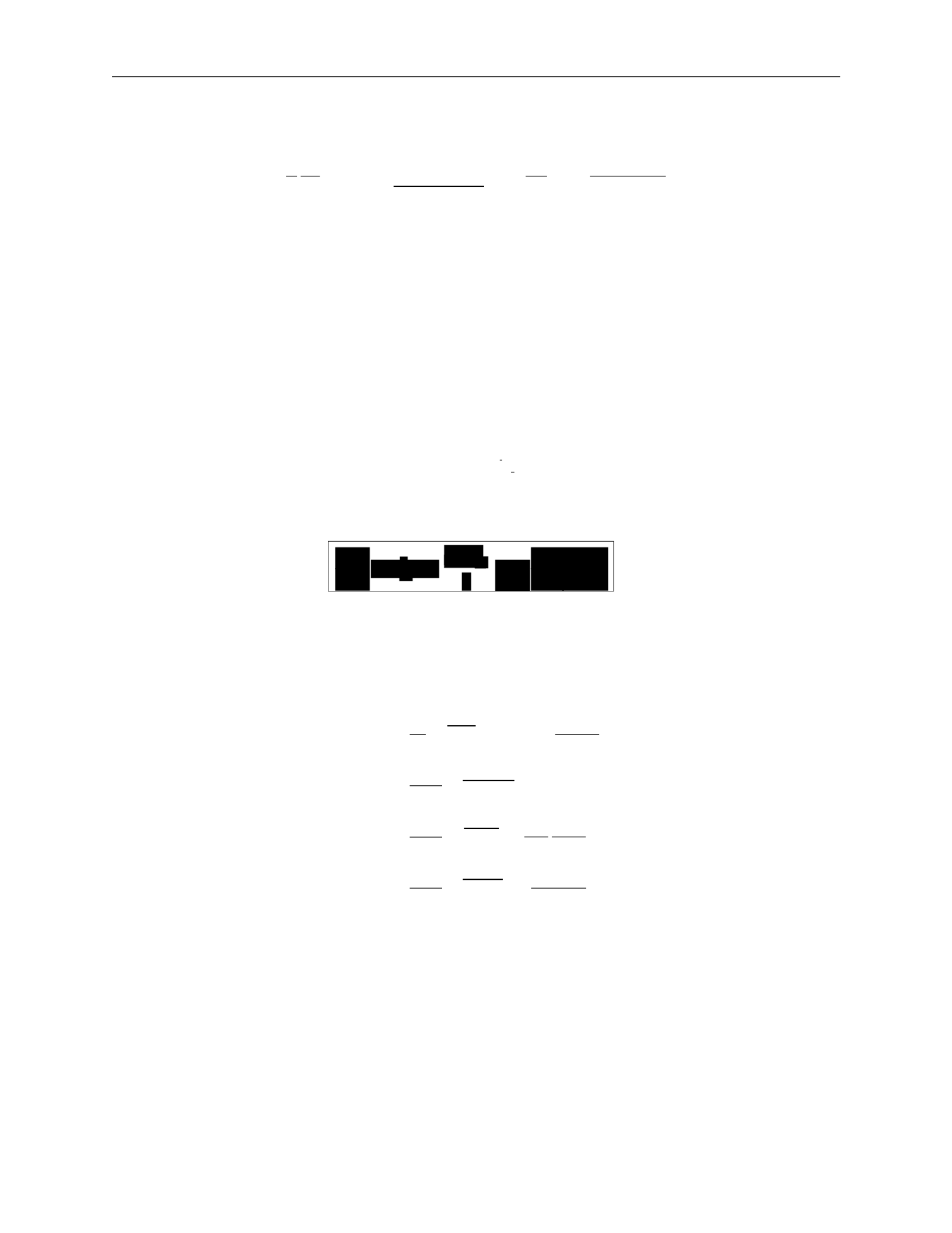
3.
MODELLING GALAXIES
43
2
2
2
2
t
t
t
— t
2
rr
rσ
rσ
rσ
rr
r
∂r
G
n
∂r
rr
—
dr
2
—
The simplified Jeans equation is:
1 ∂ 2(σ2
− σ ) ∂φ
GM (< r)
(nσ
2
) +
rr
t
=
−
=
−
(183)
where we’ve plugged in gravity as the force.
We have three limits we can look at:
•
σ
rr
•
σ
rr
•
σ
rr
σ
2
: nearly circular orbits
σ
2
: nearly radial orbits
= σ
2
: isotropic orbits
We define the anisotropy parameter:
σ
2
β
=
1
rr
(184)
which gives us a useful form of the Jeans equation for observations:
.
(185)
This depends only on radial components with uncertainty from
β
, assuming spherical sym-
metry and a steady-state system.
This can be simplified further to get mass estimates:
r2
1 ∂ 2 2βσ2
M (< r)
=
−
(nσ
)
+
2
=
−
rr
r
∂
(nσ
2
)
+
2β
G
2
=
rr
G
2
rr
r dn
+
n dr
rr
r
dσ
2
rr
+
2β
rr
(186)
2
=
rr
G
d ln n
+
d ln r
d ln σ2
rr
+
2β
d ln r
where the last line can be measured with observations.
Stability of stellar systems
The existence of equilibrium solutions to the collisionless Boltzmann equation does not assure stability.
Real stellar systems are subject to perturbations. What is important for stability?
1 ∂
2βσ2
σ
nσ
σ
n
∂r
r
2
r
∂r
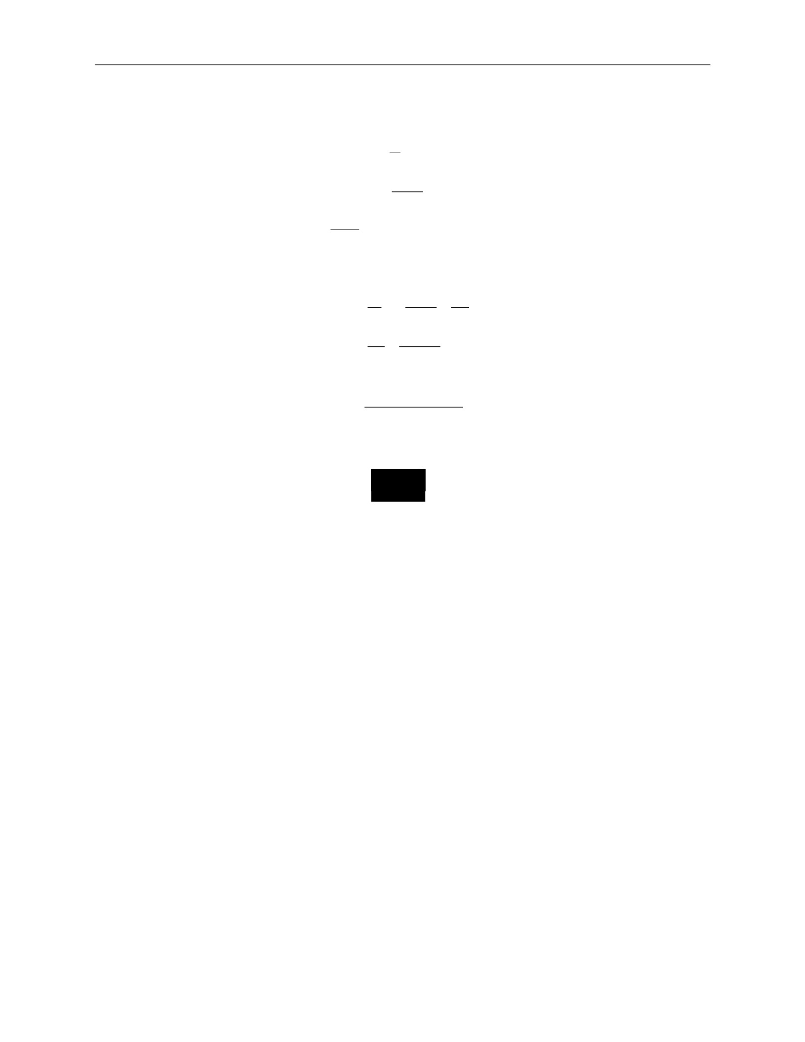
3.
MODELLING GALAXIES
38
v
·
Luminosity-velocity relations:
We can relate properties of a galaxy to observables through several equations:
R
θ
=
(apparent size)
d
L
F
=
4πd
2
(158)
v
2
=
GM .
R
Introducing surface brightness Σ
F
L
d
2
Σ =
=
θ
2
4πd
2
R
2
(159)
L
v
4
then
=
4π
·
G2M 2
v
4
L =
Σ4πG
2
(M/L)
2
.
(160)
If we assume, for a given class of galaxies, that the surface brightness and the mass-to-light
ratio are the same, then
.
(161)
This introduces two important relations.
The Tully-Fischer relation is used for spiral galaxies and relates the maximum velocity in
the rotation curve
v
max
, which can be measured from HII spectra, and the luminosity:
4
max
.
(162)
The Faber-Jackson relation is used for ellipticals and relates the velocity dispersion
σ
v
to the
luminosity:
L
∝
σ
4
.
(163)
Thus, we can get an estimate of the intrinsic luminosity of a galaxy be measuring stel-
lar velocities. The constant of proportionality is roughly
L
∗
/(220 km/s)
4
, where
L
∗
is the
characteristic galaxy luminosity.
3.P
Phase-space distribution function
We have described the individual orbits in a potential, but this is not sufficient to describe
galactic dynamics. We want information of the configuration of all particles. Each star is
described by its position
→
x
and velocity
→
v
,
and we need to know this for all stars, i.e. how
stars are distributed in the 6D phase space
(
→
x
,
→
v
)
.
We define a phase-space distribution function
f
(
→
x
,
→
v
,
t)d3
→
x
d
3
→
v
(164)
∝
L
∝
v
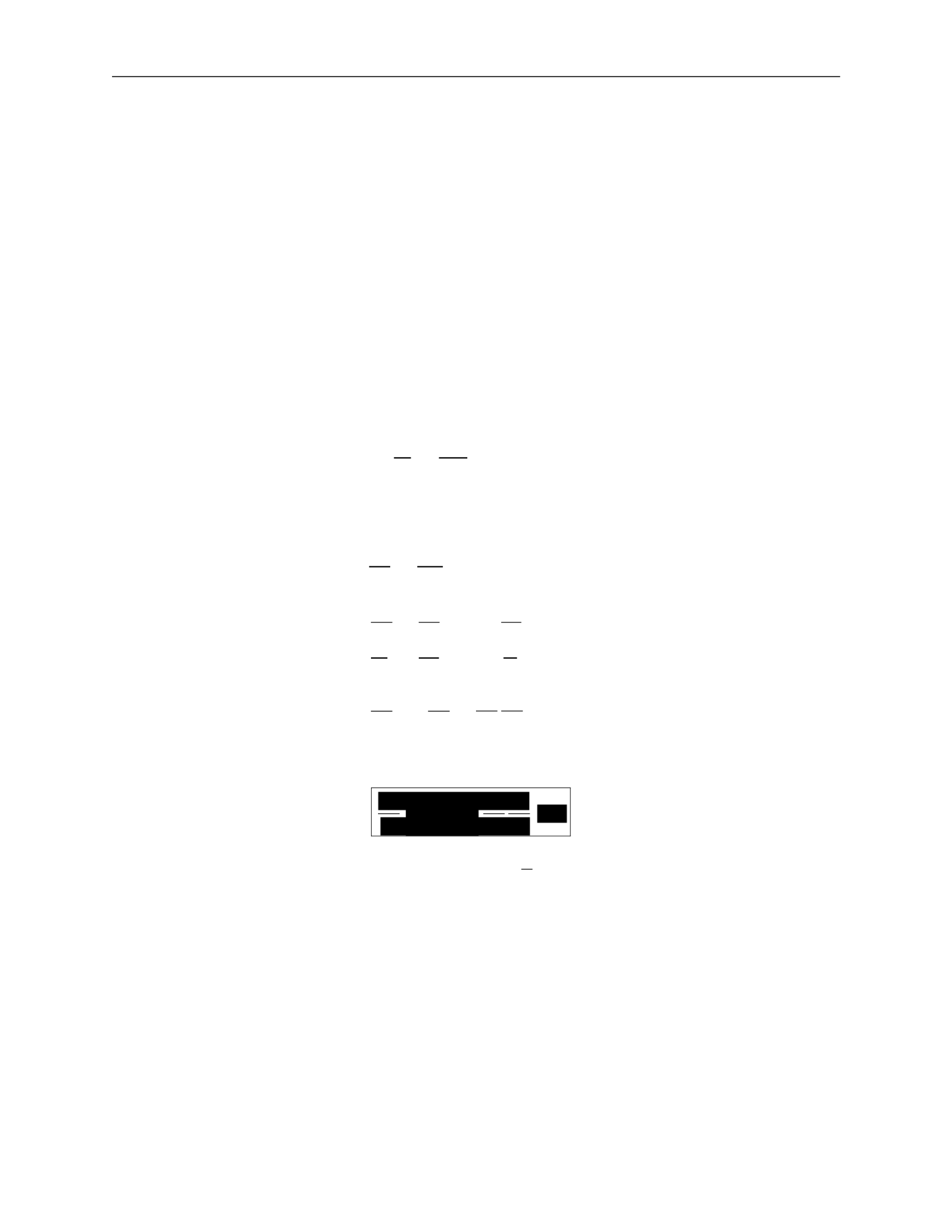
3.
MODELLING GALAXIES
39
∈
dt
as the probability that at time
t
, a randomly chosen star has
(
→
x
∗
,
→
v
∗
)
([
→
x
,
→
x
+
d
→
x
]
,
[
→
v
,
→
v
+
d
→
v])
.
This
means
that
the function must be normalized for all
t
, i.e.
∫
f
(
→
x
,
→
v
,
t)d
3
→
x
d
3
→
v
= 1 .
(165)
Collisionless
Boltzmann
equation
:
We want to describe the time evolution of
f
(
→
x
,
→
v
,
t)
. Since probability cannot be destroyed,
the 6D continuity equation must hold.
We define the 6D phase-space vector
then
w
→
=
(
→
x
,
→
v
)
(166)
∂f
+
∂
f
w
→
˙
=
0 .
(167)
∂t
∂w
→
This is the same form as the standard 3D continuity equation. We can rewrite this by
expanding out
w
→
and using velocity
→
v
=
→
x
˙
and acceleration
→
a
=
→
v
˙
:
0
= ∂f +
∂
f
w
→
˙
∂t
∂w
→
∂f
∂
=
+
∂t
∂
→
x
(
f
→
x
˙
) +
∂
(
f
→
v
˙
)
∂
→
v
(168)
∂f
∂
∂
=
+
(
f
→
v
)
+
f
(
−
∇
→
φ)
∂t
∂
→
x
∂
→
v
∂f
∂f
∂φ
∂f
=
∂t
+
→
v
∂
→
x
−
∂
→
x
∂
→
v
.
This gives us the collisionless Boltzmann equation (CBE):
.
(169)
Note that another way to see this is by writing out
df
= 0
and taking the limits
lim
→x
→∞
= 0
and
lim
→v
→∞
= 0
.
General Jeans equations:
A solution to the collisionless Boltzmann equation is difficult to obtain, so we instead study
moments of the CBE and the phase-space distribution.
Moments of the phase-space density give us some average quantities of the system.
a)
The first moment gives the density
n
of the system:
n
=
∫
f
d
3
→
v
.
(170)
∂t
−

3.
MODELLING GALAXIES
40
ij
∫
—
∫
∫
∫
±∞
—
i
n
i
i
j
n
i
j
∂
→
x
∂
→
v
∂
→
x
∂
→
v
∂
→
x
→v=
−∞
j
∂t
j
∂
→
x
j
∂
→
x
∂
→
v
2
b)
The second moment gives the average velocity
v
¯
i
:
v
¯
=
1
∫
v
f
d
3
→
v
.
(171)
c)
The third moment gives the velocity dispersion
σ
2
:
v v
=
1
∫
v v
f
d
3
→
v
ij
=
v
i
v
j
−
v
¯
i
v
¯
j
=
(v
i
−
v
¯
i
)(
v
j
−
v
¯
j
)
.
We now examine moments of the collisionless Boltzmann equation more closely. We break
each integral into three terms to simplify each individually.
aa)
First moment:
d
3
→
v
∂f
∂t
∂f
+
→
v
∂
→
x
∂φ
∂f
=
0
∂
→
x
∂
→
v
∫
d
3
→
v
∂f +
∫
d
3
→
v
→
v
∂f
−
∫
d
3
→
v
∂φ
∂f =
0 (173)
∂t
` ˛
1
¸ x
∂
→
x
` ˛
2
¸ x
∂
→
x
∂
→
v
` ˛
3
¸ x
:
d
3
→
v
∂f =
∂
∂t ∂t
d
3
→
v
f
=
∂n
∂t
:
d
3
→
v
→
v
∂f
∂
→
x
∂
=
∂
→
x
d3
→
v
→
v
f
=
∂
∂
→
x
n
→
v
¯
=
Σ
∂
∂x
i
(
n
v
¯
i
)
(174)
:
∫
d
3
→
v
∂φ
∂f
=
∂φ
∫
d
3
→
v
∂f
=
∂φ [f ]
→v=+
∞
=
0
For the third term, we used the fact that phase-space distribution goes to 0 at
for
physical systems.
This gives us the 3D continuity equation:
bb)
Second moment:
.
(175)
∫
d
3
→
v
vj
∂f
∂f
+
→
v
∂t
∂
→
x
∂φ
∂f
=
0
∂
→
x
∂
→
v
∫
d
3
→
v
v
∂f +
∫
d
3
→
v
v
→
v
∂f
−
∫
d
3
→
v
v
∂φ
∂f
=
0
(176)
` ˛
1
¸ x ` ˛
2
¸ x ` ˛
3
¸ x
1
2
3
∂n ∂
∂t
0
σ
∫
i
(172)

3.
MODELLING GALAXIES
41
ij
Σ
∫
i
∂x
∂x
j
∂t
∂t
j
∂t
j
∂t
∂t
∂x
i
∂t
∂t
j
∂x
i
using the continuity equation ∂n
=
−
Σ
∂
(
n
v
¯
)
j
∂
→
x
i
∂x
i
∂x
i
j
i
i
∂x
ij
i
j
∂x
j
∂v
j
v
i
=
−∞
i
∂v
∂t
∂x
i
∂x
ij
i
j
∂x
i
`
i
i
ij
i
∂x
i
∂v
:
∫
d
3
→
v
v
∂f =
∂
∫
d
3
→
v
v
f =
∂
(
n
v
¯
) =
∂
n
v
¯
+
n
∂
v
¯
j
=
−
v
¯
Σ
∂
(
n
v
¯
) +
n
∂
v
¯
j
=
n
∂
v
¯
j
−
v
¯
Σ
∂
(
n
v
¯
)
∂t
∂x
i
i
to go from the first line to the second
:
∫
d
3
→
v
v
→
v
∂f
=
∫
d
3
→
v
v
Σ
v
∂f =
Σ
∂
∫
d
3
→
v
v v
f
= nv
j
v
i
`
= n
˛ ¸
σ
2
+
x
v
¯
i
v
¯
j
=
Σ
∂
n
σ
2
+
v
¯
v
¯
:
∫
d
3
→
v
v
∂φ
∂f
=
∫
d
3
→
v
v
Σ
∂φ
∂f
=
Σ
∂φ
∫
d
3
→
v
v
∂f
(177)
((k, l, i) are permutations of (1, 2, 3))
=
∂φ
dv
∂x
k
∫
dv
l
∫
dv
i
∂f
v
j
∂v
=
[v
f
]
˛
v
¸
i
=+
∞
−
x
∫
dv ∂v
j
f
= 0
−
∫
dv
i
δ
ij
f
=
−
Σ
∂φ
∫
dv
∫
dv
l
∫
dv
i
δ
ij
f
i
i
=
−
Σ
∂φ
∫
d
3
→
v
δ
f
i
i
∂φ
=
−
n∂x
j
Plugging each term back in, we get
n
∂
v
¯
j
−
v
¯
Σ
∂
(
n
v
¯
) +
Σ
∂
n
σ
2
+
v
¯
v
¯
+
n
∂φ
=
0
(178)
i
i
i
i
i
i
i
i
i
i
i
1
2
3
j
j
i
j
i
i
j
∂
→
x
∂
→
v
j
i
i
i
j
k

3.
MODELLING GALAXIES
42
Σ
v
¯
2
2
∂t
j
∂x
i
∂x
ij
i
∂x
i
i
j
∂x
j
=
(
n
v
¯
i
)
∂
x
v
¯
j
+
v
¯
j
∂x
(
n
v
¯
i
)
∂t
i
∂x
j
∂x
ij
∂x
—
1
Σ
∂(nσ
ij
) :
pressure
∂t
i
i
i
i
i
i
i
i
j
which we can rewrite
n
∂
v
¯
j
−
v
¯
Σ
∂
(
n
v
¯
)
+
Σ
∂
(nσ
2
)+
Σ
∂
(
n
v
¯
v
¯
)
+n
∂φ
=
0
`
Σ˛¸
∂
x
Σ
∂
(179)
where the two underlined terms cancel. This gives us
n
∂
v
¯
j
+
Σ
(
n
v
¯
)
∂
v
¯
+
Σ
∂
(nσ
2
) +
n
∂φ
=
0 .
(180)
This is the Jeans equation, often written
(181)
Each term can be physically interpreted:
∂
v
¯
j
∂t
∂
v
¯
j
i
∂x
: acceleration of fluid
: kinematic viscosity/shear
i
i
2
(182)
n
∂x
i
∂φ
−
∂x
j
: gravity
Jeans
equations
in
spherical
systems
:
We can convert to spherical coordinates and take velocity moments to give us the Jeans
equations in spherical coordinates. This is complicated!
To simplify, we take the radial Jeans equation and focus on steady-state symmetric systems.
Implications:
∂
=
0
since we have steady state
•
v
¯
r
=
0
otherwise we have net radial motion
•
v
¯
θ
=
v
¯
φ
=
0
or the symmetry is broken
•
σ
rφ
=
0
or the symmetry is broken
2
•
σ
φφ
≡
σ
or the symmetry is broken.
2
2
rθ
θθ
t
∂φ
1
∂t
•
=
σ
=
σ
i
i
i
i
i

3.
MODELLING GALAXIES
43
2
2
2
2
t
t
t
— t
2
rr
rσ
rσ
rσ
rr
r
∂r
G
n
∂r
rr
—
dr
2
—
The simplified Jeans equation is:
1 ∂ 2(σ2
− σ ) ∂φ
GM (< r)
(nσ
2
) +
rr
t
=
−
=
−
(183)
where we’ve plugged in gravity as the force.
We have three limits we can look at:
•
σ
rr
•
σ
rr
•
σ
rr
σ
2
: nearly circular orbits
σ
2
: nearly radial orbits
= σ
2
: isotropic orbits
We define the anisotropy parameter:
σ
2
β
=
1
rr
(184)
which gives us a useful form of the Jeans equation for observations:
.
(185)
This depends only on radial components with uncertainty from
β
, assuming spherical sym-
metry and a steady-state system.
This can be simplified further to get mass estimates:
r2
1 ∂ 2 2βσ2
M (< r)
=
−
(nσ
)
+
2
=
−
rr
r
∂
(nσ
2
)
+
2β
G
2
=
rr
G
2
rr
r dn
+
n dr
rr
r
dσ
2
rr
+
2β
rr
(186)
2
=
rr
G
d ln n
+
d ln r
d ln σ2
rr
+
2β
d ln r
where the last line can be measured with observations.
Stability of stellar systems
The existence of equilibrium solutions to the collisionless Boltzmann equation does not assure
stability. Real stellar systems are subject to perturbations. What is important for stability?
1 ∂
2βσ2
σ
nσ
σ
n
∂r
r
2
r
∂r
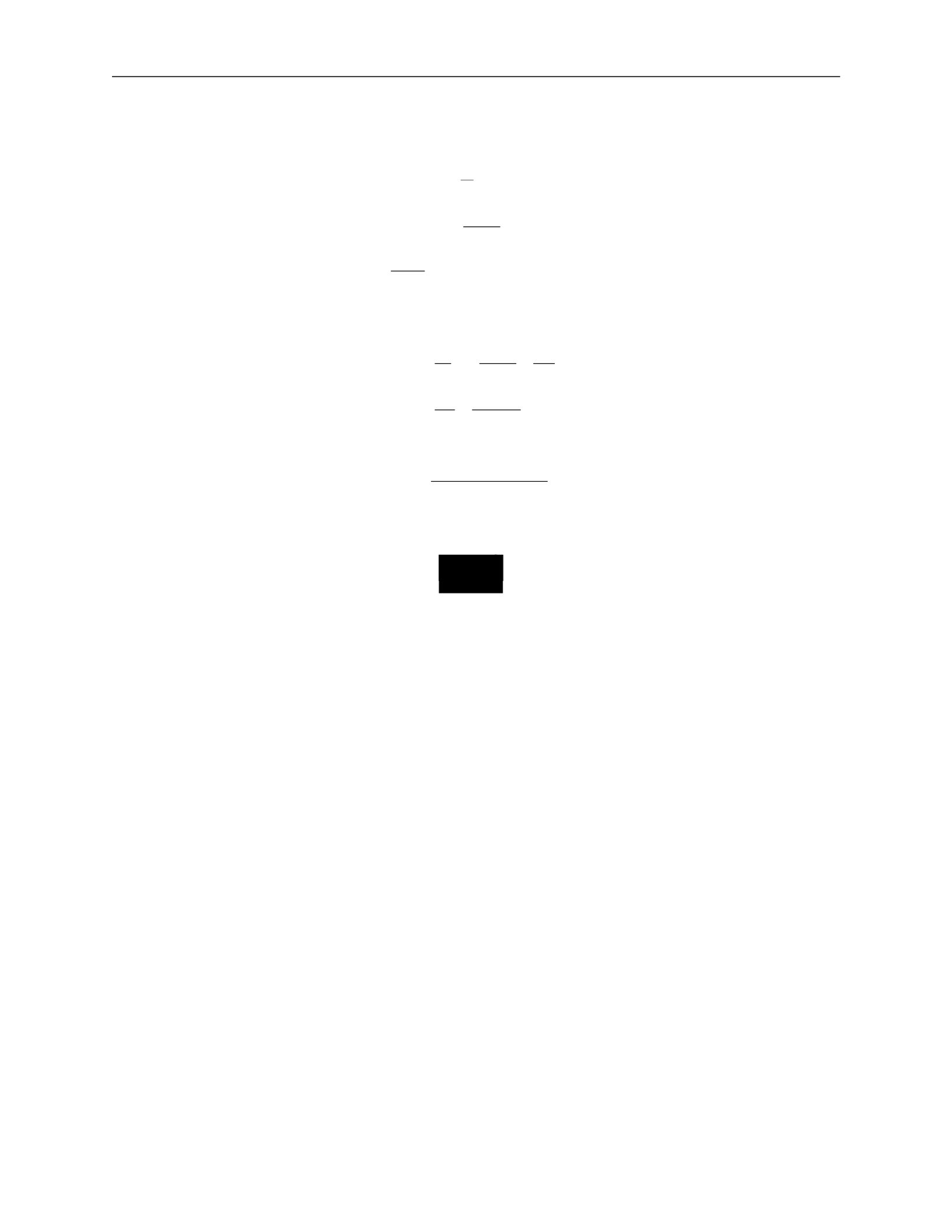
3.
MODELLING GALAXIES
38
v
·
Luminosity-velocity relations:
We can relate properties of a galaxy to observables through several equations:
R
θ
=
(apparent size)
d
L
F
=
4πd
2
(158)
v
2
=
GM .
R
Introducing surface brightness Σ
F
L
d
2
Σ =
=
θ
2
4πd
2
R
2
(159)
L
v
4
then
=
4π
·
G2M 2
v
4
L =
Σ4πG
2
(M/L)
2
.
(160)
If we assume, for a given class of galaxies, that the surface brightness and the mass-to-light
ratio are the same, then
.
(161)
This introduces two important relations.
The Tully-Fischer relation is used for spiral galaxies and relates the maximum velocity in
the rotation curve
v
max
, which can be measured from HII spectra, and the luminosity:
4
max
.
(162)
The Faber-Jackson relation is used for ellipticals and relates the velocity dispersion
σ
v
to the
luminosity:
L
∝
σ
4
.
(163)
Thus, we can get an estimate of the intrinsic luminosity of a galaxy be measuring stel-
lar velocities. The constant of proportionality is roughly
L
∗
/(220 km/s)
4
, where
L
∗
is the
characteristic galaxy luminosity.
3.Q
Phase-space distribution function
We have described the individual orbits in a potential, but this is not sufficient to describe
galactic dynamics. We want information of the configuration of all particles. Each star is
described by its position
→
x
and velocity
→
v
,
and we need to know this for all stars, i.e. how
stars are distributed in the 6D phase space
(
→
x
,
→
v
)
.
We define a phase-space distribution function
f
(
→
x
,
→
v
,
t)d3
→
x
d
3
→
v
(164)
∝
L
∝
v
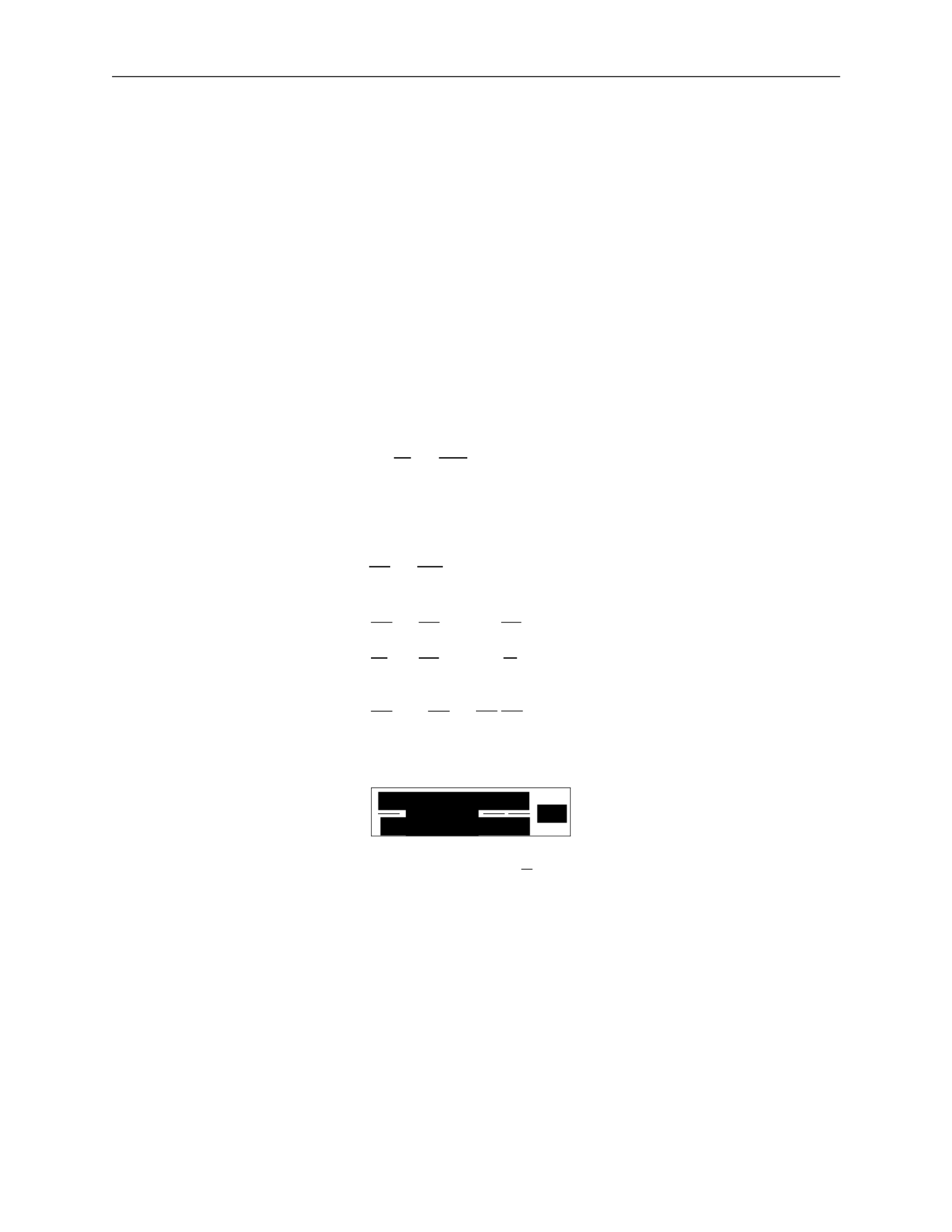
3.
MODELLING GALAXIES
39
∈
dt
as the probability that at time
t
, a randomly chosen star has
(
→
x
∗
,
→
v
∗
)
([
→
x
,
→
x
+
d
→
x
]
,
[
→
v
,
→
v
+
d
→
v])
.
This
means
that
the function must be normalized for all
t
, i.e.
∫
f
(
→
x
,
→
v
,
t)d
3
→
x
d
3
→
v
= 1 .
(165)
Collisionless
Boltzmann
equation
:
We want to describe the time evolution of
f
(
→
x
,
→
v
,
t)
. Since probability cannot be destroyed,
the 6D continuity equation must hold.
We define the 6D phase-space vector
then
w
→
=
(
→
x
,
→
v
)
(166)
∂f
+
∂
f
w
→
˙
=
0 .
(167)
∂t
∂w
→
This is the same form as the standard 3D continuity equation. We can rewrite this by
expanding out
w
→
and using velocity
→
v
=
→
x
˙
and acceleration
→
a
=
→
v
˙
:
0
= ∂f +
∂
f
w
→
˙
∂t
∂w
→
∂f
∂
=
+
∂t
∂
→
x
(
f
→
x
˙
) +
∂
(
f
→
v
˙
)
∂
→
v
(168)
∂f
∂
∂
=
+
(
f
→
v
)
+
f
(
−
∇
→
φ)
∂t
∂
→
x
∂
→
v
∂f
∂f
∂φ
∂f
=
∂t
+
→
v
∂
→
x
−
∂
→
x
∂
→
v
.
This gives us the collisionless Boltzmann equation (CBE):
.
(169)
Note that another way to see this is by writing out
df
= 0
and taking the limits
lim
→x
→∞
= 0
and
lim
→v
→∞
= 0
.
General Jeans equations:
A solution to the collisionless Boltzmann equation is difficult to obtain, so we instead study
moments of the CBE and the phase-space distribution.
Moments of the phase-space density give us some average quantities of the system.
a)
The first moment gives the density
n
of the system:
n
=
∫
f
d
3
→
v
.
(170)
∂t
−
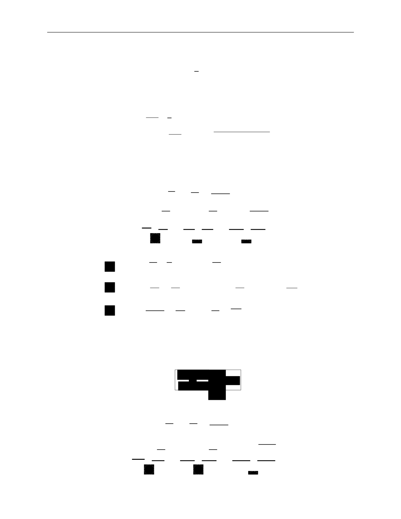
3.
MODELLING GALAXIES
40
ij
∫
—
∫
∫
∫
±∞
—
i
n
i
i
j
n
i
j
∂
→
x
∂
→
v
∂
→
x
∂
→
v
∂
→
x
→v=
−∞
j
∂t
j
∂
→
x
j
∂
→
x
∂
→
v
2
b)
The second moment gives the average velocity
v
¯
i
:
v
¯
=
1
∫
v
f
d
3
→
v
.
(171)
c)
The third moment gives the velocity dispersion
σ
2
:
v v
=
1
∫
v v
f
d
3
→
v
ij
=
v
i
v
j
−
v
¯
i
v
¯
j
=
(v
i
−
v
¯
i
)(
v
j
−
v
¯
j
)
.
We now examine moments of the collisionless Boltzmann equation more closely. We break
each integral into three terms to simplify each individually.
cc)
First moment:
d
3
→
v
∂f
∂t
∂f
+
→
v
∂
→
x
∂φ
∂f
=
0
∂
→
x
∂
→
v
∫
d
3
→
v
∂f +
∫
d
3
→
v
→
v
∂f
−
∫
d
3
→
v
∂φ
∂f =
0 (173)
∂t
` ˛
1
¸ x
∂
→
x
` ˛
2
¸ x
∂
→
x
∂
→
v
` ˛
3
¸ x
:
d
3
→
v
∂f =
∂
∂t ∂t
d
3
→
v
f
=
∂n
∂t
:
d
3
→
v
→
v
∂f
∂
→
x
∂
=
∂
→
x
d3
→
v
→
v
f
=
∂
∂
→
x
n
→
v
¯
=
Σ
∂
∂x
i
(
n
v
¯
i
)
(174)
:
∫
d
3
→
v
∂φ
∂f
=
∂φ
∫
d
3
→
v
∂f
=
∂φ [f ]
→v=+
∞
=
0
For the third term, we used the fact that phase-space distribution goes to 0 at
for
physical systems.
This gives us the 3D continuity equation:
dd)
Second moment:
.
(175)
∫
d
3
→
v
vj
∂f
∂f
+
→
v
∂t
∂
→
x
∂φ
∂f
=
0
∂
→
x
∂
→
v
∫
d
3
→
v
v
∂f +
∫
d
3
→
v
v
→
v
∂f
−
∫
d
3
→
v
v
∂φ
∂f
=
0
(176)
` ˛
1
¸ x ` ˛
2
¸ x ` ˛
3
¸ x
1
2
3
∂n ∂
∂t
0
σ
∫
i
(172)

3.
MODELLING GALAXIES
41
ij
Σ
∫
i
∂x
∂x
j
∂t
∂t
j
∂t
j
∂t
∂t
∂x
i
∂t
∂t
j
∂x
i
using the continuity equation ∂n
=
−
Σ
∂
(
n
v
¯
)
j
∂
→
x
i
∂x
i
∂x
i
j
i
i
∂x
ij
i
j
∂x
j
∂v
j
v
i
=
−∞
i
∂v
∂t
∂x
i
∂x
ij
i
j
∂x
i
`
i
i
ij
i
∂x
i
∂v
:
∫
d
3
→
v
v
∂f =
∂
∫
d
3
→
v
v
f =
∂
(
n
v
¯
) =
∂
n
v
¯
+
n
∂
v
¯
j
=
−
v
¯
Σ
∂
(
n
v
¯
) +
n
∂
v
¯
j
=
n
∂
v
¯
j
−
v
¯
Σ
∂
(
n
v
¯
)
∂t
∂x
i
i
to go from the first line to the second
:
∫
d
3
→
v
v
→
v
∂f
=
∫
d
3
→
v
v
Σ
v
∂f =
Σ
∂
∫
d
3
→
v
v v
f
= nv
j
v
i
`
= n
˛ ¸
σ
2
+
x
v
¯
i
v
¯
j
=
Σ
∂
n
σ
2
+
v
¯
v
¯
:
∫
d
3
→
v
v
∂φ
∂f
=
∫
d
3
→
v
v
Σ
∂φ
∂f
=
Σ
∂φ
∫
d
3
→
v
v
∂f
(177)
((k, l, i) are permutations of (1, 2, 3))
=
∂φ
dv
∂x
k
∫
dv
l
∫
dv
i
∂f
v
j
∂v
=
[v
f
]
˛
v
¸
i
=+
∞
−
x
∫
dv ∂v
j
f
= 0
−
∫
dv
i
δ
ij
f
=
−
Σ
∂φ
∫
dv
∫
dv
l
∫
dv
i
δ
ij
f
i
i
=
−
Σ
∂φ
∫
d
3
→
v
δ
f
i
i
∂φ
=
−
n∂x
j
Plugging each term back in, we get
n
∂
v
¯
j
−
v
¯
Σ
∂
(
n
v
¯
) +
Σ
∂
n
σ
2
+
v
¯
v
¯
+
n
∂φ
=
0
(178)
i
i
i
i
i
i
i
i
i
i
i
1
2
3
j
j
i
j
i
i
j
∂
→
x
∂
→
v
j
i
i
i
j
k

3.
MODELLING GALAXIES
42
Σ
v
¯
2
2
∂t
j
∂x
i
∂x
ij
i
∂x
i
i
j
∂x
j
=
(
n
v
¯
i
)
∂
x
v
¯
j
+
v
¯
j
∂x
(
n
v
¯
i
)
∂t
i
∂x
j
∂x
ij
∂x
—
1
Σ
∂(nσ
ij
) :
pressure
∂t
i
i
i
i
i
i
i
i
j
which we can rewrite
n
∂
v
¯
j
−
v
¯
Σ
∂
(
n
v
¯
)
+
Σ
∂
(nσ
2
)+
Σ
∂
(
n
v
¯
v
¯
)
+n
∂φ
=
0
`
Σ˛¸
∂
x
Σ
∂
(179)
where the two underlined terms cancel. This gives us
n
∂
v
¯
j
+
Σ
(
n
v
¯
)
∂
v
¯
+
Σ
∂
(nσ
2
) +
n
∂φ
=
0 .
(180)
This is the Jeans equation, often written
(181)
Each term can be physically interpreted:
∂
v
¯
j
∂t
∂
v
¯
j
i
∂x
: acceleration of fluid
: kinematic viscosity/shear
i
i
2
(182)
n
∂x
i
∂φ
−
∂x
j
: gravity
Jeans
equations
in
spherical
systems
:
We can convert to spherical coordinates and take velocity moments to give us the Jeans
equations in spherical coordinates. This is complicated!
To simplify, we take the radial Jeans equation and focus on steady-state symmetric systems.
Implications:
∂
=
0
since we have steady state
•
v
¯
r
=
0
otherwise we have net radial motion
•
v
¯
θ
=
v
¯
φ
=
0
or the symmetry is broken
•
σ
rφ
=
0
or the symmetry is broken
2
•
σ
φφ
≡
σ
or the symmetry is broken.
2
2
rθ
θθ
t
∂φ
1
∂t
•
=
σ
=
σ
i
i
i
i
i
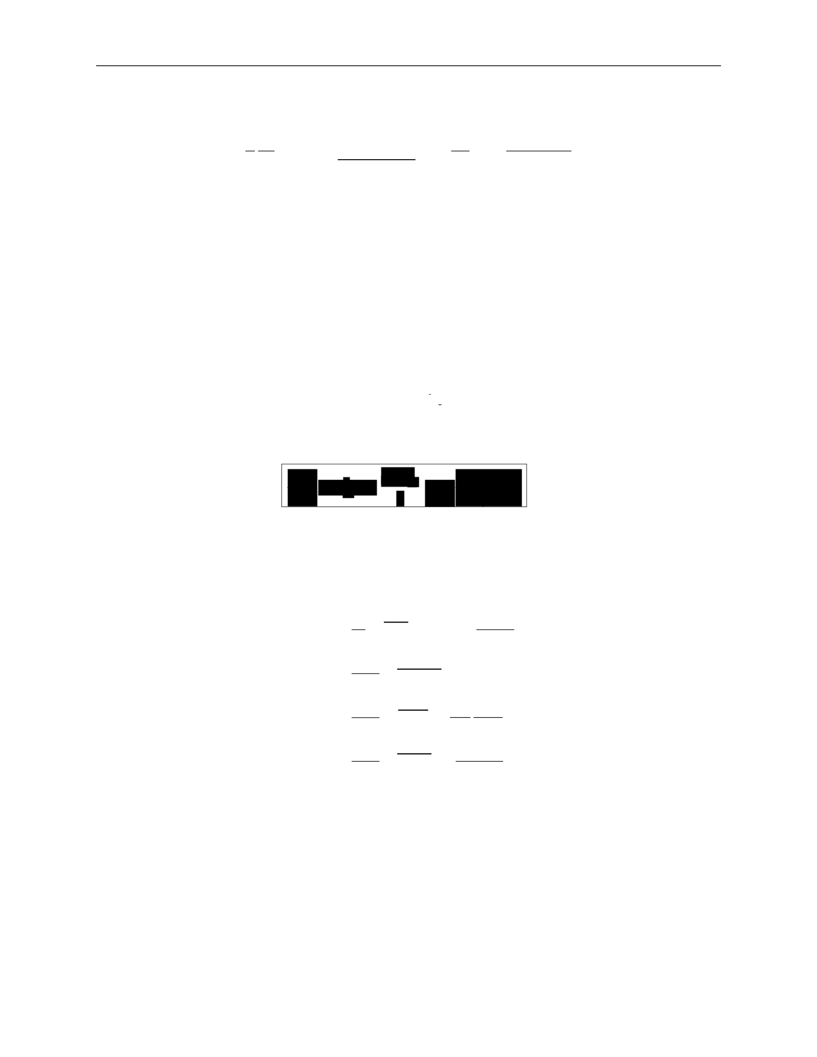
3.
MODELLING GALAXIES
43
2
2
2
2
t
t
t
— t
2
rr
rσ
rσ
rσ
rr
r
∂r
G
n
∂r
rr
—
dr
2
—
The simplified Jeans equation is:
1 ∂ 2(σ2
− σ ) ∂φ
GM (< r)
(nσ
2
) +
rr
t
=
−
=
−
(183)
where we’ve plugged in gravity as the force.
We have three limits we can look at:
•
σ
rr
•
σ
rr
•
σ
rr
σ
2
: nearly circular orbits
σ
2
: nearly radial orbits
= σ
2
: isotropic orbits
We define the anisotropy parameter:
σ
2
β
=
1
rr
(184)
which gives us a useful form of the Jeans equation for observations:
.
(185)
This depends only on radial components with uncertainty from
β
, assuming spherical sym-
metry and a steady-state system.
This can be simplified further to get mass estimates:
r2
1 ∂ 2 2βσ2
M (< r)
=
−
(nσ
)
+
2
=
−
rr
r
∂
(nσ
2
)
+
2β
G
2
=
rr
G
2
rr
r dn
+
n dr
rr
r
dσ
2
rr
+
2β
rr
(186)
2
=
rr
G
d ln n
+
d ln r
d ln σ2
rr
+
2β
d ln r
where the last line can be measured with observations.
Stability of stellar systems
The existence of equilibrium solutions to the collisionless Boltzmann equation does not assure stability.
Real stellar systems are subject to perturbations. What is important for stability?
1 ∂
2βσ2
σ
nσ
σ
n
∂r
r
2
r
∂r
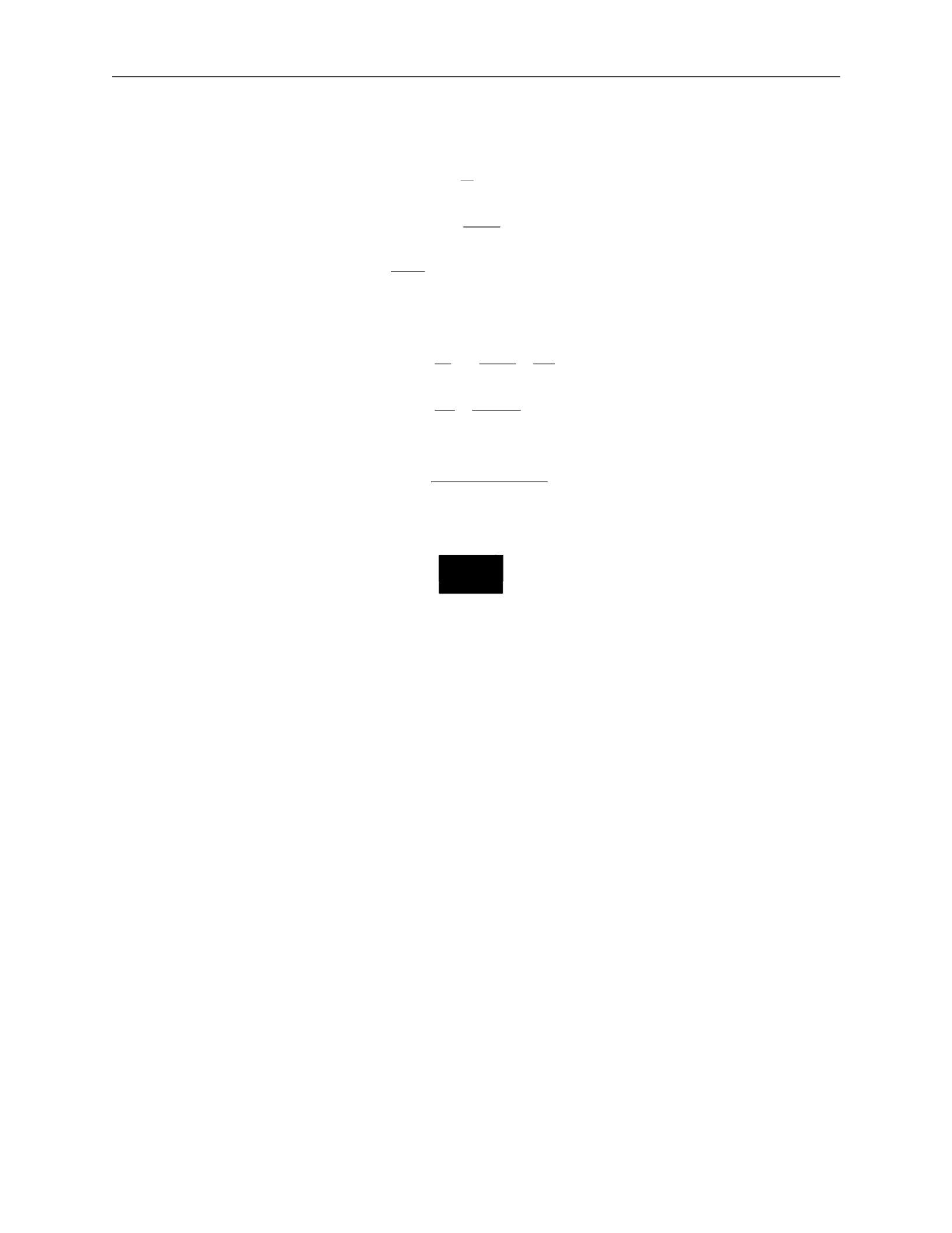
3.
MODELLING GALAXIES
38
v
·
Luminosity-velocity relations:
We can relate properties of a galaxy to observables through several equations:
R
θ
=
(apparent size)
d
L
F
=
4πd
2
(158)
v
2
=
GM .
R
Introducing surface brightness Σ
F
L
d
2
Σ =
=
θ
2
4πd
2
R
2
(159)
L
v
4
then
=
4π
·
G2M 2
v
4
L =
Σ4πG
2
(M/L)
2
.
(160)
If we assume, for a given class of galaxies, that the surface brightness and the mass-to-light
ratio are the same, then
.
(161)
This introduces two important relations.
The Tully-Fischer relation is used for spiral galaxies and relates the maximum velocity in
the rotation curve
v
max
, which can be measured from HII spectra, and the luminosity:
4
max
.
(162)
The Faber-Jackson relation is used for ellipticals and relates the velocity dispersion
σ
v
to the
luminosity:
L
∝
σ
4
.
(163)
Thus, we can get an estimate of the intrinsic luminosity of a galaxy be measuring stel-
lar velocities. The constant of proportionality is roughly
L
∗
/(220 km/s)
4
, where
L
∗
is the
characteristic galaxy luminosity.
3.R
Phase-space distribution function
We have described the individual orbits in a potential, but this is not sufficient to describe
galactic dynamics. We want information of the configuration of all particles. Each star is
described by its position
→
x
and velocity
→
v
,
and we need to know this for all stars, i.e. how
stars are distributed in the 6D phase space
(
→
x
,
→
v
)
.
We define a phase-space distribution function
f
(
→
x
,
→
v
,
t)d3
→
x
d
3
→
v
(164)
∝
L
∝
v
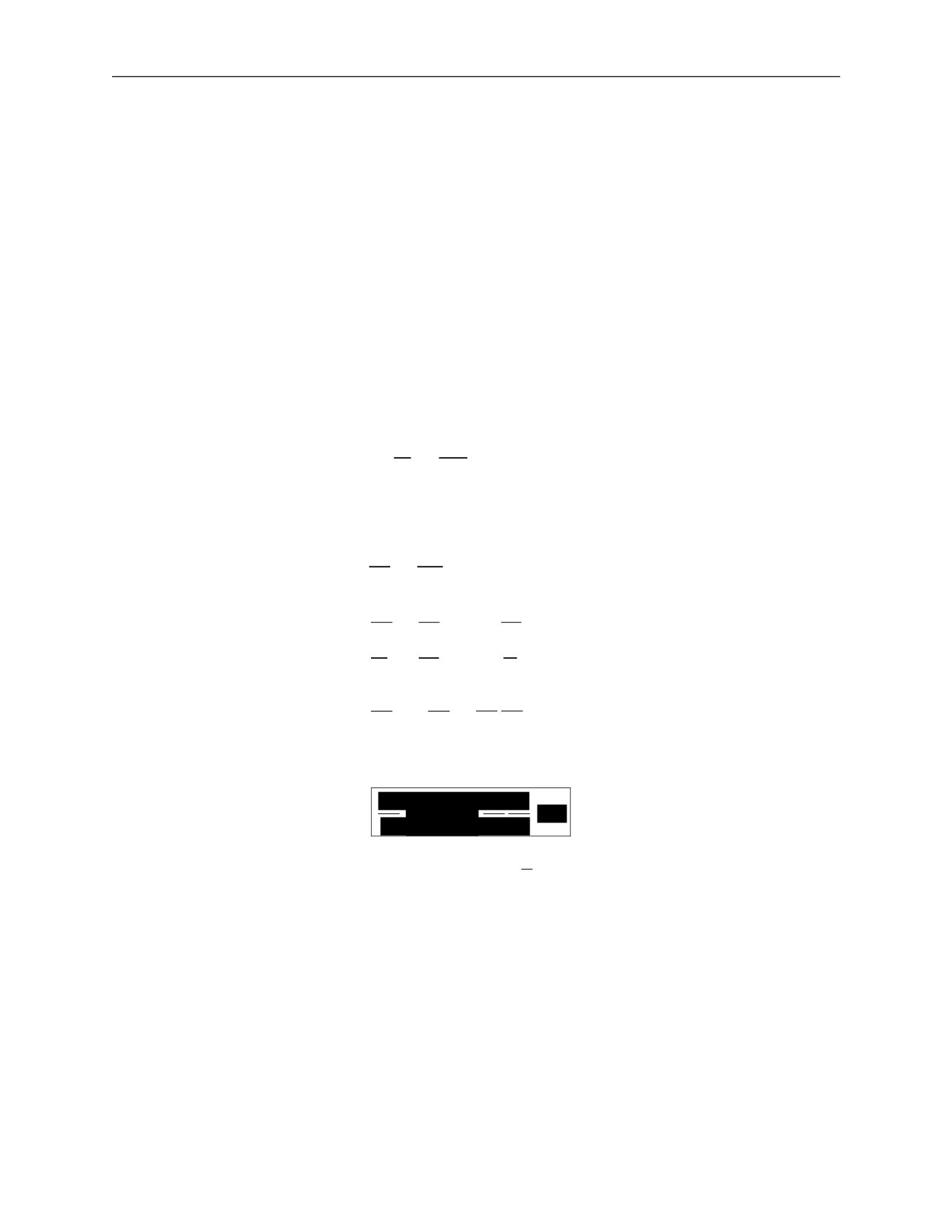
3.
MODELLING GALAXIES
39
∈
dt
as the probability that at time
t
, a randomly chosen star has
(
→
x
∗
,
→
v
∗
)
([
→
x
,
→
x
+
d
→
x
]
,
[
→
v
,
→
v
+
d
→
v])
.
This
means
that
the function must be normalized for all
t
, i.e.
∫
f
(
→
x
,
→
v
,
t)d
3
→
x
d
3
→
v
= 1 .
(165)
Collisionless
Boltzmann
equation
:
We want to describe the time evolution of
f
(
→
x
,
→
v
,
t)
. Since probability cannot be destroyed,
the 6D continuity equation must hold.
We define the 6D phase-space vector
then
w
→
=
(
→
x
,
→
v
)
(166)
∂f
+
∂
f
w
→
˙
=
0 .
(167)
∂t
∂w
→
This is the same form as the standard 3D continuity equation. We can rewrite this by
expanding out
w
→
and using velocity
→
v
=
→
x
˙
and acceleration
→
a
=
→
v
˙
:
0
= ∂f +
∂
f
w
→
˙
∂t
∂w
→
∂f
∂
=
+
∂t
∂
→
x
(
f
→
x
˙
) +
∂
(
f
→
v
˙
)
∂
→
v
(168)
∂f
∂
∂
=
+
(
f
→
v
)
+
f
(
−
∇
→
φ)
∂t
∂
→
x
∂
→
v
∂f
∂f
∂φ
∂f
=
∂t
+
→
v
∂
→
x
−
∂
→
x
∂
→
v
.
This gives us the collisionless Boltzmann equation (CBE):
.
(169)
Note that another way to see this is by writing out
df
= 0
and taking the limits
lim
→x
→∞
= 0
and
lim
→v
→∞
= 0
.
General Jeans equations:
A solution to the collisionless Boltzmann equation is difficult to obtain, so we instead study
moments of the CBE and the phase-space distribution.
Moments of the phase-space density give us some average quantities of the system.
a)
The first moment gives the density
n
of the system:
n
=
∫
f
d
3
→
v
.
(170)
∂t
−
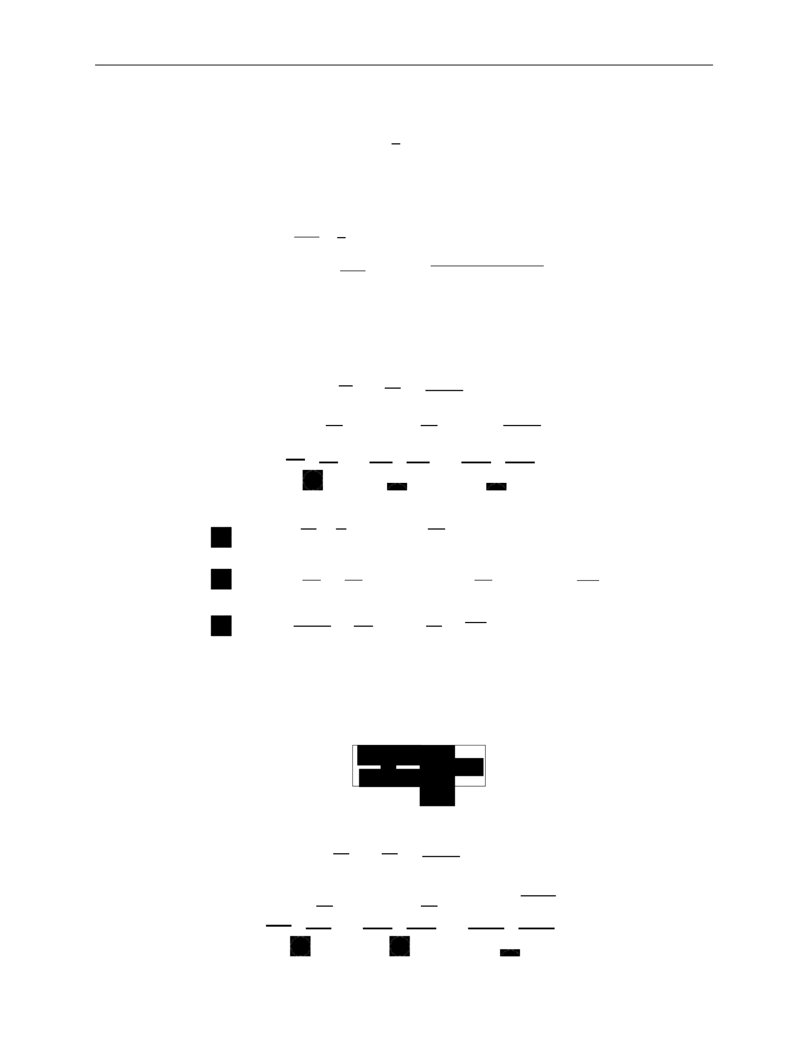
3.
MODELLING GALAXIES
40
ij
∫
—
∫
∫
∫
±∞
—
i
n
i
i
j
n
i
j
∂
→
x
∂
→
v
∂
→
x
∂
→
v
∂
→
x
→v=
−∞
j
∂t
j
∂
→
x
j
∂
→
x
∂
→
v
2
b)
The second moment gives the average velocity
v
¯
i
:
v
¯
=
1
∫
v
f
d
3
→
v
.
(171)
c)
The third moment gives the velocity dispersion
σ
2
:
v v
=
1
∫
v v
f
d
3
→
v
ij
=
v
i
v
j
−
v
¯
i
v
¯
j
=
(v
i
−
v
¯
i
)(
v
j
−
v
¯
j
)
.
We now examine moments of the collisionless Boltzmann equation more closely. We break
each integral into three terms to simplify each individually.
ee)
First moment:
d
3
→
v
∂f
∂t
∂f
+
→
v
∂
→
x
∂φ
∂f
=
0
∂
→
x
∂
→
v
∫
d
3
→
v
∂f +
∫
d
3
→
v
→
v
∂f
−
∫
d
3
→
v
∂φ
∂f =
0 (173)
∂t
` ˛
1
¸ x
∂
→
x
` ˛
2
¸ x
∂
→
x
∂
→
v
` ˛
3
¸ x
:
d
3
→
v
∂f =
∂
∂t ∂t
d
3
→
v
f
=
∂n
∂t
:
d
3
→
v
→
v
∂f
∂
→
x
∂
=
∂
→
x
d3
→
v
→
v
f
=
∂
∂
→
x
n
→
v
¯
=
Σ
∂
∂x
i
(
n
v
¯
i
)
(174)
:
∫
d
3
→
v
∂φ
∂f
=
∂φ
∫
d
3
→
v
∂f
=
∂φ [f ]
→v=+
∞
=
0
For the third term, we used the fact that phase-space distribution goes to 0 at
for
physical systems.
This gives us the 3D continuity equation:
ff)
Second moment:
.
(175)
∫
d
3
→
v
vj
∂f
∂f
+
→
v
∂t
∂
→
x
∂φ
∂f
=
0
∂
→
x
∂
→
v
∫
d
3
→
v
v
∂f +
∫
d
3
→
v
v
→
v
∂f
−
∫
d
3
→
v
v
∂φ
∂f
=
0
(176)
` ˛
1
¸ x ` ˛
2
¸ x ` ˛
3
¸ x
1
2
3
∂n ∂
∂t
0
σ
∫
i
(172)

3.
MODELLING GALAXIES
41
ij
Σ
∫
i
∂x
∂x
j
∂t
∂t
j
∂t
j
∂t
∂t
∂x
i
∂t
∂t
j
∂x
i
using the continuity equation ∂n
=
−
Σ
∂
(
n
v
¯
)
j
∂
→
x
i
∂x
i
∂x
i
j
i
i
∂x
ij
i
j
∂x
j
∂v
j
v
i
=
−∞
i
∂v
∂t
∂x
i
∂x
ij
i
j
∂x
i
`
i
i
ij
i
∂x
i
∂v
:
∫
d
3
→
v
v
∂f =
∂
∫
d
3
→
v
v
f =
∂
(
n
v
¯
) =
∂
n
v
¯
+
n
∂
v
¯
j
=
−
v
¯
Σ
∂
(
n
v
¯
) +
n
∂
v
¯
j
=
n
∂
v
¯
j
−
v
¯
Σ
∂
(
n
v
¯
)
∂t
∂x
i
i
to go from the first line to the second
:
∫
d
3
→
v
v
→
v
∂f
=
∫
d
3
→
v
v
Σ
v
∂f =
Σ
∂
∫
d
3
→
v
v v
f
= nv
j
v
i
`
= n
˛ ¸
σ
2
+
x
v
¯
i
v
¯
j
=
Σ
∂
n
σ
2
+
v
¯
v
¯
:
∫
d
3
→
v
v
∂φ
∂f
=
∫
d
3
→
v
v
Σ
∂φ
∂f
=
Σ
∂φ
∫
d
3
→
v
v
∂f
(177)
((k, l, i) are permutations of (1, 2, 3))
=
∂φ
dv
∂x
k
∫
dv
l
∫
dv
i
∂f
v
j
∂v
=
[v
f
]
˛
v
¸
i
=+
∞
−
x
∫
dv ∂v
j
f
= 0
−
∫
dv
i
δ
ij
f
=
−
Σ
∂φ
∫
dv
∫
dv
l
∫
dv
i
δ
ij
f
i
i
=
−
Σ
∂φ
∫
d
3
→
v
δ
f
i
i
∂φ
=
−
n∂x
j
Plugging each term back in, we get
n
∂
v
¯
j
−
v
¯
Σ
∂
(
n
v
¯
) +
Σ
∂
n
σ
2
+
v
¯
v
¯
+
n
∂φ
=
0
(178)
i
i
i
i
i
i
i
i
i
i
i
1
2
3
j
j
i
j
i
i
j
∂
→
x
∂
→
v
j
i
i
i
j
k

3.
MODELLING GALAXIES
42
Σ
v
¯
2
2
∂t
j
∂x
i
∂x
ij
i
∂x
i
i
j
∂x
j
=
(
n
v
¯
i
)
∂
x
v
¯
j
+
v
¯
j
∂x
(
n
v
¯
i
)
∂t
i
∂x
j
∂x
ij
∂x
—
1
Σ
∂(nσ
ij
) :
pressure
∂t
i
i
i
i
i
i
i
i
j
which we can rewrite
n
∂
v
¯
j
−
v
¯
Σ
∂
(
n
v
¯
)
+
Σ
∂
(nσ
2
)+
Σ
∂
(
n
v
¯
v
¯
)
+n
∂φ
=
0
`
Σ˛¸
∂
x
Σ
∂
(179)
where the two underlined terms cancel. This gives us
n
∂
v
¯
j
+
Σ
(
n
v
¯
)
∂
v
¯
+
Σ
∂
(nσ
2
) +
n
∂φ
=
0 .
(180)
This is the Jeans equation, often written
(181)
Each term can be physically interpreted:
∂
v
¯
j
∂t
∂
v
¯
j
i
∂x
: acceleration of fluid
: kinematic viscosity/shear
i
i
2
(182)
n
∂x
i
∂φ
−
∂x
j
: gravity
Jeans
equations
in
spherical
systems
:
We can convert to spherical coordinates and take velocity moments to give us the Jeans
equations in spherical coordinates. This is complicated!
To simplify, we take the radial Jeans equation and focus on steady-state symmetric systems.
Implications:
∂
=
0
since we have steady state
•
v
¯
r
=
0
otherwise we have net radial motion
•
v
¯
θ
=
v
¯
φ
=
0
or the symmetry is broken
•
σ
rφ
=
0
or the symmetry is broken
2
•
σ
φφ
≡
σ
or the symmetry is broken.
2
2
rθ
θθ
t
∂φ
1
∂t
•
=
σ
=
σ
i
i
i
i
i
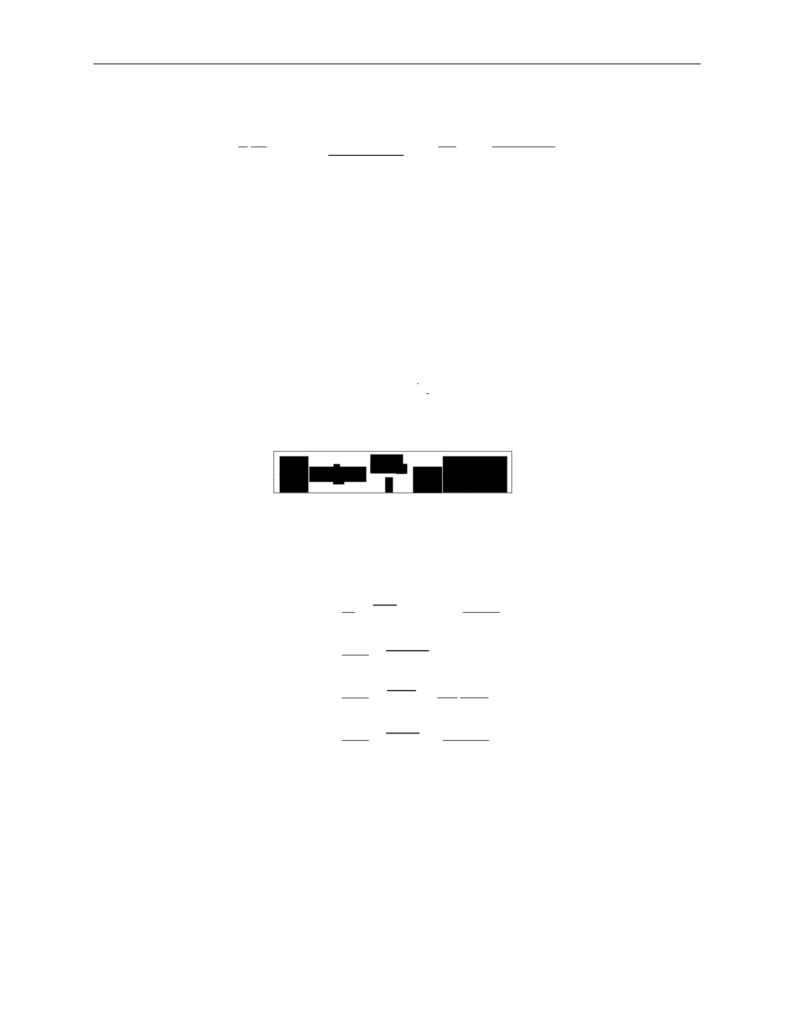
3.
MODELLING GALAXIES
43
2
2
2
2
t
t
t
— t
2
rr
rσ
rσ
rσ
rr
r
∂r
G
n
∂r
rr
—
dr
2
—
The simplified Jeans equation is:
1 ∂ 2(σ2
− σ ) ∂φ
GM (< r)
(nσ
2
) +
rr
t
=
−
=
−
(183)
where we’ve plugged in gravity as the force.
We have three limits we can look at:
•
σ
rr
•
σ
rr
•
σ
rr
σ
2
: nearly circular orbits
σ
2
: nearly radial orbits
= σ
2
: isotropic orbits
We define the anisotropy parameter:
σ
2
β
=
1
rr
(184)
which gives us a useful form of the Jeans equation for observations:
.
(185)
This depends only on radial components with uncertainty from
β
, assuming spherical sym-
metry and a steady-state system.
This can be simplified further to get mass estimates:
r2
1 ∂ 2 2βσ2
M (< r)
=
−
(nσ
)
+
2
=
−
rr
r
∂
(nσ
2
)
+
2β
G
2
=
rr
G
2
rr
r dn
+
n dr
rr
r
dσ
2
rr
+
2β
rr
(186)
2
=
rr
G
d ln n
+
d ln r
d ln σ2
rr
+
2β
d ln r
where the last line can be measured with observations.
Stability of stellar systems
The existence of equilibrium solutions to the collisionless Boltzmann equation does not assure
stability. Real stellar systems are subject to perturbations. What is important for stability?
Luminosity-velocity relations:
We can relate properties of a galaxy to observables through several equations:
1 ∂
2βσ2
σ
nσ
σ
n
∂r
r
2
r
∂r

3.
MODELLING GALAXIES
38
v
·
R
θ
=
(apparent size)
d
L
F
=
4πd
2
(158)
v
2
=
GM .
R
Introducing surface brightness Σ
F
L
d
2
Σ =
=
θ
2
4πd
2
R
2
(159)
L
v
4
then
=
4π
·
G2M 2
v
4
L =
Σ4πG
2
(M/L)
2
.
(160)
If we assume, for a given class of galaxies, that the surface brightness and the mass-to-light
ratio are the same, then
.
(161)
This introduces two important relations.
The Tully-Fischer relation is used for spiral galaxies and relates the maximum velocity in
the rotation curve
v
max
, which can be measured from HII spectra, and the luminosity:
4
max
.
(162)
The Faber-Jackson relation is used for ellipticals and relates the velocity dispersion
σ
v
to the
luminosity:
L
∝
σ
4
.
(163)
Thus, we can get an estimate of the intrinsic luminosity of a galaxy be measuring stel-
lar velocities. The constant of proportionality is roughly
L
∗
/(220 km/s)
4
, where
L
∗
is the
characteristic galaxy luminosity.
3.S
Phase-space distribution function
We have described the individual orbits in a potential, but this is not sufficient to describe
galactic dynamics. We want information of the configuration of all particles. Each star is
described by its position
→
x
and velocity
→
v
,
and we need to know this for all stars, i.e. how
stars are distributed in the 6D phase space
(
→
x
,
→
v
)
.
We define a phase-space distribution function
f
(
→
x
,
→
v
,
t)d3
→
x
d
3
→
v
(164)
∝
L
∝
v
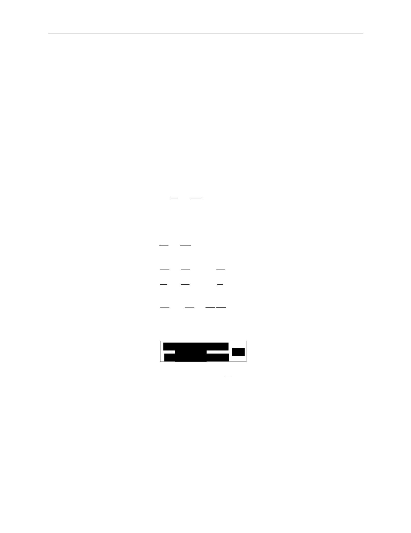
3.
MODELLING GALAXIES
39
∈
dt
as the probability that at time
t
, a randomly chosen star has
(
→
x
∗
,
→
v
∗
)
([
→
x
,
→
x
+
d
→
x
]
,
[
→
v
,
→
v
+
d
→
v])
.
This
means
that
the function must be normalized for all
t
, i.e.
∫
f
(
→
x
,
→
v
,
t)d
3
→
x
d
3
→
v
= 1 .
(165)
Collisionless
Boltzmann
equation
:
We want to describe the time evolution of
f
(
→
x
,
→
v
,
t)
. Since probability cannot be destroyed,
the 6D continuity equation must hold.
We define the 6D phase-space vector
then
w
→
=
(
→
x
,
→
v
)
(166)
∂f
+
∂
f
w
→
˙
=
0 .
(167)
∂t
∂w
→
This is the same form as the standard 3D continuity equation. We can rewrite this by
expanding out
w
→
and using velocity
→
v
=
→
x
˙
and acceleration
→
a
=
→
v
˙
:
0
= ∂f +
∂
f
w
→
˙
∂t
∂w
→
∂f
∂
=
+
∂t
∂
→
x
(
f
→
x
˙
) +
∂
(
f
→
v
˙
)
∂
→
v
(168)
∂f
∂
∂
=
+
(
f
→
v
)
+
f
(
−
∇
→
φ)
∂t
∂
→
x
∂
→
v
∂f
∂f
∂φ
∂f
=
∂t
+
→
v
∂
→
x
−
∂
→
x
∂
→
v
.
This gives us the collisionless Boltzmann equation (CBE):
.
(169)
Note that another way to see this is by writing out
df
= 0
and taking the limits
lim
→x
→∞
= 0
and
lim
→v
→∞
= 0
.
General Jeans equations:
A solution to the collisionless Boltzmann equation is difficult to obtain, so we instead study
moments of the CBE and the phase-space distribution.
Moments of the phase-space density give us some average quantities of the system.
a)
The first moment gives the density
n
of the system:
n
=
∫
f
d
3
→
v
.
(170)
∂t
−

3.
MODELLING GALAXIES
40
ij
∫
—
∫
∫
∫
±∞
—
i
n
i
i
j
n
i
j
∂
→
x
∂
→
v
∂
→
x
∂
→
v
∂
→
x
→v=
−∞
j
∂t
j
∂
→
x
j
∂
→
x
∂
→
v
2
b)
The second moment gives the average velocity
v
¯
i
:
v
¯
=
1
∫
v
f
d
3
→
v
.
(171)
c)
The third moment gives the velocity dispersion
σ
2
:
v v
=
1
∫
v v
f
d
3
→
v
ij
=
v
i
v
j
−
v
¯
i
v
¯
j
=
(v
i
−
v
¯
i
)(
v
j
−
v
¯
j
)
.
We now examine moments of the collisionless Boltzmann equation more closely. We break
each integral into three terms to simplify each individually.
gg)
First moment:
d
3
→
v
∂f
∂t
∂f
+
→
v
∂
→
x
∂φ
∂f
=
0
∂
→
x
∂
→
v
∫
d
3
→
v
∂f +
∫
d
3
→
v
→
v
∂f
−
∫
d
3
→
v
∂φ
∂f =
0 (173)
∂t
` ˛
1
¸ x
∂
→
x
` ˛
2
¸ x
∂
→
x
∂
→
v
` ˛
3
¸ x
:
d
3
→
v
∂f =
∂
∂t ∂t
d
3
→
v
f
=
∂n
∂t
:
d
3
→
v
→
v
∂f
∂
→
x
∂
=
∂
→
x
d3
→
v
→
v
f
=
∂
∂
→
x
n
→
v
¯
=
Σ
∂
∂x
i
(
n
v
¯
i
)
(174)
:
∫
d
3
→
v
∂φ
∂f
=
∂φ
∫
d
3
→
v
∂f
=
∂φ [f ]
→v=+
∞
=
0
For the third term, we used the fact that phase-space distribution goes to 0 at
for
physical systems.
This gives us the 3D continuity equation:
hh)
Second moment:
.
(175)
∫
d
3
→
v
vj
∂f
∂f
+
→
v
∂t
∂
→
x
∂φ
∂f
=
0
∂
→
x
∂
→
v
∫
d
3
→
v
v
∂f +
∫
d
3
→
v
v
→
v
∂f
−
∫
d
3
→
v
v
∂φ
∂f
=
0
(176)
` ˛
1
¸ x ` ˛
2
¸ x ` ˛
3
¸ x
1
2
3
∂n ∂
∂t
0
σ
∫
i
(172)

3.
MODELLING GALAXIES
41
ij
Σ
∫
i
∂x
∂x
j
∂t
∂t
j
∂t
j
∂t
∂t
∂x
i
∂t
∂t
j
∂x
i
using the continuity equation ∂n
=
−
Σ
∂
(
n
v
¯
)
j
∂
→
x
i
∂x
i
∂x
i
j
i
i
∂x
ij
i
j
∂x
j
∂v
j
v
i
=
−∞
i
∂v
∂t
∂x
i
∂x
ij
i
j
∂x
i
`
i
i
ij
i
∂x
i
∂v
:
∫
d
3
→
v
v
∂f =
∂
∫
d
3
→
v
v
f =
∂
(
n
v
¯
) =
∂
n
v
¯
+
n
∂
v
¯
j
=
−
v
¯
Σ
∂
(
n
v
¯
) +
n
∂
v
¯
j
=
n
∂
v
¯
j
−
v
¯
Σ
∂
(
n
v
¯
)
∂t
∂x
i
i
to go from the first line to the second
:
∫
d
3
→
v
v
→
v
∂f
=
∫
d
3
→
v
v
Σ
v
∂f =
Σ
∂
∫
d
3
→
v
v v
f
= nv
j
v
i
`
= n
˛ ¸
σ
2
+
x
v
¯
i
v
¯
j
=
Σ
∂
n
σ
2
+
v
¯
v
¯
:
∫
d
3
→
v
v
∂φ
∂f
=
∫
d
3
→
v
v
Σ
∂φ
∂f
=
Σ
∂φ
∫
d
3
→
v
v
∂f
(177)
((k, l, i) are permutations of (1, 2, 3))
=
∂φ
dv
∂x
k
∫
dv
l
∫
dv
i
∂f
v
j
∂v
=
[v
f
]
˛
v
¸
i
=+
∞
−
x
∫
dv ∂v
j
f
= 0
−
∫
dv
i
δ
ij
f
=
−
Σ
∂φ
∫
dv
∫
dv
l
∫
dv
i
δ
ij
f
i
i
=
−
Σ
∂φ
∫
d
3
→
v
δ
f
i
i
∂φ
=
−
n∂x
j
Plugging each term back in, we get
n
∂
v
¯
j
−
v
¯
Σ
∂
(
n
v
¯
) +
Σ
∂
n
σ
2
+
v
¯
v
¯
+
n
∂φ
=
0
(178)
i
i
i
i
i
i
i
i
i
i
i
1
2
3
j
j
i
j
i
i
j
∂
→
x
∂
→
v
j
i
i
i
j
k

