Introduction Biological affinity studies or geographic

Biological affinity studies or geographic population analyses have long been a focus

of anthropology. Archaeologists tend to approach this topic in terms descriptions of

prehistoric peoples and their migrations across the landscape through the analysis of the

material culture left behind. Linguists may examine population studies through changes

in word meaning, pronunciation, and language constructs. Physical anthropologists, and

more relevant to this dissertation, forensic anthropologists explore populations in terms of

identity, or biological groupings (frequently in terms of ethnicities or populations). As

physical anthropologists, determining the biological affinity of a group, or simply

classifying a single individual to a population, is a demanded skill – both from colleagues

in anthropology and professionals in the medico-legal community.

The goal of this dissertation is to provide an ―on the ground anthropologist‖ a suite

of tools by which to estimate biological affinity through the use of a relatively robust

bone, the mandible. It is intended also to present a method for determining the biological

affinity that is straightforward and easily understood (e.g. simple morphometric and

morphoscopic scoring methods), without the need for complex statistical manipulations

(they are provided). A byproduct of this study is the evaluation of the mandible in the

determination of the sex of an unknown individual. As the mandible is a relatively robust

skeletal element, it (or portions of it) can survive circumstances that other elements may

not. Not a complete mandible, but rather just portions of it, could be all that is needed for

accurate estimates of ancestry or sex. Further, if both morphometric and morphoscopic

features are employed at the same time, smaller and smaller portions of the bone are all

that may be needed to determine the biological profile of an individual. This dissertation

explores mandibular morphometric data, morphoscopic data, and the combination of both

for their potential to diagnose the partial biological profile of an unknown individual,

based on data from multiple world populations.

The Mandible

A brief review of mandibular architecture and function is provided, as it is the form,

which follows the function that is specifically analyzed in the bulk of this dissertation.

The primary functions of the adult mandible are to form the lower floor of the mouth, to

provide a vehicle for the growth and development of the lower dentition, and to provide

anchor points for the muscles of mastication. It is a complex bone and is the only bone of

the cranium to have independent movement other than the ear ossicles (Scheur and Black

2000). The principal portions of the mandible include the body (the horizontal ramus)

and the vertical (ascending) rami, the latter are divided into a triangular portion called the

coronoid process, a rounded articular eminence called the mandibular condyle. A final

feature of the adult mandible is the chin, which is a uniquely human feature (Bass 2005).

The mandible articulates with the cranial base, at the temporomandibular joints on the

temporal bones, through the mandibular condyles.

The mandible arises through endochondral ossification processes, beginning at

approximately the seventh week of intrauterine life; it is the second bone in the body to

begin ossification after the clavicle (Baker et al. 2005; Gray 1995; Scheur and Black

2000). The mandible begins ossification in two separate centers, one each in a

symmetrical half, both of which articulate together at the mandibular symphysis. An

extensive review of this ossification processes can be found in Scheur and Black (2000).

By the perinatal period, the mandible consists of the body and ascending ramus. The

ascending ramus is complete with the condylar and coronoid processes and is

approximately half the length of the body (Scheur and Black 2000). At birth, the tooth

crypts are present, as well as tooth germs. The mandibular hemispheres are united at the

mental symphysis by a fibrous tissue that fuses at approximately one year (Baker et al.

2005; Gray 1995).

After birth, the mandible undergoes more variations in shape and size than any other

facial bone in order to maintain proper growth trajectories with the maxilla, cranial base,

and the dentition (Enlow and Hans 1996; Scheur and Black 2000). The mandibular

condyle plays an important role in this process, due to downward and forward movement

from the cranial base, but also the modeling and remodeling of the entire ramus is

responsible for these actions (Enlow and Hans 1996). Overall, the modeling and

remodeling experienced in the months and years after birth reduce the mandibular angle

from approximately 175 degrees to around 130 degrees (Gray 1995; Scheur and Black

2000). The chin rapidly changes, increasing in size and depth to make way for the

developing dentition, as does the alveolar process. The body elongates, particularly

behind the mental foramen to provide space for the developing distal dentition (Gray

1995). Sexual dimorphism starts to appear in the mandible around puberty, though it is

argued that since most growth and development is completed earlier in childhood, sexual

dimorphism should be apparent in younger individuals as well. While some studies have

argued this point (see Humphrey, 1998; Molleson et al. 1998), it is far from readily

proven.

The mandible has the anchoring points for the muscles of mastication, but this

musculature is also responsible for many other activities. Specifically, the mandibular

musculature maintains the airway, is responsible for the gag reflex, provides for infant

suckling and swallowing, and allows for speech and facial expressions (Enlow and Hans

1996). The muscles most obviously associated with the mandible are the masseter and

temporalis, which attach on the lateral aspect of the ascending ramus and the superior and

medial surfaces of the coronoid process. Equally important and often unmentioned

muscles associated with mastication, facial movements, speech, are those found on the

medial mandibular surface such as the superior pharyngeal constrictor, medial and lateral

pterygoids, mylohyoid, digastric, genioglossus and geniohyoid muscles. Without these

small, but important muscles, the floor of the mouth, speech, and chewing would not be

possible. Each of the muscles attaches to a various ridge, spine, fossa, process, etc. that

often play a part in the specific traits and measurements analyzed in this study.

Biological Affinity and Its Diagnosis: The Problem

Frequently, an individual’s biological affinity is labeled as that person’s ―race.‖

Defining the term race has been extremely difficult in anthropology simply because racial

identity often is based on a multifaceted construct of characters such as social identity,

ethnic identity, and the body’s phenotypic configuration. A discourse of the various

viewpoints on the term race is beyond the scope of this dissertation; however, suffice it to

note that physical anthropology recognizes that there are no pure human ―races‖ (AAPA

1996). A dichotomy exists between what is scientifically recognized and the practical

application of physical anthropology in modern forensic situations. Physical and forensic

anthropologists frequently are asked to make statements about the race of an unknown

individual by police agencies, medical examiners, and government officials in the pursuit

of the identity of an unknown person. Indeed, the U.S. government categorizes persons

based on their race in a manner proscribed by the Executive Office of the President of the

United States, Office of Management and Budget. Directive 15 published on October 30,

1997, with an effective date of January 1, 2003, states that the federal government

recognizes six racial groups (or a minimum of five racial groups and two ethnicities).

These are American Indian or Alaska Native, Asian, Black or African American, Hispanic

or Latino, Native Hawaiian or Other Pacific Islander, and White; the government

specifically states that these labels do not necessarily correlate to biological or genetic

underpinnings (Federal Register Notice, 1997).

The idea of race is important to law enforcement and medical professionals (it is part

of the foundation for identity in the United States), although the concept of discrete races

are not accepted scientifically. Even for the average person in today’s society, predefined

social, socio-economic, and biological connotations are associated with a given race. It is

the dichotomy between the scientific and social concepts that arguably has led to the

continued use of the term race and it may be why many recent introductory textbooks to

physical and forensic anthropology and scientific publications continue to use the term.

Even though the use of the word ―race‖ is commonplace, the terms biological affinity,

geographic population, or ancestry are used to describe the biological origins (perceived,

estimated, or real) of a given individual or population, rather than race, where possible.

This study presupposes that the determination of the biological affiliation of an

individual is an extremely important aspect of an anthropologist’s workload, particularly

for those in a forensic setting. The ability to determine the biological affinity of unknown

human remains often narrows the possibilities of who that individual was, helping lead to

a positive identification. The genetic make-up of any given individual is an

amalgamation of their parents, their parents’ parents, and so on, who frequently shared a

geographical population (particularly before the advent of modern travel conveniences).

This geographic background is taken into account when determining aspects of skeletal

biology, such as stature (Ross and Konigsberg 1999; Trotter and Gleser 1952) and age

(Berg 2004, in press; Katz and Suchey 1989; Prince and Ubelaker 2002; Schaefer 2004).

The need for population specific estimation methods for age and stature are increasingly

pointed out in the literature (see Hoppa 2000; Komar 2003), which obviously questions

how good are estimation techniques for biological affinity and what techniques are

available to the anthropologist. Without a strong and accurate assessment of biological

affinity, other skeletal determinations can be inaccurately estimated.

Anthropologists’ ability to accurately diagnose the biological affinity of an unknown

set of human remains is somewhat limited. Physical anthropologists typically utilize

craniofacial traits and dental morphology to determine the biological affiliation of a given

set of remains (e.g. Brues 1990; Edgar 2005; Gill 1986; Krogman 1962; Rhine 1990;

Stewart 1979). Unfortunately, the fragile facial bones and teeth are frequently missing,

damaged, or destroyed due to trauma or taphonomy, particularly in cases such as

vehicular accidents, skeletonized remains (particularly in outdoor, above ground

environments), intentional mutilation, and in archaeological contexts. Metric cranial

analyses, including univariate (e.g. Hanihara 2000) and multivariate (Burris and Harris

1998; Byers et al. 1997; Holland 1986; Howells 1973; Jantz 1973; Key and Jantz 1990;

and Owsley and Jantz 1977) methods are another tool for determining population affinity.

Few studies attempt to analyze large world populations and typically only focus on two to

three groups. While often statistically more robust than morphoscopic applications, these

types of analyses suffer from the same problems that plague cranial morphoscopic

analyses.

Postcranial methods for determining population affinity are particularly lacking. A

few studies on the femur currently exist (Baker et al. 1990; Gilbert and Gill 1990; Stewart

1979), but are rarely employed in forensic cases, simply due to the limited variety of

populations that are represented. A radiographic approach using the femoral

intercondylar shelf angle (Craig 1990) to determine White or Black ancestry for an

unknown femur has recently been shown to be problematic (Berg et al. 2007). A

somewhat recent study was published on the utility of determining the sex and population

group from the bones of the hand (Smith 1996). In addition to these methods, the

computer programs FORDISC 2.0 or 3.0 (Ousley and Jantz 1996; Jantz and Ousley 2005)

are frequently used to assess the biological affinity of postcranial elements for U.S. Black

and White individuals through the creation of custom discriminant functions for desired

measurements.

The problem of determining population affiliation is stated eloquently by White and

Folkens (2005:403):

―Even with this element (the cranium), all workers agree that racial estimations are

usually more difficult, less precise, and less reliable than estimations of age, sex, or

stature. Despite decades of research, much more osteological work on geographic

differentiation with Homo sapiens remains to be done and is urgently needed.‖ Their

statement may be interpreted to be a bit extreme (except for the last point), but their

early points are often echoed by the choice of content provided by the authors of

several recent basic physical anthropology and forensic textbooks. Examination of

the table of contents within these texts gives the general impression that biological

affinity is something best left to others, or, at the minimum, is a very troubling topic.

White and Folkens (2005) devote four pages to the determination of ancestry yet have

22 pages on estimation of age and 13 pages on the estimation of sex. In the

introductory Forensic Anthropology Training Manual by Burns (1999), the

determination of race is discussed on three pages, whereas sex, stature, and age are

discussed on a multitude of pages in relation to many of the individual bones and

teeth that play a part in their estimation; to be fair, racial analysis of the skull is one of

the three aforementioned pages. Pickering and Bachman (1997) detail various

osteological analyses in their introductory text as well. While listed nearly first in the

order of basic anthropological operations to undertake, their section on race, ethnicity,

or cultural affiliation, is one and a half pages long. Discussion of sex is five and a

half pages and age also is given a similar amount. Finally, in their chapter on skeletal

tissues in the book Forensic Human Identification, Scheuer and Black (2007) allocate

two paragraphs to the determination of ethnic identity, yet spend three pages on

determination of sex and seven pages on age-at-death. In three of four of these texts

the largest contributor to the allocated space is tabularized information from Gill

(1995) and Rhine (1990) or Krogman (1962) on cranial morphology and racial

assessment. The lack of text in these books suggests several rudimentary problems:

1) Anthropologists do not have enough techniques with which to estimate biological

affinity;

2) It is too difficult for the introductory student/practitioner to estimate biological

affinity, thus little time will be spent on it;

3) The types of metric analyses that are present in the literature are complicated and

require specialized tools/data sets and therefore are not very usable to the

common ―anthropologist on the ground;‖

4) The techniques present are not valid (in the author’s minds) to warrant detailed

mention,

5) Perhaps there is some aversion to or unfamiliarity with metric analysis of the

human skeleton for biological affiliation;

6) The majority of the previously reported cranial metric analyses are specific to

small, forensically uninteresting populations;

7) And finally, timid anthropologists might shy away from such a contentious issue

(i.e. the whole ―race‖ debate), particularly in an introductory setting.

Which of these problems, or a combination thereof, is actually the correct answer is up

for debate.

Previous Mandibular Studies

Researchers have used mandibular morphoscopic and morphometric data to classify

and describe populations, but analyses of three or more groups (either morphometric or

morphoscopic) are rarely available. Early papers on mandibular morphometrics include

those by Harrower (1928), Hrdlicka (1940), and Morant (1936). Interest in the mandible

waned through the intervening decades, except for Giles (1964) work with discriminant

functions and sex determination. The early 1980s to the 1990s saw increasing interest in

the mandible. Kile (1983) used mandibular morphometrics to classify U.S. Whites and

Blacks, to include those of unknown biological affinity. Some of the most widely known

and cited works include papers by Angel and Kelley (1990) and Rhine (1990), which

utilized few populations or solely examined morphoscopic traits. Humphrey et al. (1999)

found that mandibular morphometric variables were poor discriminators of recent human

groups. Berg (2001, 2006) has explored mandibular morphoscopic traits between large

groups of individuals, as well as the ability to use discriminant function analysis to

achieve population classifications. The results of 3-D geometric morphometric analyses

to explore the shape of the mandible in relation to population groupings have recently

been published (Buck and Vidarsdottir 2004; Nicholson and Harvati 2006).

Older studies examined different populations using mandibular morphometrics (e.g.

Harrower 1928; Hrdlicka 1940; Morant 1936). These studies often used nonstandardized

measurements, relied heavily on indices, and frequently reported summary data rather

than raw data. These studies were undertaken in the infancy of anthropology, when the

focus was not so much on identifying an unknown individual as it was in characterizing a

population. Comparisons between large numbers of groups were not typical pursuits until

the latter part of the century; human biological variation studies incorporating mandibular

morphometrics or characteristics then started in earnest (Carlson and Van Gerven 1977;

Corruccini 1974; Hauser and De Stefano 1989; Schendel et al. 1980). These studies were

mostly focused on the cranial vault and face rather than the mandible, though a few traits

or measurements were incorporated (e.g. mandibular tori, mylohyoid bridging, rocker

jaw).

Kile (1983) examined the metric differences between equal numbers of male and

female American White and Black mandibles from the Terry collection (using 25

variables). Nine discriminant functions were determined for the data; all but one was

used to separate both sex and biological affinity. The functions were designed to utilize

sections of the mandible in most cases, rather than a complete specimen, or areas that

were determined to be population specific based on his observations. The last function

was developed solely to determine American Whites from U.S. Blacks, regardless of sex.

Discrimination ability ranged between 38.5% and 76.9%, depending on the variables

used. From the data, Kile determined that functions utilizing the corpus and ramus, or

variables that had high individual coefficients produced the best results. This work

remains as an unpublished master’s thesis.

Two papers appeared in Gill and Rhine (1990) concerning the mandible. Angel and

Kelley’s (1990) contribution explored biological affinity based on morphoscopic

attributes of the posterior edge of the ascending ramus (posterior jaw ramus border

inversion), as well as gonial angle eversion (or flare). Both traits were visually scored on

a scale of absent, slight, +, or ++. Their sample was derived from multiple collections,

though it was drawn predominately from the Terry collection. They found that the

posterior edge was a viable population discriminator between American Black and White

individuals, and from American Blacks and Native Americans. Some 70% of all of their

American White individuals lacked the posterior edge eversion trait, while 95% of their

American Black individuals expressed the trait. Gonial angle flare was found not to be as

population specific. From the presented information, it also appears that they quantified

their categorical data, likely as 1, 2, 3, and 4, to determine population means of the

morphological traits. The means were compared in some fashion (t-test?) to determine if

there were significant differences between American Blacks and Whites, likely by sex,

and the results are presented as p-values.

Angel and Kelley (1990) also explored some metric differences between the

American Black and White populations. Within the metric analysis, six mandibular

measurements were analyzed (mandibular angle, minimum ramus breadth, ramus height,

bigonial breadth, bicondylar breadth, and mandibular length). Of these, several were

found to be significantly different between groups (male/female, Black/White), but their

choice of statistic and their comparisons are not detailed. It is likely that the comparisons

are between Black and White males and Black and White females. Instead of producing

ways of separating the individuals based on results of the metric analyses, the authors

primarily used them to explain a probable genetic underpinning for the observed

morphology of the ascending ramus.

Rhine (1990) used limited samples and created generalized statements about

mandibular morphoscopic traits for four populations thusly labeled: Anglo, Black,

Indian, and Hispanic. The Anglos were composed of those of European origin, the

Blacks were likely contemporary U.S. Blacks, Hispanics were likely those of southern

European ancestry mixed with a number of Indian tribes, and the Indians were both

modern and prehistoric southwest Amerindians. The majority of his conclusions and

generalizations were based on extremely small sample sizes for the mandibular traits

(Anglo = 51, Hispanic = 8, Black = 3, Indian = 3). His generalizations have been taken to

heart by the anthropological community, and are often found in lists of racial traits in

forensic textbooks and other publications (Burns 1999; Byers 2002; Gill 1995; White and

Folkens 2005). The lack of sufficient sample size, particularly for the Amerindian and

Black categories, makes the regurgitation of his data in modern texts particularly

disconcerting (even though he warned of a small sample size problem). Complicating the

picture, Rhine’s morphoscopic data have been changed through time from

―Southwestern

Mongoloids (American Indian)‖ to ―Asians‖, at least in one current forensic text

(Byers 2002:154, 167).

Humphrey and coworkers (1999) examined a large collection of modern human and

great ape mandibles using 13 measurements. Of the measurements, four are considered

standard measurements in the forensic literature (e.g. Buikstra and Ubelaker 1994;

Moore-Jansen 1994), and nine were specifically designed for the study. Both univariate

and multivariate [principal components analysis (PCA), discriminant function analysis]

statistical methods were employed to analyze the data toward three goals: 1) interspecific

variation, 2) sexual dimorphism, and 3) regional and population variation in modern

humans. Population selection targeted the five major geographical regions, and though

the sample sizes often reached 30 individuals, some were lower, and no population

samples had over 30 males and females. Specifically for their third question, they found

high intraspecific diversity with no obvious regional patterning via basic statistical

analysis, and a weak regional pattern using PCA. But their conclusion does not seem to

be quite so warranted given that discriminant function analysis did assign 78.4% of the

mandibles to the correct geographical region, and 73.4% of all mandibles were correctly

assigned to a specific population. The conclusion that the mandible is not a ―good‖

discriminator of modern human populations appears to be derived more from

comparisons with cranial metrics that achieve a higher classification rate (93% overall

accuracy for the cranial vault), although the cranial metric studies used more variables

and only achieved a 20% increase in accuracy. In general, it seems that their conclusion

can be summed up as ―it is perhaps inevitable that the mandible will be less useful than

the cranium for identifying the relationships between human populations given this (its)

plasticity‖ (Humphrey et al. 1999:511).

Berg (2001) presented a large mandibular non-metric data set with the intent of

reexamining the generalizations presented by Rhine (1990). The paper examined seven

morphoscopic traits from three distinct populations: Cambodians, U.S. Whites, and

Nubians. Only males were included in the assessment, and some data (Native American,

and a portion of the U.S. Whites) were taken from the Rhine (1990) and Angel and Kelley

(1990) publications for comparison purposes. The scoring of several non-metric traits

was modified from the original descriptions (Angel and Kelley 1990; Rhine 1990) after

categorical differences were observed. The data showed that it was incorrect to assume

that Native American data could be substituted for Asian populations. The rates of

various morphoscopic states, such as the lower border of the mandible for American

Blacks and chin shape for Asians and American Blacks, were found to be significantly

different from those reported by Rhine (1990).

In a follow-up paper, Berg (2006) demonstrated the utility of constructing

discriminant functions for determining population affinity based on morphoscopic scores.

Research conducted by Ousley and Hefner (2005) showed that cranial non-metric traits

(as ordinal data) could reliably be used in linear discriminant functions to determine

ancestry. They reported that in-depth statistical analyses did not yield substantial

objections concerning the application of the discriminant functions to their ordinal data.

Following this logic, Berg (2006) treated the mandibular non-metric trait scores as ordinal

variables and constructed linear discriminant functions for multiple populations. Over

1000 individuals were used in the analysis; functions were constructed not only using two

group comparisons, but also three to seven group comparisons. Each analysis was cross-

validated (leave-one-out method) for accuracy assessment. The only variable to typically

be removed from the analyses was the ascending ramus profile shape. Seven population

comparisons yielded a 48% cross-validated accuracy rate, approximately three times

better than random expectation. Two group comparisons fared better, some in excess of

90%, while three group comparisons approached 70% accuracy rates. Further, two group

comparisons of closely related populations had viable functions, some with 74% cross-

validated accuracy rates.

Morphometric analysis of mandibles is an underrepresented technique in forensic

anthropology. Analyses of large population groups for mandibular morphometrics are

rare. Comparative mandibular data are available for American Blacks, Whites, and

Japanese in FORDISC 2.0 (Ousley and Jantz 1996). Mandibular metric data are not

present for the other comparative populations. The FORDISC 2.0 database comprises

individuals from multiple populations from the continental U.S., to include Terry

collection specimens with birth years after 1900, and a selection of 100 Japanese males

and females, courtesy of Hanihara and Hajime Ishida. Ten standard mandibular

measurements are available for custom-generated discriminant functions, though several

measurements are unavailable for the Japanese data. FORDISC 3.0 has similar

populations, though a Guatemalan population has been added (Jantz and Ousley 2005).

Buck and Vidarsdottir (2004) discuss the use of three-dimensional geometric

morphometrics as a method of determining the racial identity of sub-adult individuals

using three-dimensional coordinates obtained for 17 homologous landmarks of the

mandible. In their analysis, five populations were considered: African Americans,

Native Americans (Arikara), Caucasians, Inuit, and Pacific Islanders (total sample size

was 174 individuals). After employing generalized Procrustes analysis to superimpose

and scale the coordinate data to centroid size, principal components analyses,

Mahalanobis distance analyses, and cross-validated discriminant analyses were

conducted. In the first portion of their analysis, they found that the cross-validated linear

discriminant functions produced an average 70.1% accuracy rate for the five populations

(or three times chance alone). Using only three populations, African Americans,

Caucasians, and Native Americans, the cross-validated accuracy rate was 87.6%. To

determine if the method could be applied to partial skeletal material, the landmark data

were divided into two series, those that dealt with the corpus and those that were related

to the ramus. Again using the three groups, they found that the corpus could accurately

predict race with 67% accuracy, while the ramus accurately predicted the group

membership 73% of the time.

A poster presented at the American Academy of Forensic Sciences Annual Meeting

examined mandibular and other measurements of the dental arcade from American Black

and White mandibles (Danforth 2005). Eighteen measurements were taken on 183

American Black and White individuals from the Terry Collection. Of the measurements,

ten were standard and the remaining eight were defined specifically for the project.

Danforth (2005) reported that five measurements (M2-prosthion length, bigonial breadth,

minimum ramus breadth, alveolar length, and ramus height) consistently entered into

functions that discriminated between American Blacks and Whites (and between sexes as

well). Her functions had accuracy rates of 75.3% for the entire sample, 86.2% for males

only, and 93% for females only (female sample sizes were small).

Nicholson and Harvati (2006) discuss the use of three-dimensional geometric

morphometrics in relation to mandibular shape using three-dimensional coordinates

obtained for 28 landmarks. Their principal aim was directed at modern human origins

debates, rather than a forensic application. The sample included 155 mandibles from

broad regions of the world, though no sample population contained more than 26

individuals (a European population sample had the greatest number). Sex was unknown

in most cases; therefore their study sample was pooled. Their analysis utilized

generalized Procrustes analysis, which produced group centroids devoid of size (essential

for a ―shape‖ analysis). Additional analyses utilizing principal coordinates analysis,

Mahalanobis D2 statistic, multiple regression analysis, and discriminant analysis were

conducted. Ultimately, the authors determined that geographic patterning is present in

recent human mandibular shape, though there is considerable overlap. Their

classification rates were approximately 84% (by re-substitution), and several

climatological patterns were identified. As acknowledged by the authors, the study

suffers from small sample sizes within populations and their findings become less clear at

the fine-grained geographical scale.

Racial Mating Trends in the United States

A brief discussion on racial mating trends is appropriate here, as it is these patterns

that either maintain or create the patterns seen in human skeletal variation. According to

the National Center for Health Statistics, Division of Vital Statistics, interracial marriages

are rare. Indeed, the percentage of interracial marriages during the period of 1963-1967

averaged only 1.1% (Hetzel and Cappetta 1971). This percentage may be artificially low

as only 35 states tracked the racial category of individuals on marriage registrations. A

recent review of the U.S. Census data shows a growth trend in interracial marriages, from

0.4 percent in 1960 to 2.2% in 1992 (U.S. Bureau of the Census 1998). This indicates

that the Division of Vital Statistics data are likely a good estimate for its time period as

well. Although interracial marriages account for a small fraction of the all marriages in

the United States, the amount of racial admixture in U.S. populations is greater (if

migration rates are held constant), since admixture is an likely an additive process

through time (per generation).

The effect admixture has on skeletal morphology can be a difficult question to

answer. The question is compounded by the fact that ―race‖ is frequently self-reported

and it is based on the social group an individual ascribes to. Skeletally, an individual may

be determined to be ―Black‖ by an anthropologist, but that individual is ascribed to a

―White‖ racial group. More difficult is the ―Hispanic‖ racial group, as these individuals

may ascribe to being White, Black, Latino, or Native American. Therefore, measuring

the effect of admixture on skeletal traits becomes exceedingly difficult in the absence of

genetic data.

Genetic data do shed light on the admixture problem in skeletal biology, in that it can

potentially be used to ―inform‖ the anthropologist of the likelihood of finding ancestral

traits of one group expressed in an individual of another. But the actual genetic makeup

of any one phenotypic trait commonly used by skeletal biologists has not been

determined. Instead, the amount of admixture of various groups has been reported, and it

is this data that may be helpful in the future. Parra et al. (2001) found that the amount of

European admixture in African American populations for several rural populations in

South Carolina was approximately 12%, though for a more urban sample from Columbia,

the percentage of admixture was higher, at 18%. The urban figures compared well with

studies conducted in populations from urban settings such as New York (20%), Baltimore

(16%), and Detroit (16%) (Parra et al. 1998). African American admixture into European

populations is definitively smaller. A study conducted by Shriver et al. (2003) showed

that a group of European Americans from State College, Pennsylvania had a higher

admixture component of Native American genes (3.2%) than African American genes

(0.7%).

Two other interesting points are noted: first, the majority of the admixture into

African American populations by European Whites is contributed by males, a fact that fits

well with American slavery practices (Parra et al. 1998). Second, the amount of genetic

change in the African American populations is increasing. Relatively closed groups have

retained smaller amounts of admixture, ~11%, while populations from more urban and

potentially more open mating situations have increased to ~20%. Parra et al. (1998)

suggest one possible explanation for this change in admixture frequency is from a large

migration of African American populations from the south to the north after World War I.

Given this hypothesis, a rough estimate of the admixture amount in these populations per

generation could be calculated. The estimated generational increase in admixture is about

3% (9% over three generations) for African American populations, if the hypothesis of

Parra et al. (1998) is correct.

What does this mean to the physical anthropologist? Potentially it means is that we

could see more ―White‖ traits expressed skeletally in individuals of ―Black‖ ancestry

than is expected in a ―pure‖ ancestral line. Also, traits found more frequently in Native

American populations would likely be found in White populations. Further, this pattern

would likely grow with time, until a genetic balance is achieved, if that can actually

happen. If admixture is an additive process, then physical anthropologists should

continue to see a dilution of absolute phenotypic expressions and a change through time

toward a moderate or midline phenotypic state.

This brief review illustrates that there is a continued need for detailed study of the

mandible, particularly emphasizing populations other than American Blacks and Whites,

which are usually from the Terry collection. This dissertation places a particular

emphasis on those that are forensically relevant to today’s U.S. population as well as

consider a diverse set of world-wide groups. As was noted, several studies using world

populations have been conducted, and the ability to discriminate between them is robust,

albeit not quite that of cranial metric analyses. While variability in some of the previous

results is the norm, the notion that the mandible is a poor discriminator of recent human

groups appears unfounded. The results of this study will contribute to this particular

argument. Furthermore, a combined analysis of morphometric and morphoscopic data

from the mandible may provide better classification rates than have been achieved to

date.

Chapter 2

Materials and Methods

The majority of forensic methods for determining biological affinity have focused on

the differences between American White and Black populations, largely based on skeletal

material from the Robert J. Terry collection. Studies focusing only on these two

population samples obviously suffer in their applications considering the diverse

population currently living in the United States. Table 1 lists the recent population

characteristics for the country. As seen, over 20% of the U.S. population is neither White

nor Black. But the census data are only a portion of the ―forensic‖ picture that should be

considered. Recent statistics from the U.S. Department of Justice (Rennison 2001) give

the specifics for those involved in, or are victims of, violent crime. Current homicide

data from Los Angeles County (Leovy et al. 2007) also shed light on the forensic picture

(Table 1). These data demonstrate that if forensic personnel only considered American

White and Black populations, they would substantially underestimate numbers of

―other‖ individuals who find themselves in violent and dangerous situations. While not

listed in Table 1, the historic homicide rates for all racial categories averaged across the

country are approximately the same (~5 per 100,000), except for Black individuals, who

are six times more likely to be murdered than White individuals, and eight times more

likely than people of other races (Rennison 2001). The Los Angeles County data show a

higher prevalence of homicide rates involving Blacks and Hispanics. In general, since

those involved in violent crime arguably have a higher likelihood of becoming a forensic

case, developing biological affinity models for only U.S. Whites and Blacks is short-

sighted.

Table 1. Population characteristics of the United States and population characteristics of

those involved in violent crime from across the country.

Population Percent

Average number

of incidents per

1000 individuals

Homicides rates per

100,000 individuals,

Los Angeles County

White 65.0 60.9 3.2

Black 14.0 83.7 34.0

Hispanic 13.0 59.0 11.2

Asian 4.6 38.0 2.7

American Indian 2.0 173.8 n/a

Other 1.4 n/a 10.1

Population Samples

The need to develop more methods for assessing biological affinity from diverse

populations is clear. Bearing this in mind, multiple samples from world populations were

gathered for this study. Table 2 lists the study samples broken down by sex and sample

size. With a perusal of Table 2, the reader may assume that some of the populations are

not forensically relevant; this is not the case since prehistoric Native American remains,

trophy skulls, and other unusual cases are presented to forensic investigators as recent

forensic cases with certain regularity.

The mandibular data were collected over a period of approximately four years in a

variety of world-wide locations, from the Killing Fields of Cambodia to laboratories

containing the results of recent mass grave excavations in Guatemala and at the various

collections housed at the Smithsonian Institution. Many of the collections are well

documented and contain information on age, sex, stature, and ancestry. In other

instances, the biological data were determined through osteological analysis. No

juveniles are included in the study. The justifications for lumped categories, such as

Hispanics, are discussed and each sample is described more fully below.

Terry collection (U.S. White and Black samples)

Mandibular data for U.S. Whites and Blacks were gathered at the Terry collection,

housed at the Smithsonian Institution, Washington, D.C. The Terry collection was

procured by Dr. Robert Terry in St. Louis, primarily between 1910 and 1941, though Dr.

Mildred Trotter continued to add to the collection until near her retirement in 1967. The

collection is comprised of primarily U.S. Whites and Blacks, and records documenting

the sex, age, race, and cause of death are available. Birth years are primarily between

Table 2. The study sample, by collection and sex.

Samples Males Females Total

U.S. Whites, Terry collection 55 6 61

U.S. Whites, William Bass collection 125 56 181

U.S. Whites, CIL collection 22 0 22

U.S. Blacks, Terry collection 55 55 110

U.S. Blacks, William Bass collection 27 3 30

U.S. Blacks, Memphis collection 15 13 28

Hispanics, William Bass/PCME collections 30 1 31

Guatemalans, FAFG collection 89 14 103

Vietnamese, CIL collection 42 1 43

Chinese, CIL and Hrdlicka collections 65 1 66

Cambodian sample 149 29 178

Prehistoric Hohokam, ASU/Hrdlicka collections 35 14 49

Proto-historic Arikara, UT collection 30 30 60

Prehistoric Nubians, ASU collection 56 55 111

Total: 795 277 1072

1822 and 1943 (the data in this study represent individuals with predominately 19th

century birth years). While efforts were made to select for complete, toothed mandibles

and documented ages, no other criteria were used in the selection process. A minimum of

55 individuals was collected for both population samples and sexes, with the exception of

White females, which are sadly underrepresented since most in the collection were

edentulous.

William W. Bass Donated collection (U.S. White, Black, and Hispanic samples)

The William W. Bass Donated collection began in the early 1980’s and is composed

of individuals who specifically donated their remains to the University of Tennessee,

Department of Anthropology. Individuals are allowed to decompose on several acres of

land at the Anthropology Research Facility, after which the remains are cleaned,

measured, and curated. The size of the collection is slightly over 1000 individuals, nearly

all of which have documented sex, age, stature, and cause/manner of death. The birth

years range for the collection is from 1892-1987, with the vast majority falling between

the years 1915 and 1962 (20th century birth years). In addition to this collection, a few

specimens were selected for analysis from the University of Tennessee Anthropology

Department’s Forensic collection. The majority of the individuals collected for this study

had known ages, though a few only had age ranges. Black and Hispanic individuals are

poorly represented in the collection, and White females were not as commonly

encountered as White males. The Hispanic data were combined with those from the

Pima County Medical Examiner collection (see below).

Memphis collection (U.S. Black sample)

This sample stems from a cultural resource management archaeological excavation of

an American Black cemetery in Shelby County, Tennessee (Oster et al. 2005). The

cemetery was in use ca. 1899 to 1933. Given the adult status of these individuals, and the

dates of the graveyard, the likely birth years for these individuals are between 1840 and

1900 (19th century birth years). All of the selected mandibles had confident sex

assignments from osteological findings and all ages were based on osteological

assignment. Additional osteological information on this collection can be found in

Meadows-Jantz and Wilson (2005). In the remainder of the study this sample was

combined with the Terry collection sample, based on the birth years of both groups.

Central Identification Laboratory (CIL) collections (U.S. Whites, Vietnamese, and

Chinese samples)

Samples from three populations were obtained from the CIL at Hickam Airforce

Base, Hawaii. The first is a small sample of U.S. war dead predominately from World

War II and the Korean War. All of these White male individuals have been identified and

have known ages-at-death. The majority were young, between 19 and 28 years at death.

The span of birth years is between 1901 and 1936, with the majority between 1917 and

1932. One casualty from the Vietnam War is in the study; he also is the oldest individual,

49 years of age, and was born in 1936. All of these individuals have been repatriated

back to their respective families. For all forthcoming statistical evaluations, these

individuals were combined with the William W. Bass Donated collection sample

(20th century birth years).

The second sample is a large group of Vietnamese males who were aboard a C-130

aircraft that crashed in 1974, during the Vietnam War. All individuals aboard the aircraft

were male, and of ―fighting age.‖ All are aged as ―adult,‖ and none appeared to be

older than 50 years or younger than approximately 20 years. Based on this assessment,

the likely birth years for these individuals is between 1925 and 1955. In addition to the

single crash incident, multiple sets of remains, which have been identified as Vietnamese,

are housed at the laboratory. All sex and age estimates of these individuals are derived

from osteological analysis, and several are aged merely as adult. One female is

represented in this latter group. Although nearly impossible to determine, the birth years

for these individuals are likely similar to those involved in the C-130 crash, or slightly

older.

The final sample is a small group of likely Chinese individuals (n=9) that have been

recovered by CIL anthropologists during excavations on the Korean peninsula, usually

north of the 53rd parallel. All associated cultural materials were Chinese in origin (e.g.

buttons, clothing, and military equipment). The excavation locations are consistent with

Chinese military engagements with U.N. troops (e.g. the Chosin Reservoir area). When

available, cranial-metric analysis using FORDISC 2.0 (Ousley and Jantz 1996) was

conducted and each classified as a Chinese male. While it is possible that one or more of

these individuals is actually a Korean, all available evidence indicates a Chinese origin.

Therefore, these data were combined with the Hrdlicka Chinese sample (see below).

Pima County Medical Examiner (PCME) collection (Hispanic sample)

The PCME office has a relatively small, rotating collection of unidentified human

remains that have been found in the desert between roughly Tucson, Arizona and the

U.S./Mexico border (Bruce Anderson, pers. comm. 2004). Frequently, the remains have

been found by hunters/hikers and are in a skeletonized condition. Undoubtedly, these

remains represent those individuals that attempted to cross the border into the U.S. and

failed to find safety. Roughly once a year, the unidentified remains are buried in a

common grave by county officials. While identifying their biological affinity currently is

difficult, anthropological analysis typically classifies them as Hispanic; eight individuals

have been identified positively as Mexican nationals and the rest are held in a status of

unidentified border crossers (Bruce Anderson, pers. comm. 2007). All of the biological

data from this sample are from osteological analysis (most individuals are

complete/nearly complete skeletons). All but one individual were males. Given their

classification, these individuals and those identified as Hispanics from the William Bass

collection have been grouped together as Hispanics.

Fundacion de Antropologia Forense de Guatemala (FAFG) collection (Guatemala Maya

sample)

The FAFG is an organization in Guatemala dedicated to the recovery and

identification of those individuals that were killed during a brutal, multiple-decade civil

war. Their collections are rapidly rotating; as individuals or groups of individuals are

identified, their remains are returned to the appropriate village for internment. As would

be expected from a civil war environment, the majority of the remains are those of males,

though females and children are often recovered. All sex and age estimates are from

osteological analysis by FAFG anthropologists. Females are under-represented in this

sample. The individuals comprising this particular sample were from several villages

from the country’s interior and can be considered indigenous Indians (Mayan). Broken

or missing mandibular portions due to taphonomy (e.g. crushing, warping, erosion) or

trauma (e.g. projectile damage) were frequently encountered, and where possible, still

scored and measured.

Chinese sample

The Chinese sample is comprised of two groups, the CIL Chinese collection detailed

above, and a sample from a Chinese cemetery in Uyak Bay, Kodiak Island excavated by

A. Hrdlicka in 1931 (Hrdlicka 1944). These individuals were ―hired‖ to work in the

canneries on Kodiak Island in the late 1800s (Dave Hunt 2007, pers. comm.). These

individuals are thought to be labeled the ―Canton District Workers‖ in his later

publications (Hrdlicka 1940). The likely birth dates for the Canton District Workers are

from the late 1860s to the late 1890s, while the birth date for the CIL Chinese are from

the 1900s to 1930s. Sex and age data were based on osteological analysis. The general

state of preservation of the remains is fair to good, though damage to the anterior

dentition and underlying bone was regularly encountered.

Cambodian sample

From 1975-1979, the Khmer Rouge regime is believed to be directly and indirectly

responsible for the deaths of approximately 1.5 million Cambodians (Chandler 1999).

One of the most notorious mass graves associated with this period is known as Choeung

Ek; it was the execution and burial ground for several thousand individuals near the

capital city of Phnom Penh. Approximately half of those buried at Choeung Ek were

disinterred between 1979 and 1980 and were eventually placed into a stupa, constructed

in 1988. The 30+ meter tall funerary shrine contains multiple tiers, each of which holds

stacks of human remains, stored by type, or by similar types, e.g. crania, femora, tibiae.

The crania typically are stored on the bottom six to eight shelves and the mandibles were

near the top. The stupa is an open-air facility, though the remains are protected from rain

by the surrounding glass and concrete structure. Various taphonomic processes patently

are visible on the exterior surfaces of the remains, such as cracking, exfoliation, and sun

bleaching. Postmortem breakage due to poor excavation and storage are apparent as well.

Missing data were frequently encountered due to the taphonomic problems, though other

issues, such as edentulous mandibles were rarely encountered due to the relatively young

age at death. Most age estimates were between 20 and 50 years, and were based on

dental attrition and general dental health. Sex estimates were made on mandibular size

and shape. As inferred from the ages represented and the timing of their probable deaths,

the vast majority of birth years are between 1925 and 1955.

Prehistoric Hohokam sample

The Hohokam sample is a prehistoric Native American group from the Central

Arizona area (Southwest Indian). Three sites (from the now greater Phoenix area and one

site from approximately 50 miles north of Phoenix) are represented in the study sample.

The most northern site is considered part of the ―Sinagua‖ tradition, though it still falls

within the Hohokam culture area (see Deaver 1997). The collections are housed at two

locations, the Maxwell Museum at Arizona State University (ASU) and the Smithsonian

Institution. The Smithsonian collection was procured by A. Hrdlicka, while the

remainder was from several excavations conducted by ASU. The associated time period

for the sites is the Classic Period, from approximately A.D. 1150-1450. As with any

archaeological sample, all biological data are osteologically determined. In most cases, a

cranium and mandible were co-located (e.g. at the Smithsonian) while in other instances,

the entire set of remains was present (e.g. at ASU). Taphonomic changes to the

mandibles were relatively minor, and females are under-represented in the group.

Proto-Historic Arikara sample

This sample is drawn from a single occupation site, the Larson site (39WW2), which

is housed at the Department of Anthropology, University of Tennessee. The Larson site

was located on the east bank of the Missouri river in Walworth County, South Dakota (see

Owsley and Bass 1979). The site is dated to between A.D. 1679 and A.D. 1733 and is

associated with the Plain Indians group, the Arikara. The mandibular remains from the

site are well preserved; while some missing data were encountered, it was not nearly as

great as many other archaeological groups. A sample of 30 males and females was

available from this population. All age and sex estimates were derived from osteological

analysis, and were recorded for this study from existing information sources.

Prehistoric Nubian sample

The Nubian osteology collection is also housed at the Maxwell Museum, ASU. The

skeletal materials were excavated by the Oriental Institute and the University of Chicago

during the 1966-1968 UNESCO Project, prior to flooding of the Nile River valley by the

completion of the High Aswan Dam. Only those individuals from the Meroitic time

period, 100 B.C.-A.D. 350, were included in the data collection. The remains were

generally well preserved, including soft tissue in several cases. All individuals included

complete skulls, and the majority of the individuals had preserved postcranial elements

(e.g. the pelvis). When sex or age assessment from the cranium did not appear to agree

with the box labels, postcranial elements were used to verify the sex assignments. Over

50 individuals of each sex were analyzed on two separate occasions as part of the

intraobserver error study.

Morphoscopic Traits

This study examines seven morphoscopic traits of the mandible for their reliability in

determining the ancestry of an individual. Each trait has been described previously in the

literature (Angel and Kelley 1990; Rhine 1990; Marshall and Snow 1956); however,

several modifications including additional categories to the previously described traits

have been made. To minimize intra- and inter-observer inconsistencies, line drawings of

the various morphological states are presented in figures following the definitions and

should be used whenever these traits are scored. The morphoscopic traits and their

corresponding scoring categories are:

1) Chin shape (CS). The chin shape is viewed from above (superiorly) and scored

as either blunt (smoothly rounded), pointed (the chin comes to a distinct point),

square (the chin has a nearly straight front) or bilobate (the chin has a distinct

central sulcus). Using a straight-edge is helpful for distinguishing between the

traits, and, in particular, diagnosing the square and bilobate forms (Figure 1).

2) Lower border of the mandible (LBM). Four categories are recognized for this

trait, and it is easiest to score the trait by placing the mandible on a flat surface.

If the majority of the lower border of the mandible is flush against the surface,

Figure 1. Illustration depicting the four morphoscopic categories of chin shape.

Darkened areas highlight the differences in the categories. The trait is coded as CS.

it is scored as straight. If there is a deviation of the border upward, typically in

the region of the lower second to third molars, it is scored as undulating. If the

mandible inclines near the chin (and is somewhat rounded in the gonial

region), and it rocks forward when gentle pressure is applied to the anterior

dentition, it is scored as a partial rocker, and finally, if the mandible is

sufficiently rounded on the bottom, such that pressure on the anterior teeth

causes it to rock forward and back, it is scored as a rocker (Figure 2).

3) Ascending ramus shape (ARS). This trait is scored as pinched if the ascending

ramus noticeably narrows about its midpoint, or wide if it is a relatively

uniform width (Figure 3).

4) Ascending ramus profile (ARP). This trait is scored as a morphometric trait in

which each category reflects a measurement from 90 degrees: straight = 0-10

degrees, medium = 11-20 degrees, slanted = > 21 degrees. Given that this trait

has a measurement degree associated with it, it is likely best expressed as a

metric variable (see Chapter 3).

5) Gonial angle flare (GAF). This trait is scored in five stages, the first being

inverted, where the gonial process slants medially toward the midline; absent,

when the gonial process is in line with the ramus; slight when the gonial

process flares outward a short distance (~1-2 mm); medium, when the gonial

process flares beyond slight to double that distance (~2-4 mm); and everted,

which is greater than twice the distance of slight (>~4 mm). This trait is best

Figure 2. Illustration of the four morphoscopic categories of the lower border of the

mandible. Darkened areas highlight the differences in the categories. The trait is coded

as LBM.

Figure 3. A graphic illustration depicting the two categories of ascending ramus shape.

Darkened areas highlight the differences in the categories. The trait is coded as ARS.

scored in relation to the line drawings found in Figure 4, and familiarity with multiple

mandibles is recommended prior to scoring the trait.

6) Mandibular torus (MT). The mandibular torus is a bony protuberance of

varying size and shape on the lingual surface, below the alveolar margin,

typically in the region of the premolars (see Hauser and De Stefano 1989 for

additional description). This trait is only scored as present or absent.

7) Posterior ramus edge inversion (PREI). This trait can be difficult to score,

though use of the provided line drawings in Appendix 1 alleviates most

discrepancies. The trait is observed on the posterior one-third of the ascending

ramus. If no discernible flexure toward the midline is present, the mandible is

scored as absent. If a small, but discernible flexure toward the midline is

present, the trait is scored as slight. Medium is a very noticeable inward

deviation, up to twice the distance of the slight category. The mandible is

scored as turned when it is greater than a double expression of the slight

category (Figure 5). While additional line drawings are available in Angel and

Kelley (1990), no depiction of the slight category is present.

Morphometric Variables

In addition to the morphoscopic variants described above, eight standard, two newly

defined, and one modified measurement were collected for each mandible. The standard

measurements have been defined numerous times and the definitions given in

MooreJansen et al. (1994) are followed. The defined standard measurements are:

1) Chin height (GNI), defined as the direct distance from infradentale to gnathion.

Figure 4. An illustration depicting the five categories of gonial angle flare. Darkened

areas highlight the differences in the categories. The trait is coded as GAF.

Figure 5. Illustration depicting the four categories of posterior ramus edge inversion.

Darkened areas highlight the differences in the categories. The trait is coded as PREI. 2)

Height of the mandibular body at the mental foramen (HML), defined as the direct

distance from the alveolar process to the inferior border of the mandible perpendicular to

the base at the level of the mental foramen.

3) Bigonial width (GOG), defined as the direct distance between the right and left

gonions.

4) Bicondylar width (CDL), defined as the direct distance between the most lateral

points on the two condyles.

5) Minimum ramus breadth (WRB), defined as the least breadth of the mandibular

ramus measured perpendicular to the height of the ramus.

6) Maximum ramus height (XRH), defined as the direct distance from the highest

point on the mandibular condyle to gonion.

7) Mandibular length (MLT), defined as the distance from the anterior margin of

the chin to a center point on the projected straight line placed along the

posterior border of the two mandibular angles.

8) Mandibular angle (MAN), defined as the angle formed by the inferior border of

the corpus and the posterior border of the ramus.

The following three measurements include two measurements defined specifically for

this study and one measurement that was consistently taken in a slightly different

orientation to the published measurement definition. Photographs of the measurements

are provided in the accompanying figures.

9) Mandibular body breadth at mental foramen (TML), defined as the maximum

width of the mandibular body taken at the mental foramen. The measurement is

typically taken from a superior to inferior direction and the caliper arm should

be parallel to the flat surface on which the mandible is resting (Figure 6).

10) Mandibular body breadth at the M2/M3 junction (TML23), defined as the

maximum mediolateral breadth of the corpus taken at the level of the

articulation between the second and third molars. The sliding caliper arm

should be parallel to the surface the mandible is resting on. The measurement

location usually corresponds to a medial-lateral thickening of the mandible at

that location (Figure 7).

11) Dental arcade width at the third molar (XDA), defined as the maximum breadth

of the dental arcade at the level of the posterior most points of the third molar

sockets on the lingual surface. If necessary, a line should be drawn

perpendicular to the ramus body and the tooth crypt to mark the measurement

locations. If the third molars are absent, the measurement could be taken at the

location of the second molar position, but should be annotated appropriately

(Figure 8).

Statistical Considerations

Biodistance studies in physical anthropology have a relatively long history, and have

become increasingly prevalent with the advent of modern computing ability. Biological

affinity studies are really the attempt to discover the amount of genetic relatedness of any

two individuals/groups, assuming that those who have evolved in a common region are

likely to share genetic and morphological similarities to a greater degree than those that

have not (Underwood 1979). Of course, the group breeding relationships are constrained

in terms of time, space, and amount of genetic exchange (or the possibility of genetic

Figure 6. Exemplar of the caliper position used to measure the mandibular breadth at

mental foramen. The measurement is abbreviated as TML.

Figure 7. A photograph showing the measurement location for the mandibular body

breadth at the M2/M3 junction. The measurement is abbreviated as TML23.

Figure 8. A photograph depicting the measurement of the maximum breadth of dental

arcade width at the third molar. The measurement is abbreviated as XDA.

exchange). The amount of genetic variation in any one group is the sum of the genetic

variation possible for each of its individuals’ genes or genetic coding information. The

number of different alleles fluctuates between each successive generation; at the

microevolutionary level, these changes in allele frequency are expressed in the

phenotypic characters present in each individual. For the physical anthropologist, the

changes in allele frequency can be measured through skeletal variation, (though at best,

this is an extremely difficult task, particularly for ancient populations that do not have

known pedigree information).

Physical anthropology biological affinity studies use four primary datasets:

continuous or metric features of the cranium (e.g. Hanihara 1996, 2000; Howells 1973;

Jantz 1973; Key and Jantz 1990), discontinuous or non-metric features of the cranium or

postcranium (e.g. Corruccini 1974; Hauser and De Stefano 1989; Ousley and Hefner

2005), metric and discontinuous features of the dentition (e.g. Burris and Harris 1998;

Scott and Turner 1997; Edgar 2005) and metric features of the postcranium (e.g. Ousley

and Jantz 1996; Smith 1996; Spradley and Jantz 2003). The bulk of recent studies used

multivariate statistical treatment of the data rather than univariate models, since

multivariate statistical approaches generally have more power for separating population

samples than univariate techniques, which do not allow for the intercorrelation of

variables (Key and Jantz 1990).

Barnard (1935) and Fisher (1936) introduced the world to discriminant function

analysis. Within discriminant function analysis, linear arrangements of weighted

variables that contribute the most information regarding differences between group

centroids are produced. By maximizing the between-group variation relative to the

within-group variation, discriminant function analysis maximally separates the groups.

The first discriminant function accounts for as much variation between the groups as

possible, the second the next most, and so on. Typically, the first two discriminant

functions account for the bulk of the variation used to discriminant between three given

populations, and can be used to successfully classify an unknown individual.

Discriminant function analysis utilizes continuous data, but can be argued to accept

binary data as well. Some statisticians have argued that ordinal variables can be used in

linear discriminant functions instead of metric variables, which are essentially extensions

of binary data (c.f. Ousley and Hefner 2005). Recently, researchers have applied this type

of analysis to cranial non-metric traits and have argued that linear discriminant functions

could achieve 90% classification rates between populations from just a few

morphological variables, scored as ordinal data (Ousley and Hefner 2005). In-depth

statistical analysis of their data did not yield substantial objections concerning the

application of the generated discriminant functions.

For the metric variables analysis portion of this study, no significant problems are

anticipated by the choices of statistical procedures. However, the morphological data are

scored as categorical variables, which cannot necessarily be used in discriminant function

analysis. This presents a significant hurdle to the analysis, particularly when both

morphoscopic and morphometric data are analyzed using linear discriminant function

analysis, concurrently.

Of the seven morphological variables, two of them, mandibular torus and ascending

ramus shape, are scored as ordinal variables. One variable, ascending ramus profile,

while scored as a non-metric trait, is really best captured as a metric variable. Indeed, it

is effectively the same as the metric measurement of the mandibular angle. On this basis,

this variable will be removed from the remainder of the study as it is essentially duplicate

data. The four additional variables are essentially categorical, but can they be justified as

ordinal data?

Ordinal data are a type of data that are effectively one step in magnitude more

specific than nominal data. Ordinal data possess a ranked order, according to some

criterion. The criterion is not necessarily fixed in equal units; rather, the criterion is

placed according to some level of quality, complexity, or other justification (Shennan

1990). For example, if we look in a kitchen cupboard at the flatware present, we could

effectively rank order the pieces based on their complexity. Paper plates might be ranked

the lowest at a 1, paper plates with decoration ranked as a 2, stoneware ranked as a 3, and

fine china ranked as a 4. Each of these ranks indicates a level of complexity in

manufacture or even perhaps use, greater than the previous, but how much greater the

complexity is not known. If a justifiable means of rank ordering the mandibular

morphology categories can be achieved, the data becomes ordinal rather than nominal.

Two of the remaining four morphological variables are implicitly rank-ordered data.

The gonial angle flare and posterior ramus edge inversion variables are both defined and

scored on the basis of their size, relative to the other size possibilities in the category.

While the tool for measuring the size difference (the eyes) lacks clearly definable units,

they are regardless still rank ordered on the basis of a justifiable difference.

The chin shape and lower border of the mandible categories may be the hardest to

define in terms of ranks. Nevertheless, a justifiable order can be developed for both

through biological complexity. For the lower border of the mandible, a level of biological

complexity can be deduced by examining the curvature needed to achieve the categorized

shape. Simply put, a straight mandible lacks curvature and an undulating mandible has a

single curve, medio-posteriorly located. Two small curves are present on a partial rocker,

anteriorly and posteriorly located. Finally, the growth and development of these two

smaller curves into a substantial curve produces a rocker jaw. Thus, the addition of

curves to a straight mandible, and their growth, development, and placement can be used

to rank order the complexity of the morphological shape.

A similar level of biological complexity can be argued for the shape of the chin. If it

is accepted that the baseline form of a chin is a smooth, sloping curve, then deviations

from this state can be judged in terms of their complexity. If the chin narrows, coming to

a point, then a certain level of difference or complexity is achieved. Instead of forming a

single point, if the chin then forms a series of points roughly on a straight line, yet

another level is deduced. And finally, if the straight line is modified by placing a central

sulcus into it (adding curves to the interior of the straightened area), then a final level of

complexity is achieved. Thus the shape of the chin can be rank ordered, from one to four,

based on the biological complexity needed to form the morphology.

A second point should be made for the rank ordering of these two morphological

characters. A ―correct‖ rank order presumes that there will not be discrepancies between

two states that are removed from each other by an intervening state, and logically, if there

are discrepancies between two separated categories, then the rank order is obviously not

correct. In the flatware example given above, no confusion should exist between paper

plates and fine china since there is an intermediate category of stoneware. Some

confusion could be present between stoneware and fine china, particularly if the

investigator is not skilled at determining the differences in flatware. The ordering of

these categories is correct because there is no confusion across variable states. Likewise,

the mandibular data should be correctly ordered if there are no logical confusions

between variable states separated by at least one state. With the shape of the chin, the

only confusion is between a bilobate chin and one that is square, when the sulcus is

poorly expressed. The only confusion on diagnosing variable states for the lower border

of the mandible occurs when the investigator is differentiating between the undulating

and partial rocker shapes. Like the chin, both of these variable states are progressive, and

do not have intervening categories, thus showing the rank order of these variables is

logically correct.

Based on the presented arguments, all of the mandibular morphological data is

utilized as ordinal data. As previously expressed, ordinal data can be used in linear

discriminant function analyses. But how ordinal data should be codified is not

necessarily known. The morphological data could be scaled between 0 and 1 (binary

data). Or it could be scaled as they are scored. Several tests of both methods were

conducted, resulting in similar results (not presented here). Therefore, all of the data are

kept as ordinal for the remainder of the analysis.

This study involves both univariate and multivariate methods of data analysis;

univariate statistics are used to report the data, typically at the single population sample

level and across population samples (e.g. summary statistics and t-tests). Linear

discriminant function analysis is used to quantify the relationships between groups and to

discriminate among them. Several choices exist when computing linear discriminant

functions in terms of the type and style of data processing. For this study, step-wise

discriminant function analyses are used, which allow for variables to enter and be

removed from an analysis, depending on their significance at any point (minimum Fvalue

to enter = 3.84, minimum F-value to remove = 2.71). This procedure will be employed to

the exclusion of other alternative methods. The method in which variables enter into the

analysis is by using the Mahalanobis D2 statistic. Mahalanobis’ generalized distance

statistic is a function of the metric differences between samples, such that when there is

no difference, the D2 = 0, and when there is maximum separation, D2 can be quite large

(see Rao 1952). Classification accuracy rates are computed using a leave-one-out

method, and all groups have an equal prior probability, rather than weighted based on the

sample sizes. (It is noted though that weighting based on sample size can improve the

classification accuracy, a topic that will be explored in a subsequent study.) The inclusion

of morphoscopic data in the various linear discriminant functions means that the

assumptions of those particular analyses are not necessarily met. Therefore, the

significance of the model is the not the primary way of evaluating its performance.

Rather, the leave-one-out cross validated accuracy rate is used to judge the model

performance. All data analysis is conducted using SPSS 10.0 software (Statistic Package

for Social Sciences 1999).

Missing Data

Missing data can be a significant problem for multivariate analyses. Missing data can

be handled in many ways; for instance, if cases with missing data are placed into a linear

discriminant function analysis in SPSS 10.0 (Statistic Package for Social Sciences 1999)

or similar statistical package, the program will automatically remove incomplete cases.

This effectively limits the discrimination power of the statistic, simply because not all of

the potential cases have been used, and also can violate the study sampling design. Four

common ways for dealing with missing data exist: replacement of the data with the grand

means of all cases, replacement of the data with a population means, estimating the

missing data through multiple linear regression, or using a best guess or an a priori value

(Leney 1996; Tabachnick and Fidell 1989).

Data replacement through a grand means solution is a relatively neutral technique

(Tabachnick and Fidell 1989). This procedure involves estimating the mean of a variable

over the entire dataset and replacing the missing values with this mean. This has an

advantage over other techniques in that the estimated value adds no variance to the

solution and its deviation from the mean is zero, by definition. The disadvantage is that

the grand mean replacement would homogenize the entire dataset, effectively bringing

each group centroid closer to each other, and minimizing discrimination power.

Similarly, using a group mean replacement strategy would effectively homogenize each

group, and any outliers in a group dataset would have extraordinary effects over the

replaced data. This is particularly problematic if small sample sizes are included in the

analyses.

A more satisfactory method for missing data replacement is by using multiple linear

regressions to estimate the missing data. Several ways of replacing the data come to

mind: using all populations to estimate the missing data, using only related variables to

replace the data, and using only the biological population or sample to replace the

missing values in each group. The first option would suffer from the same problems as

the grand means method outlined above. The second option, while interesting, would not

necessarily replace the data in a biologically correct manner. The objective of multiple

linear regression is not only to replace the variance in the data (e.g. the effect of a

variable-by-variable method), but also the covariance in the data. Therefore, all possible

variables should be used to predict the missing data, on a group by group basis, and in

this case, separately between the sexes as well (which was the method used in this study).

The major drawback to using replaced data via multiple linear regressions is that,

since the predicted missing values are generated from higher order interactions between

the variables, excessive use of the technique will simply replicate the structure of the data

present in the complete cases (Leney 1996). Discretion in using this method should be

exercised. But what constitutes too much data placement, per sample? It can be argued

that missing data replaced in this fashion below 25% of the total group membership

should not necessarily interfere with further analyses. Arguably, 50% or more data

replacement might realize the objection noted above.

Only the metric data for this study utilized replaced data. In several instances where

the sample size did not warrant data replacement (e.g. U.S. 20th century Black females), it

was not conducted. The morphologic data had few missing values, with a total of 18

cases and 27 values. The distribution of the non-metric missing data was weighted

toward the White (seven cases) and Vietnamese (six cases) samples, both of which are

fairly robust. Therefore, these individuals were removed from the subsequent analyses.

Table 3 lists the data replacement percentages for the metric variables in the study,

exclusive of values less than 10%. Only five variables had greater than 10% data

replacement in the study, XDA, GNI, TLM23, HML, and CDL. The average amount of

data replacement is relatively low, with the maximum being for XDA at 41.7%. But both

XDA and GNI measurements frequently have samples exceeding a 50% replacement

Table 3. Percentage of missing values by measurement, sample, and sex (where

appropriate). All values are percents.

Sample XDA GNI TLM 2/3 HML CDL

Terry White, Males 34.5 34.5 12.7

Terry Black, Males 36.4

Terry Black, Females 30.9 10.9

Donated White, Males 56.8 16.8 21.6

Donated White, Females 75.0 26.8 37.5 16.1

Donated Black, Males 63.0 18.5 37.0 14.8

Memphis Black, Males 31.3 50.0 25.0

Memphis Black, Females 66.7 41.7 16.7 41.7

CIL White, Males 54.5 13.6 68.3

Hispanics, Males 36.7 20.0

Guatemalan, Males 52.8 14.6 12.4

Guatemalan, Females 71.4 28.6 21.4 21.4

Vietnamese 46.3 41.5 68.3

Chinese 43.9 25.8

Cambodian, Males 28.2 59.7 10.1

Cambodian, Females 24.1 72.4 13.8

Hohokam, Males 37.1 20.0 22.9

Hohokam, Females 28.6 14.3

Arikara, Males 20.0

Arikara, Females 23.3

Nubian, Males 28.6

Nubian, Females 27.3

Average 41.7 28.3 6.1 4.9 11.6

value. Given the concerns noted above, these variables were watched closely in the

subsequent analyses for any possible problems stemming from the missing values

replacement strategy.

In this study, several sources for the missing data were identified. Most sources of

error were tied to taphonomic processes that affected the mandibles or to individual

biological idiosyncrasies. Taphonomic change affecting the mandibles included damage

due to trauma, poor preservation, excavation, and curation issues. Traumatic damage on

the mandibles was identified in samples that stemmed from conflict or inter-personal

violence. The Cambodian and the Guatemalan samples had the majority of traumatic

taphonomy, as these samples were derived from populations that underwent open warfare

or genocide. Typical examples of the taphonomic damage included missing mandibular

condyles or rami due to machete damage found in the Cambodian sample (see Berg

2008), or gunshot wounds to the mandibular body (Guatemalan sample). Poor

preservation and excavation taphonomic changes were observed in the archaeological

samples. Examples included missing condyles (recently broken) due to improper

excavation, friable and eroded bone exemplified by natural decomposition processes,

broken or shattered bone, and missing alveolar processes (or exceptionally thin bone).

Poor curation practices also led to some missing data due to freshly broken bone,

particularly in the alveolar areas. The vast majority of the taphonomic changes affected

the metric data collection—the morphological data collection could often proceed even

though mandibular portions were missing, eroded, or damaged.

Some individuals’ biological life histories also produced missing data. This category

of missing data refers to all of the biological changes inherent in an individual,

particularly in terms of growth and development or the aging processes. The first

identified area of change was found in the growth and development of the dentition,

specifically the congenital absence of the third molars (laterally or bilaterally).

Congenital absence of the third molars made collection of the XDA measurement

impossible in many cases. The second process was that of the loss of teeth and

remodeling of the mandibular body and rami. As tooth loss increases toward edentulism,

the mandibular body and rami change shape and thickness (see Enlow and Hans 1996).

The ascending ramus angle also increases as the skeletal system attempts to keep the

remaining teeth in occlusion. Further, the mandibular body remodels, and the mandibular

body height decreases as tooth loss increases.

In order to counter the problem of missing data, several practices were undertaken.

First, edentulous mandibles were excluded from this analysis. Some mandibles missing

the majority of the molars or premolars were still selected for analysis if the mandibular

body was judged to be relatively sound, e.g. large remodeling processes were not evident.

Ultimately, these criteria eliminated many potential mandibles, thereby lowering the

overall study sample sizes. Second, traumatically damaged mandibles or mandibles that

were significantly changed due to taphonomic processes were evaluated on a case-bycase

basis. Whenever a particular variable was unable to be measured and scored, it was

coded as missing data. On particularly damaged mandibles, if the majority of the study

variables could be acquired, the mandible was measured and scored, leaving various data

cells coded as missing data. If only a few variables could be acquired, the mandible was

removed from the study.

As noted, no data replacement was undertaken for missing morphoscopic variables,

which ultimately lowered the sample sizes in the morphoscopic and morphometroscopic

analyses, but it did not contribute error to these analyses either. For the morphometric

data, multiple linear regression analysis was used to estimate and replace the missing

data; all estimation was conducted using the entire sample for a given group, e.g. all 20th

century White males were used to estimate the missing data for that sample. As noted in

Chapter 2, excessive use of the technique will replicate the structure of the data in the

complete cases (Leney 1996). Defining excessive use is somewhat difficult, and

exploration of the variables with the highest frequency of replaced data was conducted.

Two variables, XDA and GNI, had the greatest amounts of replaced data across all

samples, though several samples had high percentages of missing data for CDL. The

reason for the missing data for XDA likely was due to the high prominence of the

congenital absence of the third molars or loss of the teeth at this location. The high

percentage of missing data for GNI was associated with taphonomic damage of the

alveolar process, stemming from poor preservation to poor curation. The measurement

location is fragile, and damage to this location should be expected in any collection.

While some missing data were shown for CDL, the majority of it was found in the

collections housed at the CIL. The majority of these mandibles were missing the

condyles due to perimortem trauma.

Given the fairly large amount of missing data for these variables, the natural question

of ―did they impact the results of the study in a negative way‖ is posed. For the study

analyses regarding sex estimation (morphometric and combined analyses), 18 models

were created (see Chapters 3 and 4). The variable CDL was a contributing factor in less

than half of the overall models, while both XDA and GNI contributed to slightly more

than half of the models. This suggests that while these variables are sexually dimorphic

for some samples, they are not necessarily as sexually dimorphic as others (group

dependant). Further exploration of this was conducted by reanalyzing a sample that

contained these variables in the model. The 19th century Black samples were reanalyzed,

removing the GNI variable. The resulting classification rate was 86%, a decrease in

accuracy of 2% for the overall model. The 20th century White samples were used to

examine the effects of CDL and XDA on the overall model performance. For CDL, the

model accuracy rate declined 0.5% when it was removed from the analysis. More

strikingly, the removal of XDA decreased the model accuracy from 88% to 81%, or 7%.

When the 19th and 20th century White samples are pooled, the contribution of XDA drops

slightly to 6% of the overall model accuracy and CDL accounted for a decline of 0.3% of

the model accuracy. These findings suggest that removal of the GNI and CDL variables

will not largely impact the stated accuracy rates, though the removal of XDA can

significantly alter the accuracy rates for the models.

For the morphometric and the combined analyses examining biological affinity, CDL

did not enter into 44 of the 48 models, indicating that this variable contains little

information that is not already present or expressed greater in other variables. Both XDA

and GNI entered into significantly more models (XDA entered 75% of all models and

GNI entered 65% of all models). The effects of XDA and GNI were explored using the

time pooled U.S. White and Black samples. When GNI was removed from the analysis,

the accuracy rate declined by 2.3%; when XDA was removed, the accuracy rate did not

decline and remained the same. This suggests that when larger numbers of variables

enter into the models that the contribution of XDA and GNI are relatively small, and do

not heavily impact the reported accuracy rates.

In the proceeding chapters, each of the data sets are presented singly, and finally both

morphoscopic and morphometric data are examined simultaneously. Since there are a

large number of possible combinations of the current data, only select analyses are

conducted. For each type of data, all groups are considered in one discriminant function

analysis. Select others, such as ―forensically interesting populations‖ or ―related

groups‖ are also conducted. A time component to several of the populations is present

and secular change is explored, where relevant (e.g. 19th and 20th century Whites and

Blacks). A final consideration is that of intra-observer error. Several groups were scored

or measured at different times during data collection process so intra-observer error could

be calculated. At the completion of the study, it is believed that the ―anthropologist on

the ground‖ will be presented with several suites of relatively simple tools (functions),

morphoscopic, morphometric, and a combination of both, for use in daily casework.

Chapter 3

Morphometric and Morphoscopic Analyses

This chapter deals with the mandibular morphometric and morphoscopic data each

separately and is organized into two broad sections. The first section examines the

morphometric data and the second section presents the morphoscopic data. These are

further subdivided into two major subsections that examine: 1) sexual dimorphism in

each sample that contains statistically reliable numbers of males and females and 2) the

utility of the data to determine biological affinity. The latter subdivision is additionally

divided into four types of analyses: 1) those that examine all groups, 2) groups of

particular forensic interest, 3) closely associated groups, and 4) groups through time.

While 17 collections are present in the data pool, several of the collections have been

collapsed into single groups (see Chapter 2, population definitions). Therefore, a total of

12 population samples, 20th century U.S. Whites, 19th century U.S. Whites, 20th century

U.S. Blacks, 19th century U.S. Blacks, Hispanics, Guatemalans, Cambodians, Chinese,

Vietnamese, Arikara, Hohokam, and Nubians will be considered in the remainder of the

analysis. Summary morphometric and morphoscopic data for the study population

samples is presented in Appendix 1, Tables A1-A24.

Morphometric Analyses

As presented in the preceding chapter, 11 measurements were taken from each of the

mandibles in the study. This section presents the results of various univariate and

multivariate analyses, presented in two major subsections; one examines the question of

whether or not there is significant sexual dimorphism in the morphometric data, and the

second explores the question of the usability of the morphometric data to determine the

biological affinity of a mandible of unknown origin.

Sexual Dimorphism

While the primary purpose of this dissertation is to explore the value of using

mandibular morphometrics and morphology to discriminate between populations, part of

the data also allows for an exploration of sexual dimorphism. Of the 12 population

samples, five (20th century U.S. Whites, 19th century U.S. Blacks, Cambodians, Arikara,

and Nubians) samples have enough males and females to make statements regarding

sexual dimorphism. In addition, two pooled groups, U.S. Whites and Blacks, as well as

several overarching samples, such as all U.S. Whites and Blacks and all males and

females, can be evaluated.

Sexual dimorphism is readily apparent in the data. Appendix 2, Tables A1 through

A12, show, as expected, that males tend to be larger than females. When discriminant

functions for sex determination for these samples were computed, the leave-one-out

cross-validated accuracy rates ranged from the mid to high 80 percents (Table 4).

Table 5 lists the Eigenvalues, Wilks’ lambda, a Chi-square transformation of Wilks’

lambda, and significance for the five functions in Table 4. Between three and five

variables entered into in each computation. Each population sample had different

components contributing to the functions; the most common measurement was CDL,

followed by MLT. The only measurements unused in the functions were the ramus

thickness measurements, TML and TML23, suggesting that ramus thickness is not a

demonstrably sexually dimorphic feature of the human jaw. Two groups, the

Table 4. Discriminant functions for sex determination in five population samples and their

associated leave-one-out accuracy rates.

Group n Function1

Section

point2

Accuracy

rate

Nubians 56 m

55 f

0.158(HML) + 0.139(GOG) +

0.109(CDL) - 29.637 0.0 87.4%

Cambodians 149 m

29 f

0.239(GOG) + 0.097(CDL) +

0.083(MAN) + 0.076(MLT) 24.242 -1.4 83.1%

Arikara 30 m

30 f

0.299(GOG) + 0.136(WRB) +

0.101(MAN) – 28.545 0.0 83.3%

19th century U.S.

Blacks

55 m

55 f

0.154(GNI) + 0.082(CDL) +

0.155(MLT) – 22.169 0.0 88.2%

20th century U.S.

Whites

147 m

56 f

0.092(GNI) + 0.064(CDL) +

0.08(XRH) + 0.075(MLT) +

0.127(XDA) – 22.491

-1.1 88.2%

1Unstandardized coefficients

2A computed value greater than the sectioning point indicates male

Table 5. Discriminant function statistics for the five population samples in Table 4.

Group Eigenvalue Wilks’ lambda Chi-square d.f. Significance

Nubians 1.265 0.442 87.877 3 <0.0001

Cambodians 0.598 0.626 81.536 4 <0.0001

Arikara

19th century U.S.

1.202 0.454 44.588 3 <0.0001

Blacks

20th century U.S.

1.245 0.446 86.109 3 <0.0001

Whites 1.190 0.457 155.639 5 <0.0001

Cambodians and Arikara, produced accuracy rates less than the other groups. Likely, two

reasons account for the lower accuracy rates. First, these are archaeological samples, and

the lower rates may indicate that some individuals are sexed incorrectly. Second, the

generally small sample size of females in both the Cambodian and the Arikara samples

might have affected the outcome. A third reason can be possible; the Wilks’ lambda

shows a large increase in the Cambodian over the other samples, which are relatively

consistent, suggesting less dimorphism in the Cambodian sample. While this may be the

case, the fact that the sample is derived from an archaeological population, and the

mandibles were sexed based on visual techniques, it is felt that this the decline in

accuracy rates are more likely due to several incorrect sex assessments than the

Cambodian sample having less sexual dimorphism than the samples in the study.

Pooled groups of individuals can also be used to determine sex from the mandibular

morphometrics. Discriminant functions, employing four pooled population samples that

represent forensically interesting groups, were calculated (Tables 6 and 7). The first two,

all U.S. Whites and Blacks, yielded cross-validated functions in excess of 87% accurate.

Lumping all U.S. Whites and Blacks together lowered the function accuracy (85%);

finally, all population samples together produced a function that was nearly 83%

accurate.

Discriminant functions employing as few as three or as many as seven variables

have been presented. As a point of comparison, using the Sex Only Function in

FORDISC 2.0 (Ousley and Jantz 1996), three vault measurements yielded accuracy rates

of 77%, five vault measurements were 81% accurate, and seven vault measurements were

86% accurate. A comparison of seven facial measurements was 81% accurate for sex

Table 6. Discriminant functions for sex determination of the pooled population samples, and the

associated leave-one-out accuracy rates.

Group n Function1

Section

point2

Accuracy

rate

Pooled U.S.

Whites

219 m

62 f

0.088(GNI) + 0.063(GOG) + 0.092(XRH)

+ 0.077(WRB) + 0.129(XDA) - 23.417 -1.4 89.3%

Pooled U.S.

Blacks

92 m

71 f

0.075(GNI) + 0.067(CDL) + 0.185(MLT)

+ 0.072(MAN) + 0.46(TML) - 31.483 -0.4 87.7%

Pooled U.S.

Whites and

Blacks

298 m

130 f

0.075(GNI) + 0.076(GOG) + 0.15(XRH) +

0.02(MAN) + 0.081(XDA) – 25.633 -0.9 85.3%

All

populations

792 m

272 f

0.037(GNI) + 0.065(GOG) + 0.023(CDL)

+ 0.109(XRH) + 0.085(TML)

+0.063(TML23) + 0.059(XDA) – 22.45

-0.9 82.8%

1Unstandardized coefficients

2A computed value greater than the sectioning point indicates male

Table 7. Discriminant function statistics for the pooled population samples in Table 6.

Group

Pooled U.S.

Eigenvalue Wilks’ lambda Chi-square d.f. Significance

Whites

Pooled U.S.

1.065 0.482 188.166 5 <0.0001

Blacks

Pooled U.S.

1.366 0.423 133.927 5 <0.0001

Whites and Blacks 1.021 0.495 297.940 5 <0.0001

All populations 0.718 0.582 572.894 7 <0.0001

function only. The mandibular morphometric data perform arguably better than facial

measurements and they appear to be equivalent to vault measurements (depending on the

number available for an analysis). These data also compare well to early work by Giles

(1964) who found that mandibular morphometric data could be used to sex an unknown

mandible with approximately 84% accuracy (U.S. Black and White samples only).

It should be noted that for cranial and postcranial metric data, pooling groups for a

sex-only function can have the undesirable effect of misclassifying those individuals in

populations of smaller size, effectively classifying too many individuals as females. This

problem is noticeable in cases where Hispanics, Guatemalans, etc. are present in analyses

containing larger-sized individuals, e.g. American Whites and Blacks (R. Jantz, pers.

comm. 2008; see also Spradley et al. 2008). This concern was explored by examining the

misclassification rates for males and females in the pooled race and sex analyses. For the

U.S. Whites and Blacks samples, the misclassification rate was overall biased toward the

U.S. White sample, at 15.6% [33 males (16.3%) and 8 females (12.9%) misclassified out

of 263 individuals]. This is in contrast to the U.S. Black sample, where 11.9% of the

cases misclassified [14 males (14.4%) and 6 females (8.8%) out of 168 individuals]. In

both instances, males were misclassified more frequently than females. When an all

samples analysis is examined, several noteworthy items appear. First, the overall

misclassification rate for the function was 17%, only slightly greater than the pooled

sexes U.S. Whites and Blacks function. Second, all samples except the Arikara,

Guatemalan, and Nubian maintained misclassification rates between 11% and 14%. The

Arikara sample was misclassified 20% of the time, and all of the misclassifications were

females as males. The Guatemalan sample was misclassified 30% of the time, and all but

two were males classified as females. And finally, the Nubian sample was misclassified

36% of the time and all but one case were males classified as females. These three

samples obviously impacted the overall effectiveness of the discriminant function and

appear to follow the problem outlined above – those samples containing relatively small

individuals are most often misclassified, but the directionality (sex distinction) is

somewhat dubious. In two samples, small males were misclassified as females, though in

the first sample, there appeared to be few small males and a large quantity of large

females. Therefore, perhaps there is more to this problem than meets the eye – the user

should be aware of the consequences of using the large composite analysis to sex an

unknown mandible. It is clear that mandibular morphometric data can be a useful tool in

determining the sex of an individual even if the biological affinity of the specimen is

unknown, or if the potential population the unknown individual might belong to can be

limited by additional information, given the above caveat.

Biological Affinity

This section examines the value of morphometric data to determine biological affinity

of a mandible of known or unknown sex. Four primary categories of analysis, 1) all

groups, 2) groups of particular forensic interest, 3) closely associated groups, and 4)

groups through time are detailed below. Since there are several hundred combinations of

samples possible, only a few analyses of each type will be presented. Also, it should be

noted that while several of these analyses are hampered by the lack of data for females

(not included in several analyses due to small sample size), overall the discriminant

functions perform very well.

All Groups

Several different types of ―all groups‖ analyses can be constructed with the

morphometric data. Four analyses are presented, which are all U.S. Whites and Blacks

by sex, all U.S. Whites and Blacks with sexes pooled, all possible samples by sex, and all

possible groups with the sexes pooled. In each case, 19th and 20th century groups (U.S.

Whites and Blacks) are considered as separate samples. Table 8 gives a summary for

these analyses, including the group, sample size, number of variables entering the

functions, and the accuracy rates.

Classification of all possible groups yielded an accuracy rate of 41.5% (seven times

chance alone). The data dispersion is presented in Figure 9. It is evident from Table 8

that when sex is pooled, the cross-validated accuracy rates increase slightly (~4%). But

the number of samples drops, thereby creating a situation where the classification rate

versus chance declines precipitously. For example, all U.S. Whites and Blacks yield a

61.5% accuracy rate when sex is considered in the analysis, which is approximately 3.6

times chance alone of getting a correct classification (Figure 10). When the sexes are

pooled, the resulting accuracy rate is only 2.6 times chance. Graphically, this can be seen

also by comparing Figures 10 and 11. Figure 10 is easily interpreted: the first function is

a division of the population samples, with negative scores for White individuals and

positive scores for Black individuals, while the second function separates males (positive

scores) from females (negative scores). Figure 11 instead focuses on population sample

(first function, U.S. Whites positive scores, U.S. Blacks negative scores) and time

(second function, 20th century more positively loaded, 19th century more negatively

Table 8. Discriminant function analysis results for the morphometric samples and crossvalidated

accuracy rates.

Groups n

Variables NOT

entering

functions

Number of

groups

% variance

(1st two

functions)

Accuracy

rate

U.S. Whites and

Blacks by sex

423 GOG, WRB 6 87.3% 61.5%

U.S. Whites and

Blacks pooled

sexes 423 GOG, WRB 4 94.6% 65.2%

All groups, by sex 1032 WRB 17

68.2%

(84.6% 3rd

function)

41.4%

All groups, pooled

sexes 1060 WRB 12

75.6%

(84.2% 3rd

function)

46.0%

Canonical Discriminant Functions

Function 1

Figure 9. A scatter plot of the first two canonical functions for all population samples by sex

using morphometric data. Sample centroids are marked with numerals and are as follows: 1 =

20th century White males, 2 = 20th century White females, 3 = 19th century White males, 4 = 20th

century Black males, 5 = 19th century Black males, 6 = 19th century Black females, 7 = Hispanic

males, 8 = Guatemalan males, 9 = Cambodian males, 10 = Cambodian females, 11 = Vietnamese

males, 12 = Chinese males, 13 = Arikara males, 14 = Arikara females, 15 = Hohokam males, 16 =

Nubian males, 17 = Nubian females.

Function 1

Figure 10. A scatter plot of the first two canonical functions for U.S. Whites and Blacks by sex

using morphometric data. Sample centroids are marked with black squares and are as follows: 1

= 20th century White males, 2 = 20th century White females, 3 = 19th century White males, 4 = 20th

century Black males, 5 = 19th century Black males, 6 = 19th century Black females.

Function 1

Figure 11. A scatter plot of the first two canonical functions for U.S. Whites and Blacks sexes

pooled, using morphometric data. Sample centroids are marked with black squares and are as

follows: 1 = 20th century Whites, 2 = 20th century Blacks, 3 = 19th century Whites, 4 = 19th

century Blacks.

loaded, as compared to their respective samples). The mixing of time into the equation,

rather than a sex component, ultimately lowers the classification rate.

Forensically Interesting Groups

Analyses comparing groups of particular forensic interest can be drawn from the data.

For any analysis, the choices made regarding population samples are stipulated by the

question needing an answer. For forensic interest in the United States, the typical

coverage for a usual case might be U.S. Whites and Blacks, Asians, Hispanics, and Native

Americans. The data presented in this dissertation contain these groups, or variants of

them, since these populations are by definition, generalizations. In addition to just the

group, sex should either be considered or discounted. Twelve different analyses,

constructed using both the morphometric and morphoscopic data, covering a range of

groups are presented; Table 9 and Figures 12-13 present a selection of the results for the

morphometric data.

The accuracy rates are typically between 70% and 90% for analyses containing two

samples. When more than two groups are compared, the accuracy rates are relatively

robust, between 58% and 75%. The multiple group comparisons still retain accuracy

rates between two and three times that of chance for a correct assignment. The graphical

data dispersion for these analyses is enlightening, showing the dispersion of the

individual points around each group centroid (and hence the misclassification rates for

each sample). Examination of Figure 12 shows similar group clustering for an analysis

using 20th century U.S. White males, 20th century U.S. Black males, Cambodian males,

and Chinese males. The morphometric data classified these groups at a rate about three

times that of chance, with the U.S. groups clustering together (positive scores function

Table 9. Discriminant function analysis results, morphometric data, for a selection of

forensically interesting groups and the cross-validated accuracy rates.

Analysis n

Variables not

entering functions

% variance (1st

2 functions)

Accuracy

rate

U.S. Whites, males, time pooled U.S.

Blacks, males, time pooled

202

HML, GOG,

CDL,WRB

100% (one

function only) 82.9%

U.S. Whites, females, time pooled U.S.

Blacks, females, time pooled

HML, CDL, WRB,

MAN,TML

100% (one

function only) 88.7%

U.S. Whites, sexes and time pooled U.S.

Blacks, sexes and time pooled

264

165

HML, GOG, CDL,

WRB

100% (one

function only) 84.7%

20th century U.S. White males

Hispanic males

147

HML, GOG, CDL,

WRB, XRH, MAN,

TML23

100% (one

function only) 70.1%

20th century U.S. White males 147 GOG, CDL, WRB, 100% (one 86.4%

Guatemalan males 89 TML23 function only)

20th century U.S. Black males

Guatemalan males

GOG, CDL, WRB,

XRH, XDA

100% (one

function only) 91.4%

20th century U.S. Black males

Hispanic males

GNI, HML, GOG,

CDL, WRB, XRH,

MLT, XDA

100% (one

function only) 78.9%

20th century U.S. White males

20th century U.S. Blacks males

Hispanic males

Cambodian males

Guatemalan males

147

149

WRB, CDL 89.0% 60.9%

20th century U.S. White males

20th century U.S. Blacks males

Chinese males

Cambodian males

147

CDL, WRB 85.6% 69.3%

20th century U.S. Whites, pooled sexes

20th century U.S. Blacks, pooled sexes

Cambodians, pooled sexes

Arikara, pooled sexes

Guatemalan, pooled sexes

203

178

103

CDL, WRB 88.9% 67.4%

20th century U.S. Whites, pooled sexes

20th century U.S. Blacks, pooled sexes

Cambodians, pooled sexes

Arikara, pooled sexes

203

178

CDL, WRB 92.7% 75.4%

20th century U.S. White males

20th century U.S. White females

20th century U.S. Blacks males

Guatemalan males

Guatemalan females

Hispanic males

147

GOG, CDL, WRB,

TML23 87.0% 58.1%

Function 1

Figure 12. A scatter plot of the first two canonical functions for a forensically diverse group

selection (analysis #9, Table 13). Group centroids are marked with black squares and are as

follows: 1 = 20th century White males, 2 = 20th century Black males, 3 = Chinese males, 4 =

Cambodian males.

Function 1

Figure 13. A scatter plot of the first two canonical functions for a second forensically diverse

analysis (analysis #12, Table 13). Sample centroids are marked with a black square and are as

follows: 1 = 20th century White males, 2 = 20th century White females, 3 = 20th century Black

males, 4 = Guatemalan males, 5 = Guatemalan females, 6 = Hispanic males.

one), nearly equidistant from either the Chinese or Cambodian males. Function two

distinguishes the Cambodians from the Chinese (again strong positive scores on function

two). Figure 13 exemplifies data patterning for sex and biological affinity. The first

function separates U.S. Whites from the other groups. The second function classifies the

sex of the individuals, with strong negative scores for females.

Closely Associated Groups

For the purposes of this dissertation, closely associated groups are defined as those

that occur in the same broad classification, such as Native American or Asian. Several

groups do not necessarily correlate in time, others are correlated in extremely broad

geographic regions, and finally, some may be considered essentially ―cousins‖ of one

another. Table 10 gives the statistical results of ten comparisons, with the cross-validated

accuracy rates. Based on these results, it can be construed that some groups are in fact

fairly closely related (resulting accuracy rates are relatively low, e.g. Vietnamese and

Chinese samples), and other groups are much more distant (good discrimination accuracy

rates, e.g. Arikara and Cambodian samples). Multiple sample analyses still performed

relatively well, maintaining accuracy rates better than at least twice that of chance alone.

Groups Through Time

Time components are apparent in the U.S. White and Black samples for the study

data. Two analyses pertaining to time are presented in Table 11 and are graphically

displayed in Figures 14-15, and Figures 16-17 display the condensed axes plots of the

same analyses (the plots depict the group centroid devoid of the individual data points

and the plot axes are minimized). The morphometric data are able to effectively separate

the groups when either sex is held constant (males only) or when the sexes are pooled.

Table 10. Discriminant function analysis results, morphometric data, for a selection of closely

related groups and the cross-validated accuracy rates for those analyses.

Group comparisons n Variables entering functions Accuracy rate

Vietnamese males Chinese

males

65 GNI, MAN, TML, XDA 75.5%

Arikara, pooled sexes

Hohokam, pooled sexes

49 GOG, XRH, MAN, XDA 86.2%

Arikara, pooled sexes

Cambodians, pooled sexes

176

HML, GOG, CDL, XRH, MLT,

TML, TML23 95.8%

Arikara males Chinese

males

65 GOG, CDL, MAN, TML23 94.7%

Hispanic males

Guatemalan males

89 HML, MLT, MAN, TML, XDA 78.2%

Nubians, sexes pooled

19th century U.S. Blacks, 111

165 GOG, MAN, XDA, TML23 74.2%

pooled sexes

Vietnamese males

Chinese males

Cambodian males

149

CDL, WRB, TML 69.0%

Arikara males

Guatemalan males

Hohokam males

GNI, WRB, XRH, TML 76.0%

Arikara, pooled sexes

Guatemalan, pooled sexes

Hohokam, pooled sexes

103

GNI, WRB, TML 67.5%

Arikara males

Guatemalan males

Hohokam males

Hispanic males

GNI, WRB, XRH 66.3%

Table 11. Discriminant function analysis results, morphometric data, for a selection of closely

related groups in time, and the cross-validated accuracy rates for those analyses.

Group comparisons n

Variables NOT

entering

functions

% variance

(1st two

functions)

Accuracy

rate

19th century U.S. White males

19th century U.S. Black males

20th century U.S. White males

20th century U.S. Black males

146

CDL, TML,

XDA 96.7% 62.1%

19th century U.S. Whites, sexes pooled

19th century U.S. Blacks, sexes pooled

20th century U.S. Whites, sexes pooled

20th century U.S. Blacks , sexes pooled

138

202

GOG, WRB 94.8% 65.4%

Function 1

Figure 14. A scatter plot of the first two canonical functions for a 19th and 20th century U.S. White

and Black males, morphometric data. Group centroids are marked with a black square and are as

follows: 1 = 19th century White males, 2 = 19th century Black males, 3 = 20th century White males,

4 = 20th century Black males.

Function 1

Figure 15. A scatter plot of the first two canonical functions for a 19th and 20th century U.S. White

and Black samples, morphometric data. Group centroids are marked with a black square and are

as follows: 1 = 19th century Whites, sexes pooled, 2 = 19th century Blacks, sexes pooled, 3 = 20th

century Whites, sexes pooled, 4 = 20th century Blacks, sexes pooled.

Canonical Discriminant Functions

Function 1

Figure 16. A scatter plot of the first two canonical functions for a 19th and 20th century U.S. White

and Black males, morphometric data, axes reduced. Group centroids are marked with a black dot

and are as follows: 19WM = 19th century White males, 19BM = 19th century Black males, 20WM

= 20th century White males, 20BM = 20th century Black males.

20-2

-2

BM20

19BM

WM20

19WM

Function 1

Figure 17. A scatter plot of the first two canonical functions for a 19th and 20th century U.S. White

and Black samples, morphometric data, axes reduced. Group centroids are marked with a black

dot and are as follows: 19W = 19th century Whites, sexes pooled, 19B = 19th century Blacks, sexes

pooled, 20W = 20th century Whites, sexes pooled, 20B = 20th century Blacks, sexes pooled.

As can be determined from the figures, the morphometric variables associated with

the time component are located primarily on the second function, while group

membership is primarily associated with the first component. The matrix structure for

these two analyses is presented in Tables 12 and 13. For the morphometric data, strong

negative scores for function 2 are found with GOG and XDA (pooled only), and strong

positive scores are associated with MLT, GNI, TML23, and WRB (pooled only). For the

latter variables, an increase in size is indicated for both groups from the 19th to 20th

centuries. A decrease in size is associated with HML for both samples. The pattern is the

same with the addition of females into the analysis, given the additional variables of XDA

20-2

-1

-2

W20

19W

19B

B20

and WRB. Therefore, there a general increase mandibular size through time, though a

small decrease in size is associated with the height of the mandibular ramus.

Morphoscopic Analyses

As discussed in Chapter 2, six variables comprise the morphoscopic data analysis

portion of this study. This section presents the results of several univariate and multiple

multivariate analyses and parallels the format of the morphometric analyses presented

above. It is divided in two major subsections; one examines the question of whether or

not there is significant sexual dimorphism in the morphoscopic data, and the second

exploring the question of the value of the morphoscopic data to correctly identify the

biological affinity of a mandible of unknown origin.

Sexual Dimorphism

It is hypothesized that sexual dimorphism also is a component of mandibular

morphology. An independent samples t-test of the entire data set provides a simple test of

this association. All but one variable, ARS, show significant differences between the

Table 12. Structure matrix for the 19th and 20th century U.S. White and Black males,

morphometric data.

Variable* Function 1 Function 2 Function 3

WRB -0.542 0.273 0.401

MLT -0.533 0.484 -0.007

MAN 0.247 0.215 0.162

XRH 0.224 0.136 -0.012

GNI -0.382 0.419 0.047

TML23 0.261 0.346 0.316

HML -0.318 -0.002 0.498

GOG -0.024 -0.155 -0.284

*Variables not used in the analysis are not reported.

Table 13. Structure matrix for the 19th and 20th century U.S. White and Black samples (pooled

sexes), morphometric data.

Variable* Function 1 Function 1 Function 3

WRB -0.462 0.316 0.044

MAN 0.253 0.200 -0.169

HML -0.194 0.043 0.065

MLT -0.411 0.489 0.380

GNI -0.235 0.403 0.361

TML23 0.265 0.276 0.094

GOG 0.080 -0.203 0.641

XRH 0.285 0.045 0.511

XDA -0.211 -0.338 0.417

*Variables not used in the analysis are not reported.

mean scores of males and females (Table 14). While t-tests can be constructed for each

sample to test for sexual dimorphism, the goal of producing discriminant functions for

daily use is paramount in this study. Therefore, the question of ―are the differences

between the sexes large enough to produce solid discriminant functions‖ is further

addressed, rather than a comprehensive description of sexual dimorphism in the

morphoscopic variables.

As with the mandibular morphometric data, five possible samples are available for

within group analyses, and multiple groups are available for pooled analyses. Two of the

samples, the Cambodians and the Arikara, do not produce functions because no variable

met the significance criteria to enter into a model. The remainder of the samples do

produce viable functions, though several functions are only slightly better than chance,

particularly for the U.S. White data (Table 15). While some functions are better than

chance (e.g. U.S. Blacks), the overall impression of the data is that they are poorly suited

for sexual discrimination, based on the presented accuracy rates and that in general, the

Eigenvalues are relatively low and the Wilks’ lambda values are very high, indicating that

little of the variance in the models is actually due to sexual dimorphism (Table 16).

When the misclassification rates for each of the population samples are examined, a

muddled picture emerges. Overall, 29% of males were classified as females and 37% of

females were classified as males. But within each population sample, wildly different

results were obtained. For U.S. Whites (time pooled), 22% of males were classified as

females while 52% of females were classified as males. In contrast, U.S. Black samples

(time pooled) 31% of males were classified as females while only 3% of females were

classified as males. Another example is the Arikara sample; only 13% of males were

Table 14. Independent samples t-test of the mean mandibular morphology scores for the study

males and females.

Variable

785 m

275 f

4.593

d.f.

636.3

Sig.

(2-tailed)

0.000

Mean diff.

Std. Error

difference

0.278 0.061

LBM

786 m

275 f -2.790 434.1 0.006 -0.165 0.059

ARS

788 m

273 f -0.644 1059 0.520 -0.014 0.022

GAF

784 m

274 f 6.661 576.8 0.000 0.400 0.060

788 m

275 f -4.142 384.6 0.000 -0.113 0.027

PREI

778 m

273 f -8.079 394.6 0.000 -0.581 0.072

Table 15. Discriminant functions for sex determination using mandibular morphoscopic data for

the study population samples and the associated leave-one-out accuracy rates.

Group n Function

Section

point

Accuracy

rate

Nubians

55 m

55 f

0.963(GAF) – 0.560(PREI) – 1.742

0.0

76.4%

19th century U.S.

Blacks

71 m

68 f

0.372(LBM) – 0.48(GAF) +

2.198(MT) + 0.463(PREI) – 3.332

0.4

79.1%

20th century U.S.

Whites

138 m

54 f

-0.385(SC) + 0.945(LBM) –

0.539(GAF) + 0.742(PREI) – 0.411

0.4

63.5%

Pooled U.S. Whites

193 m

-0.373(SC) + 0.662(LBM) –

0.4

65.2%

60 f 0.588(GAF) + 0.88(PREI) + 0.252

Pooled U.S. Blacks

98 m

71 f

-0.346(SC) + 0.43(LBM) –

0.476(GAF) + 1.903(MT) +

0.465(PREI) – 2.463

0.3

80.5%

Pooled U.S. Whites

and Blacks

291 m

131 f

-0.318(SC) + 0.529(LBM) –

0.514(GAF) + 0.973(MT) +

0.622(PREI) – 1.134

0.5

72.0%

All samples

774 m

272 f

-0.222(SC) – 0.55(GAF) +

1.227(MT) + 0.822(PREI) – 0.648 0.4 68.8%

Table 16. Discriminant function statistics for the mandibular morphoscopic data.

Group Eigenvalue

Wilks’

lambda Chi-square d.f. Significance

Nubians 0.339 0.747 31.27 2 <0.0001

19th century U.S. Blacks 0.900 0.526 86.68 4 <0.0001

20th century U.S. Whites 0.139 0.878 24.41 4 <0.0001

Pooled U.S. Whites 0.130 0.885 30.40 4 <0.0001

Pooled U.S. Blacks

Pooled U.S. Whites and

0.781 0.562 94.92 5 <0.0001

Blacks 0.305 0.766 111.11 5 <0.0001

All samples 0.158 0.864 152.43 4 <0.0001

classified as females, but 80% of the females were classified as males. These results

suggest that while the overall testable hypothesis that sexual dimorphism is present in

mandibular morphology is true, the amount of sexual dimorphism is somewhat low and

misclassification is omni-directional; thus, using the discriminant functions constructed

from mandibular morphoscopic variables to sex individuals is not highly recommended,

except for groups that have reasonably strong classification rates, e.g. U.S. Black

samples.

Biological Affinity

This section examines the ability of the morphoscopic data to determine biological

affinity of known or unknown sex mandibles. Four primary subdivisions of analysis are

presented and include 1) all groups, 2) groups of particular forensic interest, 3) closely

associated groups, and 4) groups through time. As with the morphometric data, many

combinations of samples can be compared, but only a few analyses of each type will be

presented.

All Groups

For ease of comparison, the mandibular morphoscopic data are presented using the

same group analyses as the morphometric data. Table 17 gives the relevant discriminant

function data and Figure 18 shows the data dispersion from the first analysis. In each

analysis, while the accuracy rates appear low, they are at twice chance alone for the U.S.

Whites and Blacks analyses and three times chance for the larger analyses. Comparing

these results with the morphometric data show that the morphoscopic features of the jaw

do not perform as well as the morphometric data – typically with about 20% less

accuracy when sexes are separate and 15% when the sexes are pooled. Interestingly,

when the sexes are pooled, the morphoscopic discriminant function accuracy rates

improve dramatically, though since the number of population samples decreases, the

functions maintain the same ratio of accuracy to chance. This finding is contrary to the

morphometric data, which saw little accuracy rate increases with sexes pooled and a

dramatic drop in correct population sample classification versus chance alone. Perhaps

this indicates that the morphoscopic data are not as sensitive to sex as they are to

population. Finally, it is interesting to note that the primary trait not entered into the first

two analyses, LBM, has been argued to be a valid racial trait for White populations

(Rhine 1990), and yet it plays no role in discriminating between U.S. Whites and Blacks

in these specific analyses.

Forensically Interesting Groups

Groups of particular forensic interest can be drawn from the data, and as stated

earlier, the groups of particular interest for this study are U.S. Whites and Blacks, Asians,

Hispanics, and Native Americans. The study data are composed of these groups, or

Table 17. Discriminant function analysis results for the morphoscopic sample and crossvalidated

accuracy rates.

Groups n

Variables not

entering

functions

Number

of groups

% variance

(1st two

functions)

Accuracy

rate

U.S. Whites and Blacks

by sex 413 LBM 6 93.1% 40.7%

U.S. Whites and

Blacks pooled sexes 422 LBM, MT 4 98.5% 50.7%

All groups, by sex 1009 None 17

72.4%

(86.9% 3rd

function)

20.5%

All groups, pooled

sexes 1046 GAF 12

69.4%

(89.0% 3rd

function)

29.9%

Function 1

Figure 18. A scatter plot of the first two canonical functions for U.S. Whites and Blacks by sex,

morphoscopic data. Sample centroids are marked with black squares and are as follows: 1 = 20th

century White males, 2 = 20th century White females, 3 = 19th century White males, 4 = 20th

century Black males, 5 = 19th century Black males, 6 = 19th century Black females.

variants of them, since groups such as Native Americans are by definition,

generalizations. For each type of analysis, the sexes are either considered separately or

pooled. As with the morphometric data, 12 different analyses are constructed using

morphoscopic data and the results are presented in Table 18 and Figures 19-20.

For the morphoscopic data, the correct classification rates for two samples were

between 58% and 82% accurate. When more than two groups are compared, the

accuracy rates are between 44% and 62%, which still maintains accuracy rates between

two and three times that of chance for a correct assignment. When these results are

compared to the morphometric results presented above, it is clear that the morphoscopic

variables perform worse, although they still produce viable functions. On average, the

morphoscopic functions’ accuracy rates are about 8% less accurate than the morphometric

functions, though they noticeably declined more when Hispanic and Guatemalan groups

are included in the comparisons. In multiple group analyses, the morphoscopic variables

are approximately 12% less accurate, and again the comparisons using Hispanic and

Guatemalan groups are noticeably worse.

A specific point can be made by examining both the morphoscopic and morphometric

data together, which is that both types of data are functioning in the same fashion in the

discriminant models. For example, in analysis #9 (Tables 9 and 18), it is clear that both

the morphometric and morphoscopic data classified these groups at a rate three times

chance, and the dispersion of the data is similar in both instances (compare Figures 12

and 19). In both analyses, the U.S. groups cluster together (positive scores function one,

morphometric data and negative scores for function one, morphoscopic data), and are

nearly equidistant from the Chinese or Cambodian males. Function two separates the

Cambodians from the Chinese (again strong positive or negative scores for these groups

on function two). Again, compare Figures 13 and 20 (analysis #12, Tables 9 and 18).

These graphs show the same data patterning for both data types. The first function

separates U.S. Whites from the other groups (morphometric data) and U.S. Whites and

Blacks (morphoscopic data). In both instances, the second function classifies the sex of

the individuals with strong negative scores for females (morphometric data) and strong

positive scores for females (morphoscopic data). Therefore, it is apparent that the

morphoscopic data are performing within the discriminant functions in a similar fashion

as the morphometric data, even if the assumptions of discriminant function analysis are

being violated.

Closely Associated Groups

As discussed in the morphometric section, closely associated groups are defined as

those that occur in the same broad geographic classification or correlate in time, and

finally, some may be considered essentially ―cousins‖ of each other. Table 19 shows the

statistical results of ten comparisons, with the cross-validated accuracy rates. Analyses

utilizing the morphoscopic data uniformly did much poorer than the morphometric

analyses, rarely achieving 75% correct classification rates for two population samples.

Only one analysis, pooled sexes for Nubians and 19th century Blacks performed better

than the morphometric data, a 2.9% increase in the accuracy rate. On average,

morphoscopic analyses were 14% worse, with a range of 2.9% better to 25.9% worse

than the morphometric data. Many of the morphoscopic analyses, particularly those

based on more than two groups, produced results only slightly better than chance. These

results imply that morphology is a better discriminator of very diverse or broad groups

Table 18. Discriminant function analysis results, morphoscopic data, for a selection of

forensically interesting groups and the cross-validated accuracy rates.

Analysis n

Variables not

entering

functions

% variance (1st

two functions)

Accuracy

rate

U.S. Whites, males only, time pooled U.S.

Blacks, males only, time pooled

193 98 LBM, ARS,

GAF

100% (one

function only) 75.9%

U.S. Whites, females only, time pooled U.S.

Blacks, females only, time pooled

LBM, ARS,

GAF

100% (one

function only) 82.4%

U.S. Whites, sexes and time pooled U.S.

Blacks, sexes and time pooled

253

169

LBM, ARS,

GAF, MT

100% (one

function only) 77.5%

20th century U.S. White males

Hispanic males

138 26 LBM, ARS,

PREI

100% (one

function only) 68.6%

20th century U.S. White males

Guatemalan males

138 88 ARS, GAF,

PREI

100% (one

function only) 74.6%

20th century U.S. Black males

Hispanic males

SC, LBM,

ARS, MT,

100% (one

function only) 66.0%

PREI

20th century U.S. Black males

Guatemalan males

LBM, ARS,

GAF

100% (one

function only) 76.5%

20th century U.S. White males

20th century U.S. Blacks males

Hispanic males

Cambodian males

Guatemalan males

138

149

ARS 93.0% 55.6%

20th century U.S. White males

20th century U.S. Blacks males

Chinese males

Cambodian males

138

149

GAF 95.5% 62.3%

20th century U.S. Whites, pooled sexes

20th century U.S. Blacks, pooled sexes

Cambodians, pooled sexes

Arikara, pooled sexes

Guatemalan, pooled sexes

192 30

178 59

102 GAF 93.1% 50.9%

20th century U.S. Whites, pooled sexes

20th century U.S. Blacks, pooled sexes

Cambodians, pooled sexes

Arikara, pooled sexes

192 30

178

59 GAF 92.0% 59.3%

20th century U.S. White males

20th century U.S. White females

20th century U.S. Blacks males

Guatemalan males

Guatemalan females

Hispanic males

138

ARS 86.7% 44.7%

Function 1

Figure 19. A scatter plot of the first two canonical functions for a forensically diverse group

selection (analysis #9, Table 16). Group centroids are marked with black squares and are as

follows: 1 = 20th century White males, 2 = 20th century Black males, 3 = Chinese males, 4 =

Cambodian males.

Function 1

Figure 20. A scatter plot of the first two canonical functions for a second forensically diverse

analysis (analysis #12, Table 16). Sample centroids are marked with a black square and are as

follows: 1 = 20th century White males, 2 = 20th century White females, 3 = 20th century Black

males, 4 = Guatemalan males, 5 = Guatemalan females, 6 = Hispanic males.

Table 19. Discriminant function analysis results, morphoscopic data, for a selection of closely

related groups and the cross-validated accuracy rates for those analyses.

Group comparisons n Variables entering functions Accuracy rate

Vietnamese males Chinese

males

65 SC 67.0%

Arikara, pooled sexes

Hohokam, pooled sexes

49 ARS, MT, LBM 68.8%

Arikara, pooled sexes

Cambodians, pooled sexes

178 LBM, PREI, ARS 72.3%

Arikara males

Chinese males

65 PREI, ARS 62.1%

Hispanic males

Guatemalan males

88 MT, GAF, 72.2%

Nubians, sexes pooled

19th century U.S. Blacks

pooled sexes

110

139 MT, LBM, SC 77.1%

Vietnamese males

Chinese males

Cambodian males

149

ARS, LBM 58.1%

Arikara males

Guatemalan males

Hohokam males

LBM, MT, GAF 55.2%

Arikara, pooled sexes

Guatemalan, pooled sexes

Hohokam, pooled sexes

103

ARS, LBM, MT 58.5%

Arikara males

Guatemalan males

Hohokam males

Hispanic males

ARS, MT, LBM 51.6%

rather than geographically neighboring or related groups.

Groups Through Time

The only groups that have a time component associated with them are the U.S. White

and Black population samples. Two analyses pertaining to time are presented in Table 20

and are graphically displayed in Figures 21-22. The morphoscopic data are able to

effectively separate the groups when either sex is held constant (males only) or when the

sexes are pooled, as are the morphometric data. As with the forensically interesting

populations, the morphoscopic data underperform the morphometric data, by

approximately 15%, though the classification rates are minimally twice that expected by

chance alone.

From the figures, it is apparent that the morphoscopic variables primarily associated

with a time component are found on the second function, while group membership is

associated with the first component. For the 20th century males, the morphoscopic data

indicate positive increases in the ARS, MT, and PREI variables; 19th century males are

associated with a decrease in the SC variable. This indicates that the ascending ramus is

increasing in width, mandibular tori are becoming more frequent, and that there is more

inversion along the posterior edge of the ascending ramus. The chin is tending to become

more of a complex shape through time as well. When males and females are pooled,

ARS, SC, and PREI are positively loaded and GAF negatively loaded. Again, the

ascending ramus is becoming wider, the chin shape is becoming more complex, more

inversion is appearing along the posterior edge of the ramus, and gonial angle flare is

slightly increasing. When these data are combined with the findings from the

morphometric data, it is clear that not only is there a general increase in the size of the

Table 20. Discriminant function analysis results, morphoscopic data, for a selection of closely

related groups in time, and the cross-validated accuracy rates for those analyses.

Group comparisons n

Variables

NOT entering

functions

% variance

(1st two

functions)

Accuracy

rate

19th century U.S. White males

19th century U.S. Black males

20th century U.S. White males

20th century U.S. Black males

138

LBM, GAF 99.5% 50.5%

19th century U.S. Whites, sexes pooled

19th century U.S. Blacks, sexes pooled

20th century U.S. Whites, sexes pooled

20th century U.S. Blacks , sexes pooled

139

192

LBM, MT 98.5% 50.7%

Function 1

Figure 21. A scatter plot of the first two canonical functions for a 19th and 20th century U.S. White

and Black males, morphoscopic data. Group centroids are marked with a black square and are as

follows: 1 = 19th century White males, 2 = 19th century Black males, 3 = 20th century White males,

4 = 20th century Black males.

Function 1

Figure 22. A scatter plot of the first two canonical functions for sexes pooled populations of 19th

and 20th century U.S. Whites and Blacks, morphoscopic data. Group centroids are marked with a

black square and are as follows: 1 = 19th century Whites, 2 = 19th century Blacks, 3 = 20th century

Whites, 4 = 20th century Blacks.

mandible, but there also is a change in its shape through time.

In summary, the results presented here demonstrate that mandibular morphometrics

and morphology can be used to segregate different groups and distinguish between the

sexes. The complex pairings or groupings of populations, or even closely related groups

typically produced results with accuracy rates at least twice that of chance, frequently

three to five times that of chance alone. The morphometric data substantially

outperformed the morphoscopic data in these analyses, but the morphoscopic data

showed similar patterns of change or groupings as were found in the morphometric data.

This indicates that the morphoscopic data are performing similar to the morphometric

data in the discriminant functions (even if they violate several assumptions). The next

chapter focuses on what occurs when both data sets are combined into single discriminant

function analysis.

Chapter 4

Morphometroscopic Analysis

The preceding chapter was composed of analyses that focused on the morphological

and metric data evaluated independently. This chapter combines the metric and

morphological data into one data set and assesses the performance of the generated

morphometroscopic models. The term morphometroscopic is used to describe the data set

representing the combined metric and morphological variables and is derived from the

Greek roots for the words shape (morpho), measure (metro) and scopic (look at). As

before, both sexual dimorphism and population affinity are examined through

discriminant function analysis. The analytical framework set out in Chapter 3 is followed

here, for ease of comparison between the results for each analysis.

Sexual Dimorphism

In this section, the morphometroscopic data are used to explore sexual dimorphism.

For consistency, each analysis featured in Chapter 3 is undertaken in this section again.

Computed discriminant functions for single groups include the 20th century U.S. White,

19th century U.S. Black, Cambodian, Arikara, and Nubian samples and the pooled groups

samples are the U.S. Whites and Blacks singly, as well as all U.S. Whites and Blacks and

all males and females.

Discriminant functions for sex determination for the single samples were calculated

using the morphometroscopic data and the analyses’ leave-one-out cross-validated

accuracy rates ranged from the mid 80 to low 90 percentages (Table 21). Table 22 lists

the Eigenvalues, Wilks’ lambda, a Chi-square transformation of Wilks’ lambda, and

Table 21. Discriminant functions for sex determination in five population samples and their

associated leave-one-out accuracy rates using the morphometroscopic data.

Group n Function1

Section

point2

Accuracy

rate

Nubians 55 m

55 f

0.136(HML) + 0.114(GOG) +

0.104(CDL) +0.470(SC) +

0.068(MLT) – 32.345

0.0 89.1%

Cambodians 149 m

29 f

0.097(GOG) + 0.239(TML) +

0.083(XRH) + 0.076(MLT) -24.242

-1.4 83.1%

Arikara 30 m

29 f

0.127(CDL) + 0.116(MLT) +

0.371(TML) – 0.523(SC) – 29.057

0.0 85.0%

19th century U.S.

Blacks

70 m

68 f

0.112(GNI) + 0.102(XRH) +

0.075(MLT) + 0.094(XDA) +

0.415(GAF) – 0.366(LBM) –

1.538(MT) – 0.437(PREI) -18.176

0.0 92.8%

20th century U.S.

Whites

137 m

54 f

0.071(GNI) + 0.069(GOG) +

0.073(XRH) + 0.082(WRB) +

0.122(XDA) – 0.491(LBM) – 20.947

-1.1 89.9%

1Unstandardized coefficients.

2A computed value greater than the sectioning point indicates male.

Table 22. Discriminant function statistics for the five population samples in Table 19.

Group Eigenvalue Wilks’ lambda Chi-square d.f. Significance

Nubians 1.488 0.402 96.176 5 <0.0001

Cambodians 0.598 0.626 81.536 4 <0.0001

Arikara

19th century U.S.

1.348 0.420 46.951 4 <0.0001

Blacks

20th century U.S.

2.292 0.304 157.271 8 <0.0001

Whites 1.353 0.425 159.129 6 <0.0001

significance for the five models in Table 19. The total number of variables entering in the

models ranged between four and eight; one morphological variable typically entered into

each function, though none entered into the model for the Cambodian sample and four

were used for the 19th century U.S. Black model. This compares well with the results

from Chapter 3, in that a sex function was not possible for the morphoscopic variables for

the Cambodian sample (here, no morphoscopic variables entered into the

morphometroscopic function) and multiple morphoscopic variables entered into U.S.

Black models in Chapter 3, similar to these results as well. The results for the pooled

samples are given in Tables 23 and 24 and the cross-validated accuracy rates were from

85-93%. On average, more variables entered into these functions than for the single

samples (range 6-11). The number of morphoscopic variables also was higher on

average, ranging between one and three per analysis. Overall, the morphometric

variables were used in the models at an approximate 3:1 ratio over morphoscopic

variables.

Morphometric variables entering into the morphometroscopic analyses often were

similar to those that appeared in the morphometric only models (Chapter 3, Tables 4-8),

though differences were frequently encountered. The mandibular length (MLT) was the

most frequent variable entering the functions in these analyses, followed by GOG, CDL,

and TML. In the previous analyses, MLT was the second most common variable,

following CDL. The presence of mandibular thickness measurement (TML) in the

current analyses contrasts with its previous absence, indicating that TML does contain a

reasonably strong sexually dimorphic component. The positive scores on the

morphometric variables, in conjunction with a negative constant, show that males are

Table 23. Discriminant functions for sex determination of the pooled population samples, and the

associated leave-one-out accuracy rates, using the morphometroscopic data.

Group n Function1

Section

point2

Accuracy

rate

Pooled U.S.

Whites

192 m

60 f

0.075(GNI) + 0.065(GOG) +

0.094(XRH) + 0.066(WRB) +

0.123(XDA) – 0.362(LBM) – 22.004

-1.3 90.0%

Pooled U.S.

Blacks

97 m

68 f

0.173(XRH) + 0.048(GOG) +

0.062(MAN) + 0.090(MLT) +

0.051(XDA) – 1.388(MT) –

0.542(LBM) – 0.236(PREI) – 28.881

-0.5 93.3%

Pooled U.S.

Whites and

Blacks

289 m

128 f

0.060(GNI) + 0.146(XRH) +

0.059(GOG) + 0.082(XDA) +

0.104(TML) + 0.023(MAN) – 0.553(LBM)

– 0.702(MT) – 23.186

-1.0 89.4%

All samples 774 m

269 f

0.114(XRH) + 0.051(GOG) +

0.108(TML) + 0.026(CDL) +

0.030(MAN) +0.062(TML23) +

0.114(XDA) + 0.057(WRB) –

0.790(MT) – 0.304(LBM) –

0.147(PREI) – 24.391

-1.0 85.1%

1Unstandardized coefficients.

2A computed value greater than the sectioning point indicates male.

Table 24. Discriminant function statistics for the population samples in Table 21.

Group

Pooled U.S.

Eigenvalue

Wilks’

lambda Chi-square d.f. Significance

Whites

Pooled U.S.

1.153 0.464 189.447 6 <0.0001

Blacks Pooled

U.S.

Whites and

2.275 0.305 188.629 8 <0.0001

Blacks 1.295 0.436 340.794 8 <0.0001

All samples 0.854 0.539 639.029 11 <0.0001

larger than females, as is expected.

For the single population samples, the two most common morphoscopic variables

entering into the functions were SC and LBM, though GAF, MT, and PREI did enter into

one function. For the pooled samples, the predominant morphoscopic variable was LBM,

followed by MT and PREI. In each case, positive or negative scores associated with

these variables were easily interpreted. For example, a positive score for SC indicates

that square and bilobate chin shapes are most frequently associated with males, and the

scores on PREI, GAF, and MT indicate that the size and expression of these traits are

larger in males than females. Males appear to be more strongly predisposed than females

to a partial or complete rocker jaw form, particularly among the 20th century U.S. Whites

and 19th century U.S. Blacks, as well as pooled samples using these groups.

An examination of the misclassification rates shows that, for the largest analysis, both

males and females are misclassified at nearly the same rate (15.3% of males and 15.2% of

females). Nearly the same situation is found for the time pooled U.S. White and Black

samples, with 12.3% of males misclassified and 11.7% of females misclassified. As

discussed in the previous chapter, a sex bias for misclassification is possible with these

data and does still exist – 55% of the Nubian males were classified as females (all

females classified correctly – 27% total misclassification rate), 43% of the Arikara

females were classified as males (all males correctly classified – 21.6% total

misclassification rate), though only 11% of the Guatemalan males were misclassified as

females (12.6% total misclassification rate). On the surface, it appears that the addition

of the morphoscopic variables to morphometric variables has exacerbated this problem,

but it actually has reduced the overall misclassification rate within two of three of these

samples. The Nubian sample has a net increase of 9% accuracy, the Guatemalan sample

has a net increase of 17%, but the Arikara has a net decrease of 1% (one case).

The morphometroscopic data allowed for the most sexually dimorphic variables of

either type to be expressed (as noted by their presence in the resulting analyses), thereby

eliminating those variables that contained less information. For the single population

samples, the average increase in accuracy was 1.9%, with a range of 0.0-4.6%. For the

pooled population samples, the average increase was 3.6%, with a range of 1.7-5.6%.

The largest increases in accuracy were found in models containing a U.S. Black sample.

Not surprisingly, U.S. Black samples also had the highest accuracy rates in the

morphoscopic only analyses, as well high accuracy rates in the morphometric only

analyses. The U.S. Black samples also had the largest number of variables entering the

discriminant functions in the morphometric, morphoscopic, or morphometroscopic

analyses. This suggests that there is a greater amount of sexual dimorphism for U.S.

Blacks within these variables as compared to the other study groups.

Joining the two types of data (morphoscopic and morphometric) has produced

crossvalidated accuracy rates stronger than if these data are used separately. In some

instances, the increase in accuracy is arguably small, but nonetheless, the

morphometroscopic results are better than their component parts. Furthermore, as

variables ebb and flow from the analyses, only the best-suited variables are present in the

final model, thereby maximizing the overall accuracy from a pool of maximized data.

The largest accuracy increases were found in analyses of the U.S. Black samples, or in

comparisons utilizing these data. Further, a morphometroscopic approach has lessened

the impact of the sex bias (by population sample) found in the composite analyses, and

therefore arguably has improved the overall classification confidence, though the user

should still be aware of this particular problem. Overall, these functions are a valuable

tool for any anthropologist undertaking this type of analysis, given the listed caveat.

Biological Affinity

This section examines the utility of the morphometroscopic data to determine

biological affinity of mandibles of known or unknown sex. As with the sexual

dimorphism section above, the data presented follow the format outlined in Chapter 3.

Sample sizes are slightly different from the previous analyses due to minor amounts of

missing data. Four primary categories of analyses, 1) all groups, 2) groups of particular

forensic interest, 3) closely associated groups, and 4) groups through time are detailed

below.

All Groups

Multiple ―all groups‖ analyses can be constructed. Four are presented here: all U.S.

Whites and Blacks by sex, all U.S. Whites and Blacks with pooled sexes, all possible

samples by sex, and all possible groups with the sexes pooled. In each case, 19th and 20th

century groups (U.S. Whites and Blacks) are considered as separate samples and

frequently the 20th century U.S. Black females and 19th century U.S. White females are

not included due to small sample size. Table 25 gives a summary for these analyses,

including the group, the sample size, the variables not entering the functions, and the

accuracy rates.

The morphometroscopic data produced better cross-validated accuracy rates than

either variable type used alone. As was seen in the sexual dimorphism section, the

morphometroscopic data allowed variables that contained more information regarding

Table 25. Discriminant function analysis results for the morphometroscopic analyses by group

and the cross-validated accuracy rates.

Groups n

Variables not

entering

functions

Number

of groups

% variance

(1st two

functions)

Accuracy

rate

U.S. Whites and

Blacks by sex 432 TML, CDL, SC,

ARS, GAF 6 84.9% 64.6%

U.S. Whites and

Blacks pooled sexes 432 TML, CDL, LBM,

GAF, MT 4 94.8% 66.4%

All groups, by sex 103

1 CDL, GAF 17

59.0%

(76.9% 3rd

function)

49.8%

All groups, pooled

sexes

105

8 CDL, GAF 12

69.1%

(79.9% 3rd

function)

53.0%

biological affinity to be expressed, while eliminating those containing less information.

For analyses using solely the U.S. White and Black population samples, accuracy

increased by 2.2% over analyses using morphometric data only and 19.8% over analyses

using morphoscopic data only. For all samples, the average increase was 7.2% greater

than the morphometric data and 26.2% more than the morphoscopic data. These net

increases in accuracy increased the probability of getting a correct classification versus

chance alone by at least a factor of two. Therefore, the morphometroscopic model

increases accuracy slightly in some cases (2.2%, lowest), and moderately in other cases

(7.4% highest).

Similar to the findings using morphometric and morphoscopic data separately, the

morphometroscopic models graphically show the same data dispersion in the population

samples (Figure 23). Classification of all possible groups by sex yielded an accuracy rate

of 49.8%, or greater than eight times chance alone. It is evident from the Table 25 that

Canonical Discriminant Functions

Function 1

Figure 23. A scatter plot of the first two canonical functions for all population samples by sex

using the morphometroscopic data. Sample centroids are marked with numerals and are as

follows: 1 = 20th century White males, 2 = 20th century White females, 3 = 19th century White

males, 4 = 20th century Black males, 5 = 19th century Black males, 6 = 19th century Black females,

7 = Hispanic males, 8 = Guatemalan males, 9 = Cambodian males, 10 = Cambodian females, 11 =

Vietnamese males, 12 = Chinese males, 13 = Arikara males, 14 = Arikara females, 15 = Hohokam

males, 16 = Nubian males, 17 = Nubian females.

when sex is pooled, the cross-validated accuracy rates increase slightly (~3%), but the

number of samples drops. Thus, while producing higher classification rates, a correct

classification is less likely when compared to chance alone. For the U.S. Whites and

Blacks, the accuracy rates are 64.6% when sex is considered in the analysis, which is

approximately 4 times chance alone of producing a correct classification. When the sexes

are pooled, the resulting accuracy rate declines to only 3 times chance.

Examining the plots of the first two functions can shed some light on this finding

(Figures 24-25). In Figure 24, the first function is dividing the samples along population

lines with negative scores for White individuals and positive scores for Black individuals,

while the second function separates males (positive scores) from females (negative

scores). As is seen in Figure 25, with the sexes pooled, the first function focuses on

population sample (first function, U.S. Whites positive scores, U.S. Blacks negative

scores) and time secondly (second function, 20th century more positively loaded, 19th

century more negatively loaded, as compared to their respective samples). As was

determined in the metric data section (Chapter 3), the addition of a time component into

the analysis, instead of sex, lowers the classification rate.

Forensically Interesting Groups

As in Chapter 3, the construction of models using samples of particular forensic

interest is next presented. The samples are drawn from groups representing Asian,

Hispanic, Native American, and U.S. Whites and Black populations. Analyses covering

known sex or pooled sexes are presented. Twelve analyses, using the morphometroscopic

data, are presented in Table 26, and scatter plots of two analyses are presented in Figures

26-27.

Canonical Discriminant Functions

Figure 24. A scatter plot of the first two canonical functions for U.S. Whites and Blacks by sex

using morphometroscopic data. Sample centroids are marked with black squares and are as

follows: 1 = 20th century White males, 2 = 20th century White females, 3 = 19th century White

males, 4 = 20th century Black males, 5 = 19th century Black males, 6 = 19th century Black females.

Canonical Discriminant Functions

Figure 25. A scatter plot of the first two canonical functions for U.S. Whites and Blacks sexes

pooled, using morphometroscopic data. Sample centroids are marked with black squares and are

as follows: 1 = 20th century Whites, 2 = 20th century Blacks, 3 = 19th century Whites, 4 = 19th

century Blacks.

Table 26. Discriminant function analysis results, morphometroscopic data, for a selection

of forensically interesting groups and the associated cross-validated accuracy rates.

Analysis n

Variables not

entering functions

% variance (1st

2 functions)

Accuracy

rate

U.S. Whites, males, time pooled U.S.

Blacks, males, time pooled

196

HML, TML, GOG,

CDL, MAN, LBM,

ARS, GAF

100% (one

function only) 87.1%

U.S. Whites, females, time pooled U.S.

Blacks, females, time pooled

HML, TML, GOG,

CDL, XRH, MLT,

MAN, LBM, ARS,

GAF

100% (one

function only) 88.3%

U.S. Whites, sexes and time pooled U.S.

Blacks, sexes and time pooled

264

165

HML, GOG, CDL,

MAN, ARS, GAF,

100% (one

function only) 87.3%

20th century U.S. White males

Hispanic males

158

HML, TML, GOG,

CDL, WRB, XRH,

MLT, TML23, LBM,

ARS, PREI

100% (one

function only) 71.7%

20th century U.S. White males

Guatemalan males

147

CDL, TML23, SC,

LBM, ARS, GAF,

PREI

100% (one

function only) 90.1%

20th century U.S. Black males

Guatemalan males

GOG, CDL, WRB,

XRH, XDA

100% (one

function only) 94.8%

20th century U.S. Black males

Hispanic males

30 MLT, GAF* 100% (one

function only) 80.0%

20th century U.S. White males

20th century U.S. Blacks males

Hispanic males

Cambodian males

Guatemalan males

158

149

GOG, CDL, SC,

ARS, GAF 90.6% 66.2%

20th century U.S. White males

20th century U.S. Blacks males

Chinese males

Cambodian males

158

149

GOG, CDL, GAF,

PREI 91.9% 79.7%

20th century U.S. Whites, pooled sexes

20th century U.S. Blacks, pooled sexes

Cambodians, pooled sexes

Arikara, pooled sexes

Guatemalan, pooled sexes

212

178

102

GOG, CDL, GAF,

ARS 88.3% 74.4%

20th century U.S. Whites, pooled sexes

20th century U.S. Blacks, pooled sexes

Cambodians, pooled sexes

Arikara, pooled sexes

212

178

GOG, CDL, GAF,

ARS 93.9% 75.4%

20th century U.S. White males

20th century U.S. White females

20th century U.S. Blacks males

Guatemalan males

Guatemalan females

147

TML, GOG, CDL,

TML23, SC, LBM,

ARS, GAF

82.9% 60.2%

Hispanic males

*When denoted, these are the only variables that ENTERED the analysis.

Function 1

Figure 26. A scatter plot of the first two canonical functions for a forensically diverse group

selection (analysis #9, Table 26), morphometroscopic data. Group centroids are marked with

black squares and are as follows: 1 = Cambodian males, 2 = Chinese males, 3 = 20th century

White males, 4 = 20th century Black males.

Function 1

Figure 27. A scatter plot of the first two canonical functions for a second forensically diverse

analysis (analysis #12, Table 26), morphometroscopic data. Sample centroids are marked with a

black square and are as follows: 1 = 20th century White males, 2 = 20th century White females, 3

= 20th century Black males, 4 = Guatemalan males, 5 = Guatemalan females, 6 = Hispanic

males.

Using the morphometroscopic data sets, the accuracy rates nearly always increase,

and are typically between the upper 80 to lower 90 percents for two population sample

analyses. Only in models when admixed populations, e.g. Hispanics, are included do the

accuracy rates negatively deviate from this range. In analyses focusing on three groups

or more, the accuracy rates drop to between 60 and 75 percent. Still, these multiple group

comparisons are at least three times that of chance alone for a correct assignment of the

biological affinity for an unknown mandible. The morphometroscopic data increased the

accuracy rates an average of 4% over the metric analyses alone (range of 0.4% to 7.4%)

and only in one analysis did the performance decrease (-0.4%). A mean increase of 14%

in accuracy was found for the morphometroscopic data compared with morphoscopic

variables, with a range of 3.1% to 23.5%.

The morphometroscopic data sets produced superior models to either the

morphometric or morphoscopic analyses. While the average increase in accuracy over

morphometric analyses might not be viewed as meaningful, the addition of morphoscopic

variables produced better models depending on the population samples used. Those

analyses in which the Guatemalan sample was present did better, as did analyses with

more than four population samples. Typically, the more samples in the analysis, the

larger the increase in accuracy was observed. One of the primary threads to the improved

accuracy is the inclusion of U.S. Black samples, which suggests that there is a strong

mandibular morphoscopic variable tied to Black ancestry.

Indeed, if the structure matrix for the first two analyses in Table 26 is investigated

further (Tables 27 and 28), it is clear that functions separating the U.S. White and Black

samples are heavily influenced by two morphoscopic variables – PREI for the U.S. Black

Table 27. Structure matrix for the U.S. White and Black male samples (time pooled),

morphometroscopic data.

Variable Function 1

MLT 0.566

WRB 0.531

PREI 0.471

GNI 0.409

SC -0.258

XRH -0.181

TLM23 -0.169

XDA 0.078

*Variables not used in the analysis are not shown.

Table 28. Structure matrix for the U.S. White and Black female samples (time pooled),

morphometroscopic data.

Variable Function 1

WRB 0.543

XDA 0.485

PREI 0.412

SC -0.346

GNI 0.281

MT 0.274

TLM23 -0.095

*Variables not used in the analysis are not shown.

individuals and SC for the U.S. White individuals. For the U.S. Black samples, they are

more frequently inverted through the ascending ramus but show a broader chin than do

the U.S. White samples. The U.S. White samples are much more disposed toward a

bilobate chin form with smaller amounts of inversion on the ascending ramus. The

inclusion of the PREI variable throughout the structure matrices in this study show that

this particular variable is aligned with U.S. Black samples, while the SC variable,

particularly the presence of a bilobate chin form, is likewise aligned to U.S. White

samples.

Continuing on, interpretations from the graphical dispersion of morphometroscopic

data for several analyses essentially codify the findings of the separate morphometric and

morphoscopic data analyses. For instance, as was shown in Chapter 3, Figures 5-6, clear

group clustering was apparent for an analysis using 20th century U.S. White males, 20th

century U.S. Black males, Cambodian males, and Chinese males. The

morphometroscopic data sets duplicate these findings into one data dispersion (Figure

26). The U.S. groups cluster together (strong negative scores, function one), nearly

equidistant from either the Chinese or Cambodian males (positive scores, function one).

From the structure matrix (Table 29), it is apparent that the U.S. samples are separating

from the Asian samples on the bases of larger chin heights (GNI) and longer mandibles

(MLT). Function two separates the Cambodians from the Chinese (strong positive or

negative scores on function two), as well as the U.S. samples. For this particular

function, mandibular length and ramus heights are the factors, with longer and shorter

mandibles for the Cambodian and Black males compared to the other groups. Similarly,

Figure 27 illustrates a nearly exact copy of the data dispersion shown in

Table 29. Structure matrix for the 20th century U.S. White and Black male samples,

Cambodian males, and Chinese males, morphometric data

Variable Function 1 Function 2 Function 3

LBM 0.425 0.185 -0.286

GNI -0.399 -0.155 0.312

TLM23 0.331 0.090 0.152

WRB -0.164 -0.135 -0.164

MLT -0.429 0.492 -0.434

HML -0.329 -0.350 0.043

ARS 0.201 0.251 0.207

XDA 0.211 0.061 -0.419

MT -0.153 0.174 0.378

XRH 0.024 0.046 0.223

MAN -0.021 0.099 0.196

*Variables not used in this analysis are not shown.

Figures 13 and 20, Chapter 3 (morphometric and morphoscopic data sets, singly). As

before, the first function separates U.S. Whites from the other groups (positive scores,

function one, morphometroscopic data set) and function two appears to separate the

population samples by sex (strong negative values, function two, morphometroscopic

data set). These examples show that the morphometroscopic data models mesh the

morphometric and morphoscopic data together in a logical and expected way.

Closely Related Groups

The results for the closely associated groups using the morphometroscopic data sets

are presented next. Table 30 shows the statistical results of the ten comparisons, with the

analyses associated cross-validated accuracy rates. As was seen for the forensically

interesting groups, a general increase in accuracy rates was found. Of the ten models,

seven increased in accuracy over morphometric variables alone (average increase 1.8%,

range -0.6% to 7.3%), and all 10 increased over models using the morphoscopic variables

Table 30. Discriminant function analysis results, morphometroscopic data, for a selection of

closely related groups and the cross-validated accuracy rates for those analyses.

Group comparisons n

Variables entering

functions

% variance (1st

two functions)

Accuracy

rate

Vietnamese males Chinese

males

GNI, MAN, MLT,

XDA

100% (one

function only) 76.4%

Arikara, pooled sexes

Hohokam, pooled sexes

WRB, TML, MT,

LBM, ARS, HML,

MAN CDL

100% (one

function only) 89.9%

Arikara, pooled sexes

Cambodians, pooled sexes

176

HML, GOG, XRH,

MLT, TML,

TML23, WRB,

MAN, PREI, LBM

100% (one

function only) 95.4%

Arikara males Chinese

males

GOG, MLT, TML,

TML23, PREI

100% (one

function only) 95.8%

Hispanic males

Guatemalan males

XRH, MAN TML,

GAF, PREI, GOG,

XDA

100% (one

function only) 77.6%

Nubians, sexes pooled

19th century U.S. Blacks,

pooled sexes

110

138

MT, MLT, XDA,

SC, LBM, TML23

100% (one

function only) 81.5%

Vietnamese males

Chinese males

Cambodian males

149

HML, XRH, GNI,

WRB, MLT, LBM,

XDA, ARS,

TML23

100% 73.9%

Arikara males

Guatemalan males

Hohokam males

XRH, XDA, HML,

TML23, TML,

GOG, MT, ARS,

MLT

100% 76.6%

Arikara, pooled sexes

Guatemalan, pooled sexes

103

XRH, TML23,

HML, MT, ARS,

100% 68.4%

Hohokam, pooled sexes 49 MLT, GOG, TML,

XDA, WRB

Arikara males

Guatemalan males

Hohokam males

Hispanic males

XRH, TML23,

HML, MT, MAN,

XDA, GOG, MLT,

TML

88.3% 65.8%

alone (average increase 15.8%, range 4.4% to 33.7%). All analyses that involve more

than two samples maintained accuracy rates better than twice that of chance alone. Based

on these results, it is fairly obvious that models using morphometroscopic data are vastly

superior to morphoscopic data only, but only somewhat better than morphometric data

only. Again, interesting to note, the largest increase in accuracy over morphometric only

models occurred in an analysis that contained a U.S. Black sample.

Groups Through Time

Time components are present in the morphometric and morphoscopic models

(Chapter 3), and they are equally visible in the morphometroscopic data models.

Table 31 presents the morphometroscopic data for analyses focusing on U.S. White and

Black samples, several of which are graphed in Figures 28-31. The morphometroscopic

data models effectively separate the samples when either sex is held constant (such as

males only) or when the sexes are pooled. In each analysis, the accuracy rate is three

times greater than chance alone. The males only model is actually slightly less effective

than morphometric data only (-0.5%), though it is better than morphoscopic data alone

(11.1% increase). For pooled sexes, the morphometroscopic data sets perform better,

with increases in accuracy at 0.8% over the morphometric model and 15.5% better over

the morphoscopic only model. These models only produce accuracy rates in the mid 60

percents; this might be due to the low sample sizes for the 20th century U.S. Black males

and females, as well as the 19th century White females. The accuracy rates may increase

if larger samples can be obtained.

Examination of the figures shows that the time component of the analysis is primarily

associated with the second function, while group membership is primarily associated with

Table 31. Discriminant function analysis results, morphometroscopic data, for a selection of

closely related groups in time, and the cross-validated accuracy rates for those analyses.

Group comparisons n

Variables NOT

entering

functions

% variance

(1st 2

functions)

Accuracy

rate

19th century U.S. White males

19th century U.S. Black males

20th century U.S. White males

20th century U.S. Black males

158

TML, CDL,

XDA, LBM,

GAF, MT

96.3% 61.6%

19th century U.S. Whites, sexes pooled

19th century U.S. Blacks, sexes pooled

20th century U.S. Whites, sexes pooled

20th century U.S. Blacks , sexes pooled

138

212

TML, CDL,

LBM, GAF, MT 94.9% 66.2%

Function 1

Figure 28. A scatter plot of the first two canonical functions for a 19th and 20th century U.S. White

and Black males, morphometroscopic data. Group centroids are marked with a black square and

are as follows: 1 = 19th century White males, 2 = 19th century Black males, 3 = 20th century White

males, 4 = 20th century Black males.

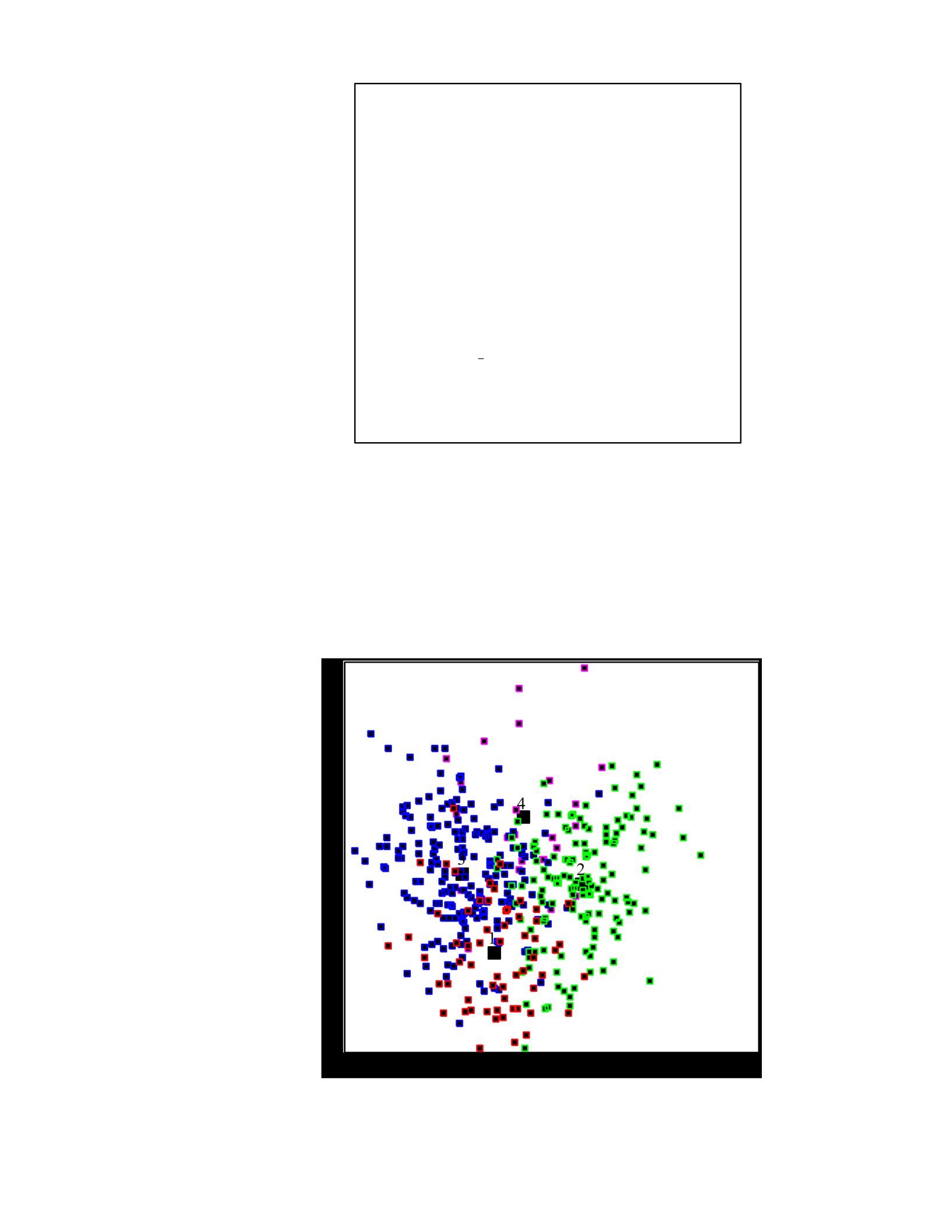
Function 1

Figure 29. A scatter plot of the first two canonical functions for a 19th and 20th century U.S. White

and Black males, morphometroscopic data, axes condensed. Group centroids are marked with a

black dot and are as follows: 19WM = 19th century White males, 19BM = 19th century Black

males, 20WM = 20th century White males, 20BM = 20th century Black males.

3210-1-2

-2

19WM

19BM

BM20

Function 1

Figure 30. A scatter plot of the first two canonical functions for a 19th and 20th century U.S. White

and Black samples, morphometroscopic data. Group centroids are marked with a black square

and are as follows: 1 = 19th century Whites, sexes pooled, 2 = 19th century Blacks, sexes pooled, 3

= 20th century Whites, sexes pooled, 4 = 20th century Blacks, sexes pooled.

Function 1

Figure 31. A scatter plot of the first two canonical functions for a 19th and 20th century U.S. White

and Black samples, morphometroscopic data, axes condensed. Group centroids are marked with

a black dot and are as follows: 19W = 19th century Whites, sexes pooled, 19B = 19th century

Blacks, sexes pooled, 20W = 20th century Whites, sexes pooled, 20B = 20th century Blacks, sexes

pooled.

the first function, as was the case with the morphometric and morphoscopic data models

presented in Chapter 3 (Tables 32 and 33). In these analyses, strong positive scores are

associated with MLT, ARS, and GNI and lesser so with PREI (pooled sexes) and TML23

(males only). Moderate negative scores are associated with XDA (pooled sexes) and

XDA, GOG, GAF (males only). Examination of the mean measures associated with

these variables (Appendix 1) indicates that nearly all mean variable scores are increasing

(or, in the case of GNI for 20th century Black males, staying nearly the same) – thus the

mandible is getting longer and taller in the chin area, wider for the ramus, and more

complex or everted for the ascending ramus. Meanwhile, the width of the palate is

decreasing slightly, as seen in the mean measurements for XDA, and the width of the

gonial region also is decreasing, as evidenced by lower mean values of GOG and GAF

for the 20th century samples.

The results presented in this chapter show that the combination of morphometric and

morphoscopic data, a morphometroscopic data set, can be used to determine population

affinity as well as distinguish between the sexes. Only four of the 28 analyses in this

chapter showed a decrease in the accuracy rates when the morphometroscopic data sets

were used as compared with the morphometric data alone. In each case, the drop in

accuracy was less than 1%. In every analysis, the morphometroscopic data were superior

to the morphoscopic data only models. Generally, the morphometroscopic models

improved over morphometric data sets by approximately 3% and they were over 17%

more accurate than the morphoscopic models. The greatest increases over the

morphometric models were in analyses that contained U.S. Black samples, indicating that

there is a morphoscopic variable strongly tied to the biological affinity of these samples.

Table 32. Structure matrix for the 19th and 20th century U.S. White and Black samples (males),

morphometroscopic data.

Variable Function 1 Function 2 Function 3

WRB 0.477 0.266 0.282

MLT 0.463 0.459 -0.090

PREI 0.410 0.294 0.133

SC -0.289 0.157 -0.107

MAN -0.217 0.188 0.201

XRH -0.197 0.117 0.034

ARS -0.045 0.394 -0.002

GNI 0.331 0.392 -0.015

HML 0.281 0.009 0.413

TLM23 -0.223 0.301 0.325

GOG 0.024 -0.143 -0.283

*Variables not used in this analysis are not shown.

Table 33. Structure matrix for the 19th and 20th century U.S. White and Black samples (sexes

pooled), morphometroscopic data.

Variable Function 1 Function 2 Function 3

PREI 0.449 0.316 -0.279

WRB 0.419 0.262 0.103

SC -0.335 0.127 0.250

MAN -0.223 0.195 -0.185

HML 0.173 0.029 0.082

ARS -0.007 0.395 -0.021

TLM23 -0.232 0.260 0.074

GOG -0.079 -0.186 0.603

XRH -0.257 0.051 0.458

MLT 0.373 0.418 0.426

XDA 0.183 -0.319 0.416

GNI 0.213 0.346 0.385

*Variables not used in this analysis are not shown.

Chapter 5

Discussion

The primary goal of this study was to test the hypothesis that mandibular metrics and

morphology can be used to accurately determine population affinity. Several researchers

have argued that the mandible is a poor skeletal element with which to determine the

biological affinity of an unknown specimen; thus a more concise determination of the

efficacy of mandibular metrics and morphology to the stated problem is needed. As noted

in Chapters 1 and 2, the world is not composed of just Black and White populations,

particularly in forensic situations. Therefore, a more holistic approach was undertaken

and a diverse world-wide selection of samples was applied to this topic. In this study,

three major analytical approaches to the question were used – a morphometric, a

morphoscopic, and a combination of both metrics and morphology – a

morphometroscopic technique. A byproduct of this research was finding that the sex of

an unknown mandible also can be determined using the same three methods. This final

chapter is divided into several sections: first, the results are discussed, second, potential

sources of error are examined, third, a ―big-picture‖ outlook is addressed for these data,

and finally, some forward looking thoughts are presented.

Study Results

Morphometric Data

The next portion of the study focused on the ability of the continuous variables to

adequately determine the sex and the biological affinity of a mandible. Throughout

Chapter 3, the morphometric data largely performed as expected in analyses focused on

sex determination. Indeed, the morphometric variables discriminated between males and

females with accuracy rates equal to or better than those rates published by Giles (1964).

Furthermore, the mandibular morphometric data performed well when compared to

cranial morphometric variables, slightly outperforming facial measurements and

performing equivocally with up to seven vault measurements. This demonstrates that

mandibular morphometric data should not, out of hand, be considered as inferior to

cranial metric data, and that the mandibular morphometric data have a value-added

capacity in sex determination of the human skeleton. In addition to these results, it needs

to be noted that a sex bias in misclassification rates for the morphometric data are present,

similar to that experienced by cranial metric data, when smaller sized individuals are

present in the analyses (e.g. Spradley et al. 2008). The misclassification rates are highest

in the Nubian, Arikara, and Guatemalan population samples, but do not appear to be as

problematic for the U.S. White and Black and the remaining samples. When an analysis

of all samples exclusive of the Nubians, Arikara, and Guatemalan samples (time pooled

U.S. Whites and Blacks) is conducted, the misclassification rates are nearly equal at 15%

males classified as females and 16% females classified as males. Within the population

samples, it appears that most misclassification rates are between 10 and 15%, regardless

of sex, though nearly half of the Cambodian sample females classified as males. The

consumer of this data should be aware of the issue when using the larger discriminant

functions to sex an unknown mandible.

The morphometric variables were used to differentiate between the various population

samples to determine the biological affinity of a specimen. For the total comparison (17

samples), the morphometric variables accuracy rate was 41.4%, or about

7.1 times more accurate than chance alone. This is very good; for a point of comparison,

a 17 group analysis using cranial vault measurements in FORDISC 3.0 (Jantz and Ousley

2005) was conducted, and it yielded an accuracy rate of 56.7% (nine times chance).

When facial measurements were employed, the accuracy rates declined somewhat to

42.4% (seven times chance). It is apparent that the mandibular morphometric data are

slightly underperforming the accuracy rates achieved by cranial vault morphometric

analyses, though they are nearly equivalent to facial measurements, for population

samples of similar size.

In two group comparisons, the morphometric data performed very well, with accuracy

rates ranging from 70% to 96%, depending on the samples and whether the sexes were

pooled. Indeed, in analyses of closely associated groups, e.g. Arikara and Hohokam or

Vietnamese and Chinese, the accuracy rates were approximately 80% on average. In

larger comparisons (3-6 groups), the accuracy rates declined, but the chance of a correct

classification still remained above three times chance, on average. These results hold

mostly true regardless of the type of analysis undertaken, e.g. closely related groups, and

groups through time. The findings presented throughout Chapter 3 show that

discriminant functions based on mandibular morphometrics can be used as a good tool for

assessing the biological affinity of an unknown individual.

Morphoscopic Data

At the outset of this study, a concern of using the morphoscopic (ordinal) data in a

statistical procedure designed for continuous data was that these data violated the

assumptions of the modeling procedure. Therefore, how the ordinal data performed in

these analyses needed to be evaluated. The model performance using ordinal data should

not be judged in terms of the model significance (F-values) due to the stated violated

assumptions. Rather, the appropriate measure of a model’s performance was its

crossvalidated accuracy rate, or how often and how well the model could accurately

predict the sex or biological affinity of an unknown mandible using a leave-one-out

analysis.

The performance results were stated in Chapters 3 and 4, and deserve reviewing here.

For models judging the sex of an unknown mandible, the accuracy rates were greater

than chance for most samples (range 63.5% to 80.5%), although in several comparisons,

the morphological variables could not distinguish between the sexes (Cambodian and

Arikara samples). In general, the ordinal data were hampered by small sample sizes, and

the overall accuracy rates were not nearly as high as models utilizing metric data.

Overall, while sex determination can be accomplished with the morphoscopic data, this

procedure should probably only be undertaken in cases that have a relatively high

accuracy rate (e.g. U. S. Black groups).

When the ordinal data were used to construct models evaluating the biological affinity

of an unknown individual, the accuracy rates increased. In analyses focusing on large

groups, with the sexes analyzed separately, the accuracy rates were at least double that of

chance alone, but with the sexes pooled, the accuracy rates increased to three times

chance alone. The same pattern was observed in analyses focusing on forensically

interesting groups, closely related groups, and groups through time. Two group

comparisons often yielded accuracy rates in the mid 60 percents to the low 80 percents,

and larger comparisons were two to three times chance alone. These analyses show that

the ordinal data can be used to categorize the biological ancestry an unknown mandible

with a moderately good degree of accuracy.

Concerning the analyses focused on closely related groups, the morphoscopic models

had accuracy rates that were 14% worse than the metric analyses, with a range of 2.9%

better to 25.9% worse. Most models, particularly those evaluating more than two groups,

produced results only slightly better than chance. These findings directly contrast with

the higher accuracy rates achieved with the morphological data in analyses of more

widely separated groups (in time or space); this implies that the mandibular morphology

is a better discriminator of very diverse or broad groups rather than geographically

neighboring or related groups.

Another method to determine the morphoscopic variables models’ viability is the data

distributions for the discriminant functions. For this evaluation, the ordinal data were

compared against the morphometric data distributions to determine if models were

differentiating the samples using similar criteria, or if the morphoscopic and

morphometric data were in fact measuring different components of human variation. The

generated scatter plots of the first two canonical components of both data sets were

examined visually for the same sample analyses. In each instance presented in Chapter 3,

the sample distributions and sample centroids were arranged in similar fashions, and in

each instance, the same groups clustered together or were nearly equally separate from

each other. Further, each canonical function was measuring the same underlying

biological variation, e.g. sex, population, or time. These findings indicate that the ordinal

variables have the same substantive ramifications as do the continuous variables. A

byproduct of this analysis is that it is shown now that the morphometric and

morphoscopic data can be effectively combined into a single, morphometroscopic

analysis.

Morphometroscopic Data

While Chapter 3 of this dissertation concentrated on the use of morphoscopic and

morphometric variables independently to determine the sex and biological affinity of an

unknown mandible, Chapter 4 focused on the combination of these variables in

morphometroscopic models. Because analysis of the ordinal data determined that it could

effectively discriminate between the population samples in the same fashion as the

continuous variables, troublesome issues were not foreseen by joining the data sets

together. Rather the question of the accuracy of the morphometroscopic models was the

primary focus of Chapter 4, principally contrasting the mandibular data sets

independently.

Three common themes were apparent in the models throughout Chapter 4. First,

while the generated discriminant functions typically contained both morphometric and

morphoscopic variables, the variable ratio was approximately 3:1 in favor of

morphometric variables for the sex determination functions; on a percentage basis, more

morphometric variables entered into functions for biological affinity than did

morphoscopic variables. Second, in very few morphometroscopic models did the

accuracy rate decline over the best performing model of either morphometric or

morphoscopic origin. In the study models, when the accuracy rates declined, it was

always less than one percent. This finding shows that morphometroscopic models are

superior to those using only one type of variable independently. Third, when analyses

using U.S. Black population samples were undertaken, there was a dramatic accuracy

increase over analyses that utilized morphometric variables only. Conversely, the

accuracy increase was not as dramatic over the morphoscopic variables only analyses, as

compared to analyses that did not contain U.S. Black samples. This finding indicates that

there is a morphoscopic variable tied to the biological ancestry of U.S. Black samples. To

a lesser extent, this finding was also found in analyses utilizing the prehistoric Nubian

sample. When the structure matrices are examined, the PREI variable was the highest

contributing morphoscopic variable in the analyses for U.S. Black samples. This finding

fits well with the earlier work by Angel and Kelley (1990), who indicated that posterior

ramus edge inversion is a particularly racially sensitive trait.

In the sex determination functions, the morphometroscopic models produced accuracy

rates nearly always in excess of 85%, and oftentimes reaching into the low 90 percents.

The lowest accuracy rate in this study was for the Cambodian sample, at 83.1%, which is

likely due to the low number of females in that sample. It is likely that the inclusion of

the Cambodian sample in the ―all samples‖ analysis generated that function’s somewhat

low accuracy rate (85.1%). When misclassification rates are examined, the expected sex

bias was present in the data, particularly for the more gracile or smaller population

samples. But the inclusion of the morphoscopic variables actually helped reduce the bias,

and for the ―all populations‖ analysis, the Nubian and Guatemalan samples decreased

their misclassification rates, while the Arikara sample stayed approximately the same (as

compared to a morphometric function only).

Examination of the variables entering into the functions essentially showed the

expected trend – males are larger than females in both size and expression of traits.

Males are inclined towards a more square or bilobate chin shape, particularly in the U.S.

White samples. Another interesting note is that the 20th century U.S. White and 19th

century U.S. Black males appear to be more predisposed to a partial or complete rocker

jaw shape as compared to the females. This is contrary to the incidence rates of the

rocker jaw noted by Snow (1974) and Schendel et al. (1980), where the females are

clearly more predisposed to this mandibular form than males, albeit these studies only

focused on Polynesian populations.

Turning to biological affinity, examination of the morphometroscopic models’

accuracy rates for the ―all groups analyses‖ shows marked improvements over

morphoscopic data only analyses and moderate improvement in accuracy over the

morphometric only models. For the all groups by sex analysis, the morphometroscopic

model (49.8% accuracy) improved 7% over the morphometric only model and a striking

29.3% over the morphoscopic model. When compared with the same

FORDISC 3.0 analysis presented above, the morphometroscopic model was more

accurate than the facial variables and nearly as accurate as the vault variables. When a

different FORDISC 3.0 analysis of 15 craniofacial measurements was conducted using 17

populations, its accuracy rate varied between 66% and 71%; this demonstrates that

though the mandibular morphometroscopic approach does not perform as well as an

equivalent analysis using the craniofacial skeleton, it still produces results superior to a

mandibular morphoscopic or morphometric only approach, and is likely equal or superior

to limited craniofacial analyses. Thus this method would prove particularly helpful when

only partial or incomplete crania are present for analysis.

When the morphometroscopic approach is used in analyses focusing on forensically

interesting groups and closely related groups, it nearly always outperforms a

morphometric only analysis, and consistently outperformed the morphoscopic analyses.

In only a select few analyses did the morphometroscopic approach fail to achieve the

same accuracy rates as the morphometric models did – in these instances, the inclusion of

admixed populations (e.g. Hispanics) was the norm. The largest increases over

morphometric only models occurred when U.S. Black samples were part of the analysis.

As noted before, this is likely due to the addition of morphoscopic variables that are very

sensitive among those populations.

The morphometroscopic data were employed in several analyses to discriminate

between samples that were closely related in time, e.g. U.S. 19th and 20th century White

and Black males and the same samples with sexes pooled. In these two particular

analyses, the samples very effectively separated along time components, as well as

biological affinity components (see Figures 18 and 19, Chapter 4). The accuracy rates for

the four sample comparisons are in the 60 percents; the odds of a correct assignment of an

unknown mandible were at least three times chance alone. The percent correct represents

a substantial increase over the morphoscopic data when used independent of the

morphometric data and equal or minor increase in accuracy over models using the

morphometric data only.

From the presented study results, it is clear that the morphometroscopic data typically

are superior to either morphometric or morphoscopic data used independently. That said,

both the morphometric and morphoscopic data sets can be used separately, if the data are

not available (or collected), for any given mandible. Specific portions of the mandible

were not tested for their given discriminating power, e.g. the horizontal ramus only, the

ascending ramus only (but see below for two examples). If data for partial and

incomplete mandibles are collected, the data could still be used to classify the unknown

mandible. This type of analysis will be possible when custom discriminant functions are

generated, a planned extension of this research that should be available to investigators in

the future (also see below).

It is patently obvious that as the number of samples increase for any analysis (sex

determination or biological affinity), so do the number of variables entering into the

models. While some variables, e.g. GOG, CDL, GAF, ARS for biological affinity and

many morphoscopic variables for sex determination, do not frequently enter into certain

models, not a single variable was excluded consistently throughout the study. This

indicates that all study variables are important to a model, in a given instance. Each

variable may contain important biological information regarding the ancestry of human

populations or for the sex determination of an unknown individual. Ultimately, future

skeletal analyses should collect the data for all of these variables as part of routine

casework.

Sources of Error

Any study should recognize potential sources of error and take actions to reduce the

errors. Two main areas for error have been identified in this dissertation and methods to

reduce or to evaluate the potential error are discussed. The recognized sources of error

are from missing data (see Chapter 2 for the discussion of missing data) and intra- and

inter-observer error.

Intra and Inter-observer Error

Throughout the data collection process, both the morphometric and morphoscopic

data were gathered twice in order to evaluate intra-observer error. Twenty-four

individuals from the Nubian skeletal sample were measured twice using eight

measurements (GNI, HML, CDL, GOG, WRB, XRH, MAN, and MLT). The second set

of measurements was collected approximately two years after the first set. Paired

samples t-tests were used to evaluate whether or not there were significant amounts of

measurement error between the two data sets. One measurement, MLT, was significantly

different between the two measuring episodes (p = .003). It was consistently measured

larger the first time over the second. Several possibilities exist for the discrepancy in the

measurements. First, due to a relatively small sample size, significance testing is heavily

influenced by even minor discrepancies. The median difference in all values for this

measurement was -0.333 mm, which was, in fact, the largest discrepancy of any of the

measurements. But merely changing two measurement values by one mm each produces

a non-significant result for the paired-samples t-tests. Second, two different

mandibulometers were used, and error may have occurred due to the different types of

equipment. Third, this could be a real source of error. A fourth source could be recording

errors. A larger sample size may be warranted for future exploration, though typically,

deviation of around 3% between observers is expected for most skeletal measurements

(Adams and Byrd 2002).

For the morphoscopic data, the CIL Vietnamese sample was scored on two different

occasions, approximately one year apart. Again, 24 mandibles were re-scored, using all

six study variables. Wilcoxon signed ranks tests and Pearson’s R correlations were

conducted on these data. The resulting Pearson’s R correlations all were greater than

0.97 except for CS, which was 0.87, indicating strong concordance in the two data sets.

No significant difference was found between the data using Wilcoxon signed ranks tests.

The overall dispersion of the data does indicate some slight discrepancies – both the GAF

and PREI variables had three differences between scoring sessions. In each case, the

differences were one category different, and for GAF, were unidirectional (GAF was

consistently scored larger the second time). While no significant difference was detected

using this sample, additional testing on a larger sample may be warranted.

Data for a structured inter-observer analysis were not collected for this study. While

differences between investigators can pose a challenge to scientific data, the data

collection procedures used in this study do not depart heavily from standard procedures

used in daily case work or data collection and should not depart significantly from the

published inter-observer error rates for skeletal elements (e.g. Adams and Byrd 2002;

Jantz et al. 1995). For the morphometric data, two new measurements XDA and TML23,

were devised for this study. The measurement locations are clearly defined and

photographs are given in Appendix 1 for correct measuring procedures. Given the

simplicity of these measurements and the detailed definitions, it is not expected that much

inter-observer error would be encountered. The morphoscopic data may prove to be

slightly more difficult to score consistently between investigators. Physical

anthropologists are used to scoring the morphoscopic features of various human bones,

and generally speaking, do quite well between themselves (c.f. Berg in press; Iscan and

Loth 1986a, 1986b; Kimmerle et al., in press; Sutherland and Suchey 1991). For the

specific morphoscopic features used here, most are well-known to the anthropology

community and distributions of their prevalence in various samples have been

documented (Angel and Kelley 1990; Rhine 1990; Hauser and De Stefano 1989).

Overall, little intra-observer error was found in this study, though the sample size was

small. Some detected error could be due to small sample sizes, recording errors, or

equipment differences. Other error, while not significant, could lead to erroneous

conclusions, on a case by case basis. Inter-observer error was not specifically tested,

though given the precautions taken in this study, its effects should be mitigated or reduced

with the judicious and deliberate application of the supplied definitions and exemplars.

Additional testing of the data collection procedures, particularly for interobserver error

testing, may be warranted.

The Big Picture

Human variation is rich and diverse, and the need for forensic classification models to

mirror human diversity is paramount. Many applied forensic anthropology techniques

and methods are restricted in the scope of the variation characterized, often due to the

limited accessibility of collections, money, and time. This study has attempted to

incorporate a more diverse world population sample than is typically found in the older

literature, or in current forensic anthropological undertakings. Twelve world groups

composed of seventeen samples are represented in this study, from Asia to the Americas,

and from prehistory to modern times. While the sample sizes are arguably low for certain

groups, the overall study sample is robust and well-balanced. Due to this diversity in the

research design, the study results have meaningful ramifications for forensic

anthropology.

Perhaps one of the most important points to be made, which has been consistently

alluded to throughout this study, is that single collections of human remains are not

suitable for creating methods to identify unknown individuals from. Indeed, a more

holistic and broad-based approach is needed. It is not acceptable to force the phenotypic

characters of modern humans into models based on humans hundreds of years old (e.g.

using the Terry collection to characterize current U.S. White and Black individuals).

This study among others has shown significant changes in these groups, such that they

can be separated out from each other using appropriate models. Instead, these data

should be gathered but labeled appropriately for hypothesis testing, and other collections

should be used for modern U.S. samples (e.g. the William Bass collection), modern

Asians (e.g. Killing Fields collections, assorted Medical Examiner collections), and

modern Hispanics (e.g. Medical Examiner collections).

Prior to this study, only certain morphoscopic traits of the mandible could be used

easily to make statements regarding biological affinity (Angel and Kelley 1990; Rhine

1990), frequently regarding those of U.S. White or Black descent. Likewise, mandibular

morphometrics were readily available only for U.S. White or Black populations through

FORDISC 2.0 (Ousley and Jantz 1996). Methods examining the sexual dimorphism of

the mandible were likewise narrow (e.g. Bass 2005; Buikstra and Ubelaker 1994; Ousley

and Jantz 1996). The methods using morphology of the mandible did not include error or

accuracy rates, though cross-validated error rates were available in FORDISC 2.0

(Ousley and Jantz 1996). In the latest release of FORDISC 3.0 (Jantz and Ousley 2005),

morphometric analysis of the mandible does include two additional populations,

Guatemalans and Japanese, though the number of metric variables is limited. A sex-only

function is not possible with the program now, due to the stated problems with the sex

bias found for more gracile or smaller populations.

This research provides additional data and especially formulae to evaluate the sex and

ancestry of an unknown individual though the use of morphometric, morphoscopic, or

morphometroscopic data acquired from the mandible. This study has imparted immediate

access to formulae that can ascertain the sex of an unknown individual

without knowing the ancestry, or if a priori information is available, the method can be

specialized to just a few groups. Any determination of sex made by an ―anthropologist

on the ground‖ has the added surety of established accuracy rates, as well as potential

error rates. The user must be aware of the sex bias in the data though (and cases where it

is small), and interpretation of the data is left in the users hands. More importantly, the

study has demonstrated that all three methods can be used to deduce the ancestry of an

unknown mandible. A morphometroscopic approach typically works the best; a

morphometric approach frequently succeeds with greater accuracy than a morphoscopic

approach, though a morphoscopic analysis does surprisingly well, particularly when U.S.

Black samples are included. Indeed, with accuracy rates greater than 90% for some two

population sample comparisons or eight times chance for the largest analyses, the results

of this study run contrary to the opinions expressed by Humphrey and co-workers (1999).

While Humphrey et al. (1999) believe that mandibular plasticity renders this element

impractical for identifying relationships among human populations, it is perhaps this

same plasticity that imparts a useful quality for forensic and ancestral determination

applications.

The determination of ancestral phenotypic expressions of genetic traits in the human

skeletal system is a daunting task. As it becomes more acceptable for individuals to pair

and procreate with members of different background, the overall human phenotype will

become more centrist and less polarized toward particular expressions. Conversely, if

social mating patterns were to shift toward a closed group pattern, phenotypes should

become more polarized. In today’s increasingly multicultural environment, admixture is

present, and appears to be increasing (see Chapter 1). Three possible outcomes of this

genetic mixing are foreseen: one, the skeletal expressions of admixture should, in theory,

decrease the overall efficacy of discriminant formulae among groups as the admixture

percentage climbs; two, discriminant models that contain relatively ―pure‖ samples

should have better accuracy rates than models containing admixed populations,

particularly if the admixed sample contains genetic components from the comparative

group; and three, samples from the same population but from different eras (e.g. 18th, 19th,

or 20th century samples from U.S. Whites or Blacks) may differentiate statistically

(secular change and admixture).

The first scenario may be relatively difficult to empirically test with these data, as the

amount of admixture in U.S. populations is not necessarily all that great, yet. Second, the

number of clearly documented admixed individuals is very low in skeletal collections

throughout the U.S. One possible evaluation method for this scenario would be to

determine the accuracy rates for discriminant functions comparing 19th century White and

Black samples versus 20th century samples, with the assumption that genetic admixture is

increasing within the samples through time. For 19th century individuals, the accuracy

rate is 79.2%, and the analysis contained approximately equal sample sizes (U.S. White =

55, U.S. Black = 70). The accuracy rate declined 2.4% for the 20th century analysis to

76.8%, but the sample size is relatively low in the U.S. Black sample (n = 27) compared

to the U.S. White sample (n = 163). While the hypothesis of declining accuracy rates

does appear to hold true in this example, it might just be a function of the small sample

size of 20th century U.S. Black individuals. A larger sample size and several types of

samples through time are necessary to determine if this hypothesis will hold.

Evidence for the second scenario, that is analyses containing more ―pure‖ samples

having higher accuracy rates than admixed samples, is present in the data. For example,

the accuracy rate for the function examining Arikara and Cambodian samples was 95.4%

accurate (relatively ―pure‖ samples) while an analysis of the 20th century U.S. White

male and Hispanic male samples only produced an accuracy rate of 71.7% (―pure‖ and

admixed samples, respectively). This shows that difficulties are likely to be encountered

when admixed populations are used in comparisons; on the other hand, the accuracy rate

will depend on the samples compared and whether or not the ―admixed‖ sample contains

genetic components of the comparative sample. For example, a relatively admixed

sample, the 20th century U.S. Black male sample was compared with the Guatemalan

male sample and the ensuing accuracy rate was excellent (94.8%), even though both

samples contain admixture, but they do not likely contain ―shared‖ genetic components

(i.e. the Guatemalan samples potentially contain very few African genes, but likely do

contain high genetic components from multiple Native American groups and minor

amounts of European influence). But when the same U.S. population was compared with

Hispanic males, the accuracy rate dropped precipitously (80.0%). Since the Hispanic

sample is heavily influenced by Native American, European, and African genes and the

U.S. Black sample is likely influenced by European genes, the ensuing accuracy rate of

the comparison is expected – much lower than comparisons of samples lacking

significantly shared genetic components.

The third possibility also was documented in this study, secular change. In Chapters 3

and 4, U.S. White and Black male samples do separate from each other ancestrally, and

along time components. Changes in the shape and size of the mandible are apparent from

the data. Both the U.S. White and Black 20th century samples are gaining size in the chin,

width of the ramus, bicondylar width, and in the mandibular angle as compared with their

19th century counterparts. The mandible is also becoming more complex in shape, with

more mandibular tori, larger expressions of posterior ramus edge inversion, a more

complex chin, and the ascending rami are increasing to a uniform width. Both of these

groups are following a similar trajectory in the noted secular changes.

Forces identified as playing a role in secular change for height and length of limb

bones include nutrition and disease load (Jantz and Jantz 1999; Price et al. 1987). Hosts

of other factors such as income distribution, temperature, a genetically determined

ceiling, birth weight, and genetic variation rather than plasticity also have been correlated

to secular changes in stature and cranio-metric variation (Alberman et al. 1991; Jantz and

Jantz 1999; Price et al. 1987; Wescott and Jantz 2005). Wescott and Jantz (2005) have

argued that a parallel course of secular change seen in American Whites and Blacks

cranial measurements, combined with their failure to converge on a common type, is

evidence of genetic variation rather than plasticity in the cranium. Jantz and Jantz (1999)

have argued that secular changes in stature are likely not the simple formula of height =

intake-demand, and that factors influencing early childhood development play a role in

secular change. Other regions of the body such as the cranium also have shown secular

change; nutritional status has been suggested as a possible causal agent of these changes.

Environmentally-determined constraints, such as brain growth, biochemical or

developmental constraints have been proposed as causal agents as well (Cameron et al.

1990). The positive secular trend seen in the current data may be due to any of these

factors, or as hinted at earlier, may be in part due to admixture.

Interestingly, in the comparisons that assess primarily for a time component, the

centroid for the 20th century U.S. Black sample is moving toward the U.S. White

centroids (19th or 20th century) along function 1 (see Figures 16-17, 29 and 31). When

compared against each other, the distance moved on function 1 for 20th century birth years

is over double that for U.S. Black than U.S. White samples. The 20th century U.S. Black

centroid moved a distance of +1.533 units from the 19th century U. S. Black centroid,

while a distance of +0.682 units was moved along function 1 for the 20th century U. S.

White sample. The 20th century U.S. Black sample’s centroid is -0.644 units from the 19th

century U.S. White centroid. The movement of the U.S. Black sample toward the U.S.

White sample centroids suggests that not only are factors such as health and nutrition

playing a role in the phenotypic expressions present in U.S. Black samples, but also that

genetic admixture may be closing the gap between them. Given that 20th century U.S.

Black samples contain nearly a 20% admixture of U.S. White genetic data

(Parra et al. 1998, 2001) and that 20th century U.S. White samples have little admixture

(Shriver et al. 2003), it is conceivable that the mandibular morphometroscopic,

morphometric, and morphoscopic scatter plots are graphically detailing the effect of

admixture on the 20th century U.S. Black samples.

Looking Forward

This study has opened the door to many other topics that can and should be addressed

in upcoming research. While this study focused on 17 world samples, additional samples

should be added to the database to better characterize unknown individuals. Specifically,

the low sample sizes in the U.S. 20th century Black males and females, as well as the 19th

century White females need attention. Other population samples can use additional data

collection. This study would also greatly benefit from a test of the scoring and measuring

methods between and among investigators. In order to be effectively used in a court of

law, error rates need to be firmly understood (see Daubert v. Merrell Dow

Pharmaceuticals No. 92-102 509 US 579, 1993). This can be accomplished through the

measuring of several samples by multiple investigators. While the study did produce

error rates for the author, additional error rates should be determined for members of the

physical anthropology community.

Another avenue for exploration is found in the contribution of individual variables to

the discriminant functions and the frequency in which certain variables are present in the

models. The statistical contribution of each variable to a given function or series of

functions could shed light on overarching questions of human variation. Given the shear

number of functions possible with these data, this research avenue was determined to be

outside the scope of this study.

In this study, the statistical package was allowed to choose which variables entered

into the functions based on the amount of information they contained for the question at

hand. No specific attempt was made to limit the functions to specific portions of the

mandible, such as the ramus or corpus, within the main study parameters. Ultimately, the

accuracy rate of any one given function will be a result of the data for a particular set of

variables; since incomplete data sets are the norm in forensic and physical anthropology,

a need for ―custom‖ discriminant functions is apparent. Two short examples can be put

forward here, one using the chin area only, the second using an ascending ramus only.

For the chin area, five variables are used to determine the sex or biological affinity of the

unknown individual – GNI, TML, HML, MT, and CS. A custom discriminant function

for ―sex only‖ with 12 samples has an accuracy rate of 73% (all variables entering), and

30% accuracy rate for biological affinity (about 4 times chance alone). If the

morphoscopic variables are not included, the accuracy rate for sex drops to 70% and

biological affinity drops to 22%. For the ascending ramus example, six variables are

obtained – TLM23, XRH, WRB, GAF, ARS, PREI. Again, a custom discriminant

function produced an accuracy rate of 81% for ―sex only‖ function (all but ARS were

present in the function) and a 27% accuracy rate for biological affinity (3.2 times chance

alone). (Both analyses accuracy rates drop approximately 3% and 5% respectively if the

morphoscopic variables are not included.)

The tool to accomplish the goal of having the ability to produce custom discriminant

functions for whichever variables are present could be found in the form of an updated

version of FORDISC, or a new computer program that is web-accessible. The data from

this project will be made available to the authors of FORDISC, so that a separate module

can be created. Since this process may take several years to complete, these data are

made freely available by contacting the author.

This study has ultimately shown that both mandibular morphometric and

morphoscopic data, particularly when used in a morphometroscopic analysis, can

effectively classify the sex of an unknown mandible (used appropriately) and the

biological affinity of a mandible of known and unknown sex. The formulae for some

sexual dimorphism discriminant functions are presented in this dissertation;

comprehensive models for biological affinity were not made available, due to their length

and complexity. Overall, this dissertation has achieved its goal – to provide another tool

in the forensic anthropologist’s kit for the determination of the biological affinity and sex

of an unknown individual.

Introduction Biological affinity studies or geographic

Students also viewed