

Database Systems
 lord mots
Database Design - 2nd Edition
Database Design - 2nd Edition
Adrienne Watt
Nelson Eng
Unless otherwise noted within this book, this book is released under a Creative Commons Attribution 3.0 Unported License also known
as a CC-BY license. This means you are free to copy, redistribute, modify or adapt this book. Under this license, anyone who redistributes
or modifies this textbook, in whole or in part, can do so for free providing they properly attribute the book.
Additionally, if you redistribute this textbook, in whole or in part, in either a print or digital format, then you must retain on every physical
and/or electronic page the following attribution:
Download this book for free at http://open.bccampus.ca
Cover image: Spiral Stairs In Milano old building downtown by Michele Ursino used under a CC-BY-SA 2.0 license .
Database Design - 2nd Edition by Adrienne Watt and Nelson Eng is licensed under a Creative Commons Attribution 4.0 International
License, except where otherwise noted
Contents
Preface vi
About the Book vii
Acknowledgements viii
Chapter 1 Before the Advent of Database Systems
Adrienne Watt
1
Chapter 2 Fundamental Concepts
Adrienne Watt & Nelson Eng
6
Chapter 3 Characteristics and Benefits of a Database
Adrienne Watt
9
Chapter 4 Types of Data Models
Adrienne Watt & Nelson Eng
13
Chapter 5 Data Modelling
Adrienne Watt
15
Chapter 6 Classification of Database Management Systems
Adrienne Watt
21
Chapter 7 The Relational Data Model
Adrienne Watt
24
Chapter 8 The Entity Relationship Data Model
Adrienne Watt
29
Chapter 9 Integrity Rules and Constraints
Adrienne Watt & Nelson Eng
44
Chapter 10 ER Modelling
Adrienne Watt
55
Chapter 11 Functional Dependencies
Adrienne Watt
61
Chapter 12 Normalization
Adrienne Watt
66
Chapter 13 Database Development Process
Adrienne Watt
74
Chapter 14 Database Users
Adrienne Watt
82
Chapter 15 SQL Structured Query Language
Adrienne Watt & Nelson Eng
83
Chapter 16 SQL Data Manipulation Language
Adrienne Watt & Nelson Eng
94
Appendix A University Registration Data Model Example 113
Appendix B Sample ERD Exercises 117
iv
Appendix C SQL Lab with Solution 120
About the Authors 127
v
Preface
The primary purpose of this text is to provide an open source textbook that covers most introductory database courses.
The material in the textbook was obtained from a variety of sources. All the sources are found in at the end of each
chapter. I expect, with time, the book will grow with more information and more examples.
I welcome any feedback that would improve the book. If you would like to add a section to the book, please let me know.
Adrienne Watt
vi •
vi
About the Book
Database Design – 2nd Edition is a remix and adaptation, based on Adrienne Watt’s book, Database Design. Works that are
part of the remix for this book are listed at the end of each chapter. For information about what was changed in this
adaptation, refer to the Copyright statement at the bottom of the home page.
This adaptation is a part of the B.C. Open Textbook project.
In October 2012, the B.C. Ministry of Advanced Education announced its support for the creation of open textbooks
for the 40 highest-enrolled first and second year subject areas in the province’s public post-secondary system.
Open textbooks are open educational resources (OER); they are instructional resources created and shared in ways
so that more people have access to them. This is a different model than traditionally copyrighted materials. OER are
defined as “teaching, learning, and research resources that reside in the public domain or have been released under
an intellectual property license that permits their free use and re-purposing by others (Hewlett Foundation).
Our open textbooks are openly licensed using a Creative Commons license, and are offered in various e-book formats
free of charge, or as printed books that are available at cost.
For more information about this project, please contact [email protected].
vii
Acknowledgements
Adrienne Watt
This book has been a wonderful experience in the world of open textbooks. It’s amazing to see how much information
is available to be shared. I would like to thank Nguyen Kim Anh of OpenStax College, for her contribution of database
models and the relational design sections. I would also like to thank Dr. Gordon Russell for the section on normaliza-
tion. His database resources were wonderful. Open Learning University in the UK provided me with a great ERD exam-
ple. In addition, Tom Jewet provided some invaluable UML contributions.
I would also like to thank my many students over the years and a special instructor, Mitra Ramkay (BCIT). He is fondly
remembered for the mentoring he provided when I first started teaching relational databases 25 years ago. Another
person instrumental in getting me started in creating an open textbook is Terrie MacAloney. She was encouraging and
taught me think outside the box.
A special thanks goes to my family for the constant love and support I received throughout this project.
Nelson Eng
I would like to thank the many people who helped in this edition including my students at Douglas College and my col-
league Ms. Adrienne Watt.
We would like to particularly thank Lauri Aesoph at BCcampus for her perseverance and hard work while editing the
book. She did an amazing job.
viii •
viii
Chapter 1 Before the Advent of Database Systems Adrienne Watt
The way in which computers manage data has come a long way over the last few decades. Today’s users take for granted
the many benefits found in a database system. However, it wasn’t that long ago that computers relied on a much less
elegant and costly approach to data management called the file-based system.
File-based System
One way to keep information on a computer is to store it in permanent files. A company system has a number of appli-
cation programs; each of them is designed to manipulate data files. These application programs have been written at
the request of the users in the organization. New applications are added to the system as the need arises. The system just
described is called the file-based system.
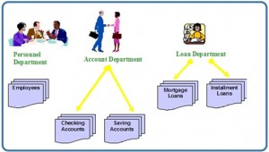
Consider a traditional banking system that uses the file-based system to manage the organization’s data shown in Figure
1.1. As we can see, there are different departments in the bank. Each has its own applications that manage and manip-
ulate different data files. For banking systems, the programs may be used to debit or credit an account, find the balance
of an account, add a new mortgage loan and generate monthly statements.
Figure 1.1. Example of a file-based system used by banks to manage
data.
Disadvantages of the file-based approach
Using the file-based system to keep organizational information has a number of disadvantages. Listed below are five
examples.
Data redundancy
Often, within an organization, files and applications are created by different programmers from various departments
over long periods of time. This can lead to data redundancy, a situation that occurs in a database when a field needs to be
updated in more than one table. This practice can lead to several problems such as:
• Inconsistency in data format
• The same information being kept in several different places (files)
1
• Data inconsistency, a situation where various copies of the same data are conflicting, wastes storage space and
duplicates effort
Data isolation
Data isolation is a property that determines when and how changes made by one operation become visible to other con-
current users and systems. This issue occurs in a concurrency situation. This is a problem because:
• It is difficult for new applications to retrieve the appropriate data, which might be stored in various files.
Integrity problems
Problems with data integrity is another disadvantage of using a file-based system. It refers to the maintenance and assur-
ance that the data in a database are correct and consistent. Factors to consider when addressing this issue are:
• Data values must satisfy certain consistency constraints that are specified in the application programs.
• It is difficult to make changes to the application programs in order to enforce new constraints.
Security problems
Security can be a problem with a file-based approach because:
• There are constraints regarding accessing privileges.
• Application requirements are added to the system in an ad-hoc manner so it is difficult to enforce
constraints.
Concurrency access
Concurrency is the ability of the database to allow multiple users access to the same record without adversely affecting
transaction processing. A file-based system must manage, or prevent, concurrency by the application programs. Typi-
cally, in a file-based system, when an application opens a file, that file is locked. This means that no one else has access
to the file at the same time.
In database systems, concurrency is managed thus allowing multiple users access to the same record. This is an impor-
tant difference between database and file-based systems.
Database Approach
The difficulties that arise from using the file-based system have prompted the development of a new approach in man-
aging large amounts of organizational information called the database approach.
Databases and database technology play an important role in most areas where computers are used, including business,
education and medicine. To understand the fundamentals of database systems, we will start by introducing some basic
concepts in this area.
2 •
THIS TEXTBOOK IS AVAILABLE FOR FREE AT OPEN.BCCAMPUS.CA
Role of databases in business
Everybody uses a database in some way, even if it is just to store information about their friends and family. That data
might be written down or stored in a computer by using a word-processing program or it could be saved in a spread-
sheet. However, the best way to store data is by using database management software. This is a powerful software tool that
allows you to store, manipulate and retrieve data in a variety of different ways.
Most companies keep track of customer information by storing it in a database. This data may include customers,
employees, products, orders or anything else that assists the business with its operations.
The meaning of data
Data are factual information such as measurements or statistics about objects and concepts. We use data for discussions
or as part of a calculation. Data can be a person, a place, an event, an action or any one of a number of things. A single
fact is an element of data, or a data element.
If data are information and information is what we are in the business of working with, you can start to see where you
might be storing it. Data can be stored in:
• Filing cabinets
• Spreadsheets
• Folders
• Ledgers
• Lists
• Piles of papers on your desk
All of these items store information, and so too does a database. Because of the mechanical nature of databases, they
have terrific power to manage and process the information they hold. This can make the information they house much
more useful for your work.
With this understanding of data, we can start to see how a tool with the capacity to store a collection of data and organize
it, conduct a rapid search, retrieve and process, might make a difference to how we can use data. This book and the
chapters that follow are all about managing information.
Key Terms
concurrency: the ability of the database to allow multiple users access to the same record without adversely
affecting transaction processing
data element: a single fact or piece of information
data inconsistency: a situation where various copies of the same data are conflicting
data isolation: a property that determines when and how changes made by one operation become visible to oth-
er concurrent users and systems
data integrity: refers to the maintenance and assurance that the data in a database are correct and consistent
CHAPTER 1 BEFORE THE ADVENT OF DATABASE SYSTEMS • 3
THIS TEXTBOOK IS AVAILABLE FOR FREE AT OPEN.BCCAMPUS.CA
data redundancy: a situation that occurs in a database when a field needs to be updated in more than one table
database approach: allows the management of large amounts of organizational information
database management software: a powerful software tool that allows you to store, manipulate and retrieve
data in a variety of ways
file-based system: an application program designed to manipulate data files
Exercises
1. Discuss each of the following terms:
1.1 data
1.2 field
1.3 record
1.4 file
2. What is data redundancy?
3. Discuss the disadvantages of file-based systems.
4. Explain the difference between data and information.
5. Use Figure 1.2 (below) to answer the following questions.
5.1 In the table, how many records does the file contain?
5.2 How many fields are there per record?
5.3 What problem would you encounter if you wanted to produce a listing by city?
5.4 How would you solve this problem by altering the file structure?
Figure 1.2. Table for exercise #5, by A. Watt.
Attribution
This chapter of Database Design (including its images, unless otherwise noted) is a derivative copy of Database System
Concepts by Nguyen Kim Anh licensed under Creative Commons Attribution License 3.0 license
The following material was written by Adrienne Watt:
1. Introduction
4 •
THIS TEXTBOOK IS AVAILABLE FOR FREE AT OPEN.BCCAMPUS.CA
2. Key Terms
3. Exercises
CHAPTER 1 BEFORE THE ADVENT OF DATABASE SYSTEMS • 5
THIS TEXTBOOK IS AVAILABLE FOR FREE AT OPEN.BCCAMPUS.CA
Chapter 2 Fundamental Concepts Adrienne Watt & Nelson Eng
What Is a Database?
A database is a shared collection of related data used to support the activities of a particular organization. A database can
be viewed as a repository of data that is defined once and then accessed by various users as shown in Figure 2.1.
Figure 2.1. A database is a repository of data.
Database Properties
A database has the following properties:
• It is a representation of some aspect of the real world or a collection of data elements (facts) representing real-
world information.
• A database is logical, coherent and internally consistent.
• A database is designed, built and populated with data for a specific purpose.
• Each data item is stored in a field.
• A combination of fields makes up a table. For example, each field in an employee table contains data about an
individual employee.
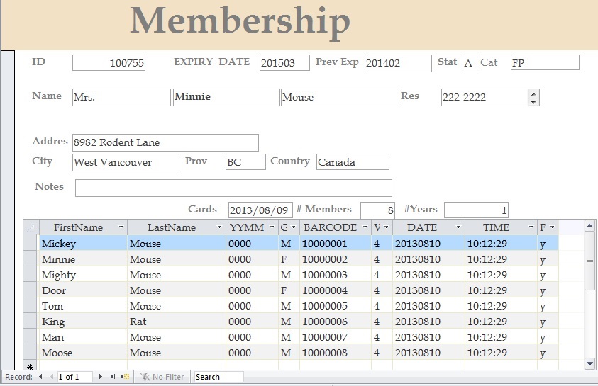
A database can contain many tables. For example, a membership system may contain an address table and an individual
member table as shown in Figure 2.2. Members of Science World are individuals, group homes, businesses and corpora-
tions who have an active membership to Science World. Memberships can be purchased for a one- or two-year period,
and then renewed for another one- or two-year period.
In Figure 2.2, Minnie Mouse renewed the family membership with Science World. Everyone with membership
ID#100755 lives at 8932 Rodent Lane. The individual members are Mickey Mouse, Minnie Mouse, Mighty Mouse,
Door Mouse, Tom Mouse, King Rat, Man Mouse and Moose Mouse.
6
Figure 2.2. Membership system at Science World by N. Eng.
Database Management System
A database management system (DBMS) is a collection of programs that enables users to create and maintain databases
and control all access to them. The primary goal of a DBMS is to provide an environment that is both convenient and
efficient for users to retrieve and store information.
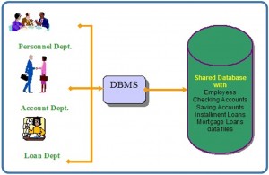
With the database approach, we can have the traditional banking system as shown in Figure 2.3. In this bank example, a
DBMS is used by the Personnel Department, the Account Department and the Loan Department to access the shared
corporate database.
Figure 2.3. A bank database management system (DBMS).
Key Terms
data elements: facts that represent real-world information
CHAPTER 2 FUNDAMENTAL CONCEPTS • 7
THIS TEXTBOOK IS AVAILABLE FOR FREE AT OPEN.BCCAMPUS.CA
database: a shared collection of related data used to support the activities of a particular organization
database management system (DBMS): a collection of programs that enables users to create and maintain
databases and control all access to them
table: a combination of fields
Exercises
1. What is a database management system (DBMS)?
2. What are the properties of a DBMS?
3. Provide three examples of a real-world database (e.g., the library contains a database of books).
Attribution
This chapter of Database Design (including images, except as otherwise noted) is a derivative copy of Database System
Concepts by Nguyen Kim Anh licensed under Creative Commons Attribution License 3.0 license
The following material was written by Nelson Eng:
1. Example under Database Properties
2. Key Terms
The following material was written by Adrienne Watt:
1. Exercises
8 •
THIS TEXTBOOK IS AVAILABLE FOR FREE AT OPEN.BCCAMPUS.CA
Chapter 3 Characteristics and Benefits of a Database Adrienne Watt
Managing information means taking care of it so that it works for us and is useful for the tasks we perform. By using a
DBMS, the information we collect and add to its database is no longer subject to accidental disorganization. It becomes
more accessible and integrated with the rest of our work. Managing information using a database allows us to become
strategic users of the data we have.
We often need to access and re-sort data for various uses. These may include:
• Creating mailing lists
• Writing management reports
• Generating lists of selected news stories
• Identifying various client needs
The processing power of a database allows it to manipulate the data it houses, so it can:
• Sort
• Match
• Link
• Aggregate
• Skip fields
• Calculate
• Arrange
Because of the versatility of databases, we find them powering all sorts of projects. A database can be linked to:
• A website that is capturing registered users
• A client-tracking application for social service organizations
• A medical record system for a health care facility
• Your personal address book in your email client
• A collection of word-processed documents
• A system that issues airline reservations
Characteristics and Benefits of a Database
There are a number of characteristics that distinguish the database approach from the file-based system or approach.
This chapter describes the benefits (and features) of the database system.
Self-describing nature of a database system
A database system is referred to as self-describing because it not only contains the database itself, but also metadata which
defines and describes the data and relationships between tables in the database. This information is used by the DBMS
9
software or database users if needed. This separation of data and information about the data makes a database system
totally different from the traditional file-based system in which the data definition is part of the application programs.
Insulation between program and data
In the file-based system, the structure of the data files is defined in the application programs so if a user wants to change
the structure of a file, all the programs that access that file might need to be changed as well.
On the other hand, in the database approach, the data structure is stored in the system catalogue and not in the pro-
grams. Therefore, one change is all that is needed to change the structure of a file. This insulation between the programs
and data is also called program-data independence.
Support for multiple views of data
A database supports multiple views of data. A view is a subset of the database, which is defined and dedicated for partic-
ular users of the system. Multiple users in the system might have different views of the system. Each view might contain
only the data of interest to a user or group of users.
Sharing of data and multiuser system
Current database systems are designed for multiple users. That is, they allow many users to access the same database at
the same time. This access is achieved through features called concurrency control strategies. These strategies ensure that
the data accessed are always correct and that data integrity is maintained.
The design of modern multiuser database systems is a great improvement from those in the past which restricted usage
to one person at a time.
Control of data redundancy
In the database approach, ideally, each data item is stored in only one place in the database. In some cases, data redun-
dancy still exists to improve system performance, but such redundancy is controlled by application programming and
kept to minimum by introducing as little redudancy as possible when designing the database.
Data sharing
The integration of all the data, for an organization, within a database system has many advantages. First, it allows for
data sharing among employees and others who have access to the system. Second, it gives users the ability to generate
more information from a given amount of data than would be possible without the integration.
Enforcement of integrity constraints
Database management systems must provide the ability to define and enforce certain constraints to ensure that users
enter valid information and maintain data integrity. A database constraint is a restriction or rule that dictates what can be
entered or edited in a table such as a postal code using a certain format or adding a valid city in the City field.
There are many types of database constraints. Data type, for example, determines the sort of data permitted in a field, for
example numbers only. Data uniqueness such as the primary key ensures that no duplicates are entered. Constraints can
be simple (field based) or complex (programming).
10 •
THIS TEXTBOOK IS AVAILABLE FOR FREE AT OPEN.BCCAMPUS.CA
Restriction of unauthorized access
Not all users of a database system will have the same accessing privileges. For example, one user might have read-only
access (i.e., the ability to read a file but not make changes), while another might have read and write privileges, which is the
ability to both read and modify a file. For this reason, a database management system should provide a security subsys-
tem to create and control different types of user accounts and restrict unauthorized access.
Data independence
Another advantage of a database management system is how it allows for data independence. In other words, the
system data descriptions or data describing data (metadata) are separated from the application programs. This is possible
because changes to the data structure are handled by the database management system and are not embedded in the
program itself.
Transaction processing
A database management system must include concurrency control subsystems. This feature ensures that data remains
consistent and valid during transaction processing even if several users update the same information.
Provision for multiple views of data
By its very nature, a DBMS permits many users to have access to its database either individually or simultaneously. It is
not important for users to be aware of how and where the data they access is stored
Backup and recovery facilities
Backup and recovery are methods that allow you to protect your data from loss. The database system provides a sepa-
rate process, from that of a network backup, for backing up and recovering data. If a hard drive fails and the database
stored on the hard drive is not accessible, the only way to recover the database is from a backup.
If a computer system fails in the middle of a complex update process, the recovery subsystem is responsible for making
sure that the database is restored to its original state. These are two more benefits of a database management system.
Key Terms
concurrency control strategies: features of a database that allow several users access to the same data item at
the same time
data type: determines the sort of data permitted in a field, for example numbers only
data uniqueness: ensures that no duplicates are entered
database constraint: a restriction that determines what is allowed to be entered or edited in a table
metadata: defines and describes the data and relationships between tables in the database
read and write privileges: the ability to both read and modify a file
CHAPTER 3 CHARACTERISTICS AND BENEFITS OF A DATABASE • 11
THIS TEXTBOOK IS AVAILABLE FOR FREE AT OPEN.BCCAMPUS.CA
read-onlyaccess: the ability to read a file but not make changes
self-describing: a database system is referred to as self-describing because it not only contains the database
itself, but also metadata which defines and describes the data and relationships between tables in the database
view: a subset of the database
Exercises
1. How is a DBMS distinguished from a file-based system?
2. What is data independence and why is it important?
3. What is the purpose of managing information?
4. Discuss the uses of databases in a business environment.
5. What is metadata?
Attribution
This chapter of Database Design is a derivative copy of Database System Concepts by Nguyen Kim Anh licensed
under Creative Commons Attribution License 3.0 license
The following material was written by Adrienne Watt:
1. Introduction
2. Key Terms
3. Exercises
12 •
THIS TEXTBOOK IS AVAILABLE FOR FREE AT OPEN.BCCAMPUS.CA
Chapter 4 Types of Data Models Adrienne Watt & Nelson Eng
High-level Conceptual Data Models
High-level conceptual data models provide concepts for presenting data in ways that are close to the way people perceive
data. A typical example is the entity relationship model, which uses main concepts like entities, attributes and relation-
ships. An entity represents a real-world object such as an employee or a project. The entity has attributes that represent
properties such as an employee’s name, address and birthdate. A relationship represents an association among entities;
for example, an employee works on many projects. A relationship exists between the employee and each project.
Record-based Logical Data Models
Record-based logical data models provide concepts users can understand but are not too far from the way data is stored
in the computer. Three well-known data models of this type are relational data models, network data models and hier-
archical data models.
• The relational model represents data asrelations, or tables. For example, in the membership system at Science
World, each membership has many members (see Figure 2.2 in Chapter 2). The membership identifier, expiry
date and address information are fields in the membership. The members are individuals such as Mickey,
Minnie, Mighty, Door, Tom, King, Man and Moose. Each record is said to be an instance of the membership
table.
• The network model represents data as record types. This model also represents a limited type of one to many
relationship called a set type, as shown in Figure 4.1.
Figure 4.1. Network model diagram.
• The hierarchical model represents data as a hierarchical tree structure. Each branch of the hierarchy represents
a number of related records. Figure 4.2 shows this schema in hierarchical model notation.
13
Figure 4.2. Hierarchical model diagram.
Key Terms
hierarchical model: represents data as a hierarchical tree structure
instance: a record within a table
network model: represents data as record types
relation: another term for table
relational model: represents data as relations or tables
set type: a limited type of one to many relationship
Exercises
1. What is a data model?
2. What is a high-level conceptual data model?
3. What is an entity? An attribute? A relationship?
4. List and briefly describe the common record-based logical data models.
Attribution
This chapter of Database Design is a derivative copy of Database System Concepts by Nguyen Kim Anh licensed
under Creative Commons Attribution License 3.0 license
The following material was written by Adrienne Watt:
1. Key Terms
2. Exercises
14 •
THIS TEXTBOOK IS AVAILABLE FOR FREE AT OPEN.BCCAMPUS.CA
Chapter 5 Data Modelling Adrienne Watt
Data modelling is the first step in the process of database design. This step is sometimes considered to be a high-level and
abstract design phase, also referred to as conceptual design. The aim of this phase is to describe:
• The data contained in the database (e.g., entities: students, lecturers, courses, subjects)
• The relationships between data items (e.g., students are supervised by lecturers; lecturers teach courses)
• The constraints on data (e.g., student number has exactly eight digits; a subject has four or six units of credit
only)
In the second step, the data items, the relationships and the constraints are all expressed using the concepts provided
by the high-level data model. Because these concmepts do not include the implementation details, the result of the data
modelling process is a (semi) formal representation of the database structure. This result is quite easy to understand so
it is used as reference to make sure that all the user’s requirements are met.
The third step is database design. During this step, we might have two sub-steps: one called database logical design, which
defines a database in a data model of a specific DBMS, and another called database physical design, which defines the
internal database storage structure, file organization or indexing techniques. These two sub-steps are database imple-
mentation and operations/user interfaces building steps.
In the database design phases, data are represented using a certain data model. The data model is a collection of concepts
or notations for describing data, data relationships, data semantics and data constraints. Most data models also include
a set of basic operations for manipulating data in the database.
Degrees of Data Abstraction
In this section we will look at the database design process in terms of specificity. Just as any design starts at a high level
and proceeds to an ever-increasing level of detail, so does database design. For example, when building a home, you start
with how many bedrooms and bathrooms the home will have, whether it will be on one level or multiple levels, etc. The
next step is to get an architect to design the home from a more structured perspective. This level gets more detailed with
respect to actual room sizes, how the home will be wired, where the plumbing fixtures will be placed, etc. The last step is
to hire a contractor to build the home. That’s looking at the design from a high level of abstraction to an increasing level
of detail.
The database design is very much like that. It starts with users identifying the business rules; then the database designers
and analysts create the database design; and then the database administrator implements the design using a DBMS.
The following subsections summarize the models in order of decreasing level of abstraction.
External models
• Represent the user’s view of the database
• Contain multiple different external views
• Are closely related to the real world as perceived by each user
15
Conceptual models
• Provide flexible data-structuring capabilities
• Present a “community view”: the logical structure of the entire database
• Contain data stored in the database
• Show relationships among data including:
Constraints
Semantic information (e.g., business rules)
Security and integrity information
• Consider a database as a collection of entities (objects) of various kinds
• Are the basis for identification and high-level description of main data objects; they avoid details
• Are database independent regardless of the database you will be using
Internal models
The three best-known models of this kind are the relational data model, the network data model and the hierarchical
data model. These internal models:
• Consider a database as a collection of fixed-size records
• Are closer to the physical level or file structure
• Are a representation of the database as seen by the DBMS.
• Require the designer to match the conceptual model’s characteristics and constraints to those of the selected
implementation model
• Involve mapping the entities in the conceptual model to the tables in the relational model
Physical models
• Are the physical representation of the database
• Have the lowest level of abstractions
• Are how the data is stored; they deal with
Run-time performance
Storage utilization and compression
File organization and access methods
Data encryption
• Are the physical level – managed by the operating system (OS)
• Provide concepts that describe the details of how data are stored in the computer’s memory
Data Abstraction Layer
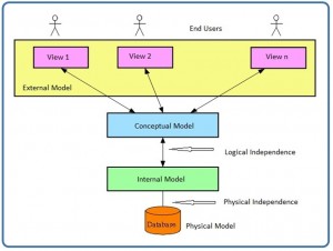
In a pictorial view, you can see how the different models work together. Let’s look at this from the highest level, the
external model.
The external model is the end user’s view of the data. Typically a database is an enterprise system that serves the needs
of multiple departments. However, one department is not interested in seeing other departments’ data (e.g., the human
16 •
THIS TEXTBOOK IS AVAILABLE FOR FREE AT OPEN.BCCAMPUS.CA
resources (HR) department does not care to view the sales department’s data). Therefore, one user view will differ from
another.
The external model requires that the designer subdivide a set of requirements and constraints into functional modules
that can be examined within the framework of their external models (e.g., human resources versus sales).
As a data designer, you need to understand all the data so that you can build an enterprise-wide database. Based on the
needs of various departments, the conceptual model is the first model created.
At this stage, the conceptual model is independent of both software and hardware. It does not depend on the DBMS
software used to implement the model. It does not depend on the hardware used in the implementation of the model.
Changes in either hardware or DBMS software have no effect on the database design at the conceptual level.
Once a DBMS is selected, you can then implement it. This is the internal model. Here you create all the tables, con-
straints, keys, rules, etc. This is often referred to as the logical design.
The physical model is simply the way the data is stored on disk. Each database vendor has its own way of storing the
data.
Figure 5.1. Data abstraction layers.
Schemas
A schema is an overall description of a database, and it is usually represented by the entity relationship diagram (ERD).
There are many subschemas that represent external models and thus display external views of the data. Below is a list of
items to consider during the design process of a database.
• External schemas: there are multiple
• Multiple subschemas: these display multiple external views of the data
• Conceptual schema: there is only one. This schema includes data items, relationships and constraints, all
represented in an ERD.
• Physical schema: there is only one
CHAPTER 5 DATA MODELLING • 17
THIS TEXTBOOK IS AVAILABLE FOR FREE AT OPEN.BCCAMPUS.CA
Logical and Physical Data Independence
Data independence refers to the immunity of user applications to changes made in the definition and organization of data.
Data abstractions expose only those items that are important or pertinent to the user. Complexity is hidden from the
database user.
Data independence and operation independence together form the feature of data abstraction. There are two types of
data independence: logical and physical.
Logical data independence
A logical schema is a conceptual design of the database done on paper or a whiteboard, much like architectural drawings
for a house. The ability to change the logical schema, without changing the external schema or user view, is called logical
data independence. For example, the addition or removal of new entities, attributes or relationships to this conceptual
schema should be possible without having to change existing external schemas or rewrite existing application programs.
In other words, changes to the logical schema (e.g., alterations to the structure of the database like adding a column or
other tables) should not affect the function of the application (external views).
Physical data independence
Physical data independence refers to the immunity of the internal model to changes in the physical model. The logical
schema stays unchanged even though changes are made to file organization or storage structures, storage devices or
indexing strategy.
Physical data independence deals with hiding the details of the storage structure from user applications. The applica-
tions should not be involved with these issues, since there is no difference in the operation carried out against the data.
Key Terms
conceptual model: the logical structure of the entire database
conceptual schema: another term for logical schema
data independence: the immunity of user applications to changes made in the definition and organization of
data
data model: a collection of concepts or notations for describing data, data relationships, data semantics and data
constraints
data modelling: the first step in the process of database design
database logical design: defines a database in a data model of a specific database management system
database physical design: defines the internal database storage structure, file organization or indexing tech-
niques
18 •
THIS TEXTBOOK IS AVAILABLE FOR FREE AT OPEN.BCCAMPUS.CA
entity relationship diagram (ERD): a data model describing the database showing tables, attributes and rela-
tionships
external model: represents the user’s view of the database
external schema: user view
internal model: a representation of the database as seen by the DBMS
logical data independence: the ability to change the logical schema without changing the external schema
logical design: where you create all the tables, constraints, keys, rules, etc.
logical schema: a conceptual design of the database done on paper or a whiteboard, much like architectural
drawings for a house
operating system (OS): manages the physical level of the physical model
physical data independence: the immunity of the internal model to changes in the physical model
physical model: the physical representation of the database
schema: an overall description of a database
Exercises
1. Describe the purpose of a conceptual design.
2. How is a conceptual design different from a logical design?
3. What is an external model?
4. What is a conceptual model?
5. What is an internal model?
6. What is a physical model?
7. Which model does the database administrator work with?
8. Which model does the end user work with?
9. What is logical data independence?
10. What is physical data independence?
Also see Appendix A: University Registration Data Model Example
Attribution
This chapter of Database Design is a derivative copy of Database System Concepts by Nguyen Kim Anh licensed
under Creative Commons Attribution License 3.0 license
CHAPTER 5 DATA MODELLING • 19
THIS TEXTBOOK IS AVAILABLE FOR FREE AT OPEN.BCCAMPUS.CA
The following material was written by Adrienne Watt:
• Some or all of the introduction, degrees of data abstraction, data abstraction layer
• Key Terms
• Exercises
20 •
THIS TEXTBOOK IS AVAILABLE FOR FREE AT OPEN.BCCAMPUS.CA
Chapter 6 Classification of Database Management Systems Adrienne Watt
Database management systems can be classified based on several criteria, such as the data model, user numbers and
database distribution, all described below.
Classification Based on Data Model
The most popular data model in use today is the relational data model. Well-known DBMSs like Oracle, MS SQL Server,
DB2 and MySQL support this model. Other traditional models, such as hierarchical data models and network data mod-
els, are still used in industry mainly on mainframe platforms. However, they are not commonly used due to their com-
plexity. These are all referred to as traditional models because they preceded the relational model.
In recent years, the newer object-oriented data models were introduced. This model is a database management system in
which information is represented in the form of objects as used in object-oriented programming. Object-oriented data-
bases are different from relational databases, which are table-oriented. Object-oriented database management systems
(OODBMS) combine database capabilities with object-oriented programming language capabilities.
The object-oriented models have not caught on as expected so are not in widespread use. Some examples of object-ori-
ented DBMSs are O2, ObjectStore and Jasmine.
Classification Based on User Numbers
A DBMS can be classification based on the number of users it supports. It can be a single-user database system, which
supports one user at a time, or a multiuser database system, which supports multiple users concurrently.
Classification Based on Database Distribution
There are four main distribution systems for database systems and these, in turn, can be used to classify the DBMS.
Centralized systems
With a centralized database system, the DBMS and database are stored at a single site that is used by several other systems
too. This is illustrated in Figure 6.1.
In the early 1980s, many Canadian libraries used the GEAC 8000 to convert their manual card catalogues to machine-
readable centralized catalogue systems. Each book catalogue had a barcode field similar to those on supermarket prod-
ucts.
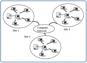
Distributed database system
In a distributed database system, the actual database and the DBMS software are distributed from various sites that are
connected by a computer network, as shown in Figure 6.2.
21
Figure 6.1. Example of a centralized database system.
Figure 6.2. Example of a distributed database system.
Homogeneous distributed database systems
Homogeneous distributed database systems use the same DBMS software from multiple sites. Data exchange between these
various sites can be handled easily. For example, library information systems by the same vendor, such as Geac Comput-
er Corporation, use the same DBMS software which allows easy data exchange between the various Geac library sites.
Heterogeneous distributed database systems
In a heterogeneous distributed database system, different sites might use different DBMS software, but there is additional
common software to support data exchange between these sites. For example, the various library database systems use
the same machine-readable cataloguing (MARC) format to support library record data exchange.
Key Terms
centralized database system: the DBMS and database are stored at a single site that is used by several other
systems too
22 •
THIS TEXTBOOK IS AVAILABLE FOR FREE AT OPEN.BCCAMPUS.CA
distributed database system: the actual database and the DBMS software are distributed from various sites that
are connected by a computer network
heterogeneous distributed database system: different sites might use different DBMS software, but there is
additional common software to support data exchange between these sites
homogeneous distributed database systems: use the same DBMS software at multiple sites
multiuser database system: a database management system which supports multiple users concurrently
object-oriented data model: a database management system in which information is represented in the form
of objects as used in object-oriented programming
single-user database system: a database management system which supports one user at a time
traditional models: data models that preceded the relational model
Exercises
1. Provide three examples of the most popular relational databases used.
2. What is the difference between centralized and distributed database systems?
3. What is the difference between homogenous distributed database systems and heterogeneous
distributed database systems?
Attribution
This chapter of Database Design (including images, except as otherwise noted) is a derivative copy of Database System
Concepts by Nguyen Kim Anh licensed under Creative Commons Attribution License 3.0 license
The following material was written by Adrienne Watt:
1. Key Terms
2. Exercises
CHAPTER 6 CLASSIFICATION OF DATABASE MANAGEMENT SYSTEMS • 23
THIS TEXTBOOK IS AVAILABLE FOR FREE AT OPEN.BCCAMPUS.CA
Chapter 7 The Relational Data Model Adrienne Watt
The relational data model was introduced by C. F. Codd in 1970. Currently, it is the most widely used data model.
The relational model has provided the basis for:
• Research on the theory of data/relationship/constraint
• Numerous database design methodologies
• The standard database access language called structured query language (SQL)
• Almost all modern commercial database management systems
The relational data model describes the world as “a collection of inter-related relations (or tables).”
Fundamental Concepts in the Relational Data Model
Relation
A relation, also known as a table or file, is a subset of the Cartesian product of a list of domains characterized by a
name. And within a table, each row represents a group of related data values. A row, or record, is also known as a tuple.
The columns in a table is a field and is also referred to as an attribute. You can also think of it this way: an attribute is
used to define the record and a record contains a set of attributes.
The steps below outline the logic between a relation and its domains.
1. Given n domains are denoted by D1, D2, … Dn
2. And r is a relation defined on these domains
3. Then r ? D1×D2×…×Dn
Table
A database is composed of multiple tables and each table holds the data. Figure 7.1 shows a database that contains three
tables.
Column
A database stores pieces of information or facts in an organized way. Understanding how to use and get the most out of
databases requires us to understand that method of organization.
The principal storage units are called columns or fields or attributes. These house the basic components of data into
which your content can be broken down. When deciding which fields to create, you need to think generically about your
information, for example, drawing out the common components of the information that you will store in the database
and avoiding the specifics that distinguish one item from another.
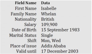
Look at the example of an ID card in Figure 7.2 to see the relationship between fields and their data.
24
Figure 7.1. Database with three tables.
Figure 7.2. Example of an ID card by A. Watt.
Domain
A domain is the original sets of atomic values used to model data. By atomic value, we mean that each value in the domain
is indivisible as far as the relational model is concerned. For example:
• The domain of Marital Status has a set of possibilities: Married, Single, Divorced.
• The domain of Shift has the set of all possible days: {Mon, Tue, Wed…}.
• The domain of Salary is the set of all floating-point numbers greater than 0 and less than 200,000.
• The domain of First Name is the set of character strings that represents names of people.
In summary, a domain is a set of acceptable values that a column is allowed to contain. This is based on various proper-
ties and the data type for the column. We will discuss data types in another chapter.
Records
Just as the content of any one document or item needs to be broken down into its constituent bits of data for storage
in the fields, the link between them also needs to be available so that they can be reconstituted into their whole form.
Records allow us to do this. Records contain fields that are related, such as a customer or an employee. As noted earlier,
a tuple is another term used for record.
CHAPTER 7 THE RELATIONAL DATA MODEL • 25
THIS TEXTBOOK IS AVAILABLE FOR FREE AT OPEN.BCCAMPUS.CA
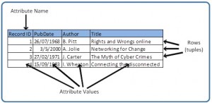
Records and fields form the basis of all databases. A simple table gives us the clearest picture of how records and fields
work together in a database storage project.
Figure 7.3. Example of a simple table by A. Watt.
The simple table example in Figure 7.3 shows us how fields can hold a range of different sorts of data. This one has:
• A Record ID field: this is an ordinal number; its data type is an integer.
• A PubDate field: this is displayed as day/month/year; its data type is date.
• An Author field: this is displayed as Initial. Surname; its data type is text.
• A Title field text: free text can be entered here.
You can command the database to sift through its data and organize it in a particular way. For example, you can request
that a selection of records be limited by date: 1. all before a given date, 2. all after a given date or 3. all between two given
dates. Similarly, you can choose to have records sorted by date. Because the field, or record, containing the data is set up
as a Date field, the database reads the information in the Date field not just as numbers separated by slashes, but rather,
as dates that must be ordered according to a calendar system.
Degree
The degree is the number of attributes in a table. In our example in Figure 7.3, the degree is 4.
Properties of a Table
• A table has a name that is distinct from all other tables in the database.
• There are no duplicate rows; each row is distinct.
• Entries in columns are atomic. The table does not contain repeating groups or multivalued attributes.
• Entries from columns are from the same domain based on their data type including:
number (numeric, integer, float, smallint,…)
character (string)
date
logical (true or false)
• Operations combining different data types are disallowed.
• Each attribute has a distinct name.
• The sequence of columns is insignificant.
• The sequence of rows is insignificant.
26 •
THIS TEXTBOOK IS AVAILABLE FOR FREE AT OPEN.BCCAMPUS.CA
Key Terms
atomic value: each value in the domain is indivisible as far as the relational model is concerned
attribute: principle storage unit in a database
column: see attribute
degree: number of attributes in a table
domain: the original sets of atomic values used to model data; a set of acceptable values that a column is allowed
to contain
field: see attribute
file: see relation
record: contains fields that are related; see tuple
relation: a subset of the Cartesian product of a list of domains characterized by a name; the technical term for
table or file
row: see tuple
structured query language (SQL): the standard database access language
table: see relation
tuple: a technical term for row or record
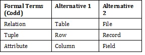
Terminology Key
Several of the terms used in this chapter are synonymous. In addition to the Key Terms above, please refer to
Table 7.1 below. The terms in the Alternative 1 column are most commonly used.
Table 7.1. Terms and their synonyms by A. Watt.
CHAPTER 7 THE RELATIONAL DATA MODEL • 27
THIS TEXTBOOK IS AVAILABLE FOR FREE AT OPEN.BCCAMPUS.CA
Exercises
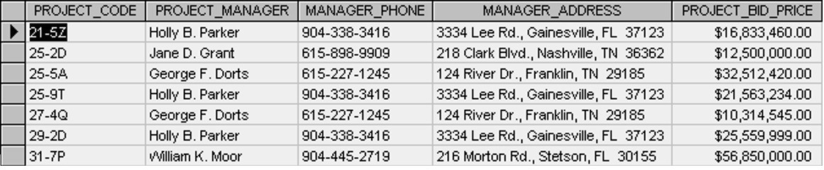
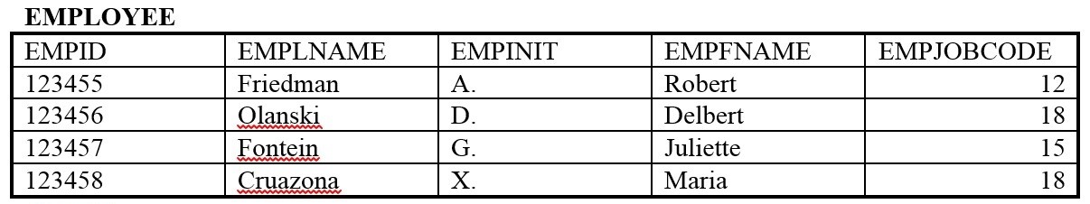
Use Table 7.2 to answer questions 1-4.
1. Using correct terminology, identify and describe all the components in Table 7.2.
2. What is the possible domain for field EmpJobCode?
3. How many records are shown?
4. How many attributes are shown?
5. List the properties of a table.
Table 7.2. Table for exercise questions, by A. Watt.
Attribution
This chapter of Database Design (including images, except as otherwise noted) is a derivative copy of Relational Design
Theory by Nguyen Kim Anh licensed under Creative Commons Attribution License 3.0 license
The following material was written by Adrienne Watt:
1. All or part of the sections on relations, tables, columns and degree
2. Key Terms
3. Exercises
28 •
THIS TEXTBOOK IS AVAILABLE FOR FREE AT OPEN.BCCAMPUS.CA
Chapter 8 The Entity Relationship Data Model Adrienne Watt
The entity relationship (ER) data model has existed for over 35 years. It is well suited to data modelling for use with data-
bases because it is fairly abstract and is easy to discuss and explain. ER models are readily translated to relations. ER
models, also called an ER schema, are represented by ER diagrams.
ER modelling is based on two concepts:
• Entities, defined as tables that hold specific information (data)
• Relationships, defined as the associations or interactions between entities
Here is an example of how these two concepts might be combined in an ER data model: Prof. Ba (entity) teaches (rela-
tionship) the Database Systems course (entity).
For the rest of this chapter, we will use a sample database called the COMPANY database to illustrate the concepts of
the ER model. This database contains information about employees, departments and projects. Important points to note
include:
• There are several departments in the company. Each department has a unique identification, a name, location
of the office and a particular employee who manages the department.
• A department controls a number of projects, each of which has a unique name, a unique number and
a budget.
• Each employee has a name, identification number, address, salary and birthdate. An employee is assigned to
one department but can join in several projects. We need to record the start date of the employee in each
project. We also need to know the direct supervisor of each employee.
• We want to keep track of the dependents for each employee. Each dependent has a name, birthdate and
relationship with the employee.
Entity, Entity Set and Entity Type
An entity is an object in the real world with an independent existence that can be differentiated from other objects. An
entity might be
• An object with physical existence (e.g., a lecturer, a student, a car)
• An object with conceptual existence (e.g., a course, a job, a position)
Entities can be classified based on their strength. An entity is considered weak if its tables are existence dependent.
• That is, it cannot exist without a relationship with another entity
• Its primary key is derived from the primary key of the parent entity
The Spouse table, in the COMPANY database, is a weak entity because its primary key is
dependent on the Employee table. Without a corresponding employee record, the spouse record
would not exist.
29
An entity is considered strong if it can exist apart from all of its related entities.
• Kernels are strong entities.
• A table without a foreign key or a table that contains a foreign key that can contain nulls is a strong entity
Another term to know is entity type which defines a collection of similar entities.
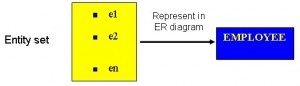
An entity set is a collection of entities of an entity type at a particular point of time. In an entity relationship diagram
(ERD), an entity type is represented by a name in a box. For example, in Figure 8.1, the entity type is EMPLOYEE.
Figure 8.1. ERD with entity type EMPLOYEE.
Existence dependency
An entity’s existence is dependent on the existence of the related entity. It is existence-dependent if it has a mandatory
foreign key (i.e., a foreign key attribute that cannot be null). For example, in the COMPANY database, a Spouse entity is
existence -dependent on the Employee entity.
Kinds of Entities
You should also be familiar with different kinds of entities including independent entities, dependent entities and char-
acteristic entities. These are described below.
Independent entities
Independent entities, also referred to as kernels, are the backbone of the database. They are what other tables are based
on. Kernels have the following characteristics:
• They are the building blocks of a database.
• The primary key may be simple or composite.
• The primary key is not a foreign key.
• They do not depend on another entity for their existence.
If we refer back to our COMPANY database, examples of an independent entity include the Customer table, Employee
table or Product table.
Dependent entities
Dependent entities, also referred to as derived entities, depend on other tables for their meaning. These entities have the
following characteristics:
• Dependent entities are used to connect two kernels together.
30 •
THIS TEXTBOOK IS AVAILABLE FOR FREE AT OPEN.BCCAMPUS.CA
• They are said to be existence dependent on two or more tables.
• Many to many relationships become associative tables with at least two foreign keys.
• They may contain other attributes.
• The foreign key identifies each associated table.
• There are three options for the primary key:
1. Use a composite of foreign keys of associated tables if unique
2. Use a composite of foreign keys and a qualifying column
3. Create a new simple primary key
Characteristic entities
Characteristic entities provide more information about another table. These entities have the following characteristics:
• They represent multivalued attributes.
• They describe other entities.
• They typically have a one to many relationship.
• The foreign key is used to further identify the characterized table.
• Options for primary key are as follows:
1. Use a composite of foreign key plus a qualifying column
2. Create a new simple primary key. In the COMPANY database, these might include:
* Employee (EID, Name, Address, Age, Salary) – EID is the simple primary key.
* EmployeePhone (EID, Phone) – EID is part of a composite primary key. Here, EID is
also a foreign key.
Attributes
Each entity is described by a set of attributes (e.g., Employee = (Name, Address, Birthdate (Age), Salary).
Each attribute has a name, and is associated with an entity and a domain of legal values. However, the information about
attribute domain is not presented on the ERD.
In the entity relationship diagram, shown in Figure 8.2, each attribute is represented by an oval with a name inside.
Figure 8.2. How attributes are represented in an ERD.
CHAPTER 8 THE ENTITY RELATIONSHIP DATA MODEL • 31
THIS TEXTBOOK IS AVAILABLE FOR FREE AT OPEN.BCCAMPUS.CA
Types of Attributes
There are a few types of attributes you need to be familiar with. Some of these are to be left as is, but some need to be
adjusted to facilitate representation in the relational model. This first section will discuss the types of attributes. Later
on we will discuss fixing the attributes to fit correctly into the relational model.
Simple attributes
Simple attributes are those drawn from the atomic value domains; they are also called single-valued attributes. In the COM-
PANY database, an example of this would be: Name = {John} ; Age = {23}
Composite attributes
Composite attributes are those that consist of a hierarchy of attributes. Using our database example, and shown in Figure
8.3, Address may consist of Number, Street and Suburb. So this would be written as → Address = {59 + ‘Meek Street’ +
‘Kingsford’}
Figure 8.3. An example of composite attributes.
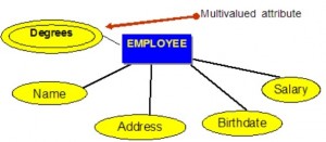
Multivalued attributes
Multivalued attributes are attributes that have a set of values for each entity. An example of a multivalued attribute from
the COMPANY database, as seen in Figure 8.4, are the degrees of an employee: BSc, MIT, PhD.
Figure 8.4. Example of a multivalued attribute.
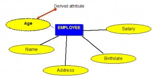
Derived attributes
Derived attributes are attributes that contain values calculated from other attributes. An example of this can be seen in
Figure 8.5. Age can be derived from the attribute Birthdate. In this situation, Birthdate is called a stored attribute, which
is physically saved to the database.
32 •
THIS TEXTBOOK IS AVAILABLE FOR FREE AT OPEN.BCCAMPUS.CA
Figure 8.5. Example of a derived attribute.
Keys
An important constraint on an entity is the key. The key is an attribute or a group of attributes whose values can be used
to uniquely identify an individual entity in an entity set.
Types of Keys
There are several types of keys. These are described below.
Candidate key
A candidate key is a simple or composite key that is unique and minimal. It is unique because no two rows in a table may
have the same value at any time. It is minimal because every column is necessary in order to attain uniqueness.
From our COMPANY database example, if the entity is Employee(EID, First Name, Last Name, SIN, Address, Phone,
BirthDate, Salary, DepartmentID), possible candidate keys are:
• EID, SIN
• First Name and Last Name – assuming there is no one else in the company with the same name
• Last Name and DepartmentID – assuming two people with the same last name don’t work in the same
department
Composite key
A composite key is composed of two or more attributes, but it must be minimal.
Using the example from the candidate key section, possible composite keys are:
• First Name and Last Name – assuming there is no one else in the company with the same name
• Last Name and Department ID – assuming two people with the same last name don’t work in the same
department
CHAPTER 8 THE ENTITY RELATIONSHIP DATA MODEL • 33
THIS TEXTBOOK IS AVAILABLE FOR FREE AT OPEN.BCCAMPUS.CA
Primary key
The primary key is a candidate key that is selected by the database designer to be used as an identifying mechanism for
the whole entity set. It must uniquely identify tuples in a table and not be null. The primary key is indicated in the ER
model by underlining the attribute.
• A candidate key is selected by the designer to uniquely identify tuples in a table. It must not be null.
• A key is chosen by the database designer to be used as an identifying mechanism for the whole entity set.
This is referred to as the primary key. This key is indicated by underlining the attribute in the ER model.
In the following example, EID is the primary key:
Employee(EID, First Name, Last Name, SIN, Address, Phone, BirthDate, Salary, DepartmentID)
Secondary key
A secondary key is an attribute used strictly for retrieval purposes (can be composite), for example: Phone and Last Name.
Alternate key
Alternate keys are all candidate keys not chosen as the primary key.
Foreign key
A foreign key (FK) is an attribute in a table that references the primary key in another table OR it can be null. Both foreign
and primary keys must be of the same data type.
In the COMPANY database example below, DepartmentID is the foreign key:
Employee(EID, First Name, Last Name, SIN, Address, Phone, BirthDate, Salary, DepartmentID)
Nulls
A null is a special symbol, independent of data type, which means either unknown or inapplicable. It does not mean zero
or blank. Features of null include:
• No data entry
• Not permitted in the primary key
• Should be avoided in other attributes
• Can represent
An unknown attribute value
A known, but missing, attribute value
A “not applicable” condition
• Can create problems when functions such as COUNT, AVERAGE and SUM are used
• Can create logical problems when relational tables are linked
34 •
THIS TEXTBOOK IS AVAILABLE FOR FREE AT OPEN.BCCAMPUS.CA
NOTE: The result of a comparison operation is null when either argument is null. The result of an arithmetic operation
is null when either argument is null (except functions that ignore nulls).
Example of how null can be used
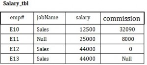
Use the Salary table (Salary_tbl) in Figure 8.6 to follow an example of how null can be used.
Figure 8.6. Salary table for null example, by A. Watt.
To begin, find all employees (emp#) in Sales (under the jobName column) whose salary plus commission are greater than
30,000.
• SELECT emp# FROM Salary_tbl
• WHERE jobName = Sales AND
• (commission + salary) > 30,000 –> E10 and E12
This result does not include E13 because of the null value in the commission column. To ensure that the row with the
null value is included, we need to look at the individual fields. By adding commission and salary for employee E13, the
result will be a null value. The solution is shown below.
• SELECT emp# FROM Salary_tbl
• WHERE jobName = Sales AND
• (commission > 30000 OR
• salary > 30000 OR
• (commission + salary) > 30,000 –>E10 and E12 and E13
Relationships
Relationships are the glue that holds the tables together. They are used to connect related information between tables.
Relationship strength is based on how the primary key of a related entity is defined. A weak, or non-identifying, rela-
tionship exists if the primary key of the related entity does not contain a primary key component of the parent entity.
Company database examples include:
• Customer(CustID, CustName)
• Order(OrderID, CustID, Date)
A strong, or identifying, relationship exists when the primary key of the related entity contains the primary key compo-
nent of the parent entity. Examples include:
CHAPTER 8 THE ENTITY RELATIONSHIP DATA MODEL • 35
THIS TEXTBOOK IS AVAILABLE FOR FREE AT OPEN.BCCAMPUS.CA
• Course(CrsCode, DeptCode, Description)
• Class(CrsCode, Section, ClassTime…)
Types of Relationships
Below are descriptions of the various types of relationships.
One to many (1:M) relationship
A one to many (1:M) relationship should be the norm in any relational database design and is found in all relational
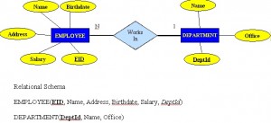
database environments. For example, one department has many employees. Figure 8.7 shows the relationship of one of
these employees to the department.
Figure 8.7. Example of a one to many relationship.
One to one (1:1) relationship
A one to one (1:1) relationship is the relationship of one entity to only one other entity, and vice versa. It should be rare
in any relational database design. In fact, it could indicate that two entities actually belong in the same table.
An example from the COMPANY database is one employee is associated with one spouse, and one spouse is associated
with one employee.
Many to many (M:N) relationships
For a many to many relationship, consider the following points:
• It cannot be implemented as such in the relational model.
• It can be changed into two 1:M relationships.
• It can be implemented by breaking up to produce a set of 1:M relationships.
• It involves the implementation of a composite entity.
• Creates two or more 1:M relationships.
• The composite entity table must contain at least the primary keys of the original tables.
• The linking table contains multiple occurrences of the foreign key values.
• Additional attributes may be assigned as needed.
• It can avoid problems inherent in an M:N relationship by creating a composite entity or bridge entity. For
example, an employee can work on many projects OR a project can have many employees working on it,
depending on the business rules. Or, a student can have many classes and a class can hold many students.
36 •
THIS TEXTBOOK IS AVAILABLE FOR FREE AT OPEN.BCCAMPUS.CA
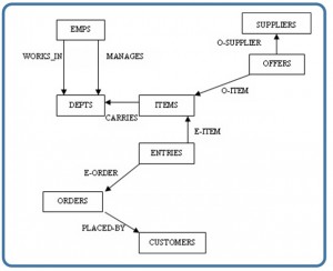
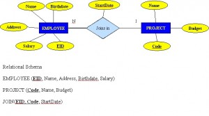
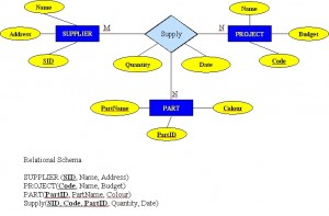
Figure 8.8 shows another another aspect of the M:N relationship where an employee has different start dates for differ-
ent projects. Therefore, we need a JOIN table that contains the EID, Code and StartDate.
Figure 8.8. Example where employee has different start dates for differ-
ent projects.
Example of mapping an M:N binary relationship type
• For each M:N binary relationship, identify two relations.
• A and B represent two entity types participating in R.
• Create a new relation S to represent R.
• S needs to contain the PKs of A and B. These together can be the PK in the S table OR these together with
another simple attribute in the new table R can be the PK.
• The combination of the primary keys (A and B) will make the primary key of S.
Unary relationship (recursive)
A unary relationship, also called recursive, is one in which a relationship exists between occurrences of the same entity set.
In this relationship, the primary and foreign keys are the same, but they represent two entities with different roles. See
Figure 8.9 for an example.
For some entities in a unary relationship, a separate column can be created that refers to the primary key of the same
entity set.
Figure 8.9. Example of a unary relationship.
CHAPTER 8 THE ENTITY RELATIONSHIP DATA MODEL • 37
THIS TEXTBOOK IS AVAILABLE FOR FREE AT OPEN.BCCAMPUS.CA
Ternary Relationships
A ternary relationship is a relationship type that involves many to many relationships between three tables.
Refer to Figure 8.10 for an example of mapping a ternary relationship type. Note n-ary means multiple tables in a rela-
tionship. (Remember, N = many.)
• For each n-ary (> 2) relationship, create a new relation to represent the relationship.
• The primary key of the new relation is a combination of the primary keys of the participating entities that
hold the N (many) side.
• In most cases of an n-ary relationship, all the participating entities hold a many side.
Figure 8.10. Example of a ternary relationship.
Key Terms
alternate key: all candidate keys not chosen as the primary key
candidate key: a simple or composite key that is unique (no two rows in a table may have the same value) and
minimal (every column is necessary)
characteristic entities: entities that provide more information about another table
composite attributes: attributes that consist of a hierarchy of attributes
composite key: composed of two or more attributes, but it must be minimal
dependent entities: these entities depend on other tables for their meaning
derived attributes: attributes that contain values calculated from other attributes
derived entities: see dependent entities
EID: employee identification (ID)
38 •
THIS TEXTBOOK IS AVAILABLE FOR FREE AT OPEN.BCCAMPUS.CA
entity: a thing or object in the real world with an independent existence that can be differentiated from other
objects
entity relationship (ER) data model: also called an ER schema, are represented by ER diagrams. These are well
suited to data modelling for use with databases.
entity relationship schema: see entity relationship data model
entity set: a collection of entities of an entity type at a point of time
entity type: a collection of similar entities
foreign key (FK): an attribute in a table that references the primary key in another table OR it can be null
independent entity: as the building blocks of a database, these entities are what other tables are based on
kernel: see independent entity
key: an attribute or group of attributes whose values can be used to uniquely identify an individual entity in an
entity set
multivalued attributes: attributes that have a set of values for each entity
n-ary: multiple tables in a relationship
null: a special symbol, independent of data type, which means either unknown or inapplicable; it does not mean
zero or blank
recursive relationship: see unary relationship
relationships: the associations or interactions between entities; used to connect related information between
tables
relationship strength: based on how the primary key of a related entity is defined
secondary key an attribute used strictly for retrieval purposes
simple attributes: drawn from the atomic value domains
SIN: social insurance number
single-valued attributes: see simple attributes
stored attribute: saved physically to the database
ternary relationship: a relationship type that involves many to many relationships between three tables.
unary relationship: one in which a relationship exists between occurrences of the same entity set.
CHAPTER 8 THE ENTITY RELATIONSHIP DATA MODEL • 39
THIS TEXTBOOK IS AVAILABLE FOR FREE AT OPEN.BCCAMPUS.CA
Exercises
1. What two concepts are ER modelling based on?
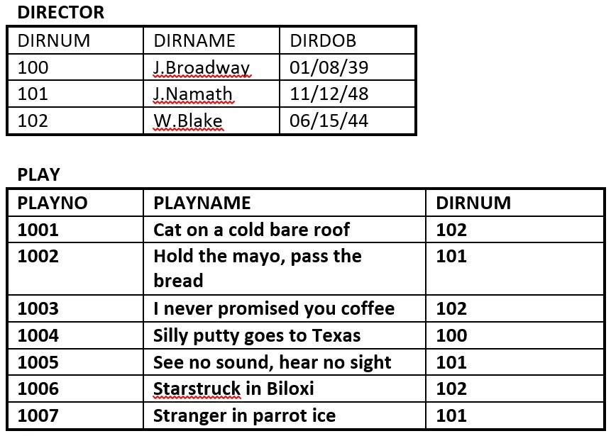
2. The database in Figure 8.11 is composed of two tables. Use this figure to answer questions 2.1 to
2.5.
Figure 8.11. Director and Play tables for question 2, by A. Watt.
2.1 Identify the primary key for each table.
2.2 Identify the foreign key in the PLAY table.
2.3 Identify the candidate keys in both tables.
2.4 Draw the ER model.
2.5 Does the PLAY table exhibit referential integrity? Why or why not?
3. Define the following terms (you may need to use the Internet for some of these):
schema
host language
data sublanguage
data definition language
unary relation
foreign key
virtual relation
connectivity
composite key
linking table
4. The RRE Trucking Company database includes the three tables in Figure 8.12. Use Figure 8.12 to
answer questions 4.1 to 4.5.
40 •
THIS TEXTBOOK IS AVAILABLE FOR FREE AT OPEN.BCCAMPUS.CA
Figure 8.12. Truck, Base and Type tables for question 4, by A. Watt.
4.1 Identify the primary and foreign key(s) for each table.
4.2 Does the TRUCK table exhibit entity and referential integrity? Why or why not? Explain
your answer.
4.3 What kind of relationship exists between the TRUCK and BASE tables?
4.4 How many entities does the TRUCK table contain ?
4.5 Identify the TRUCK table candidate key(s).
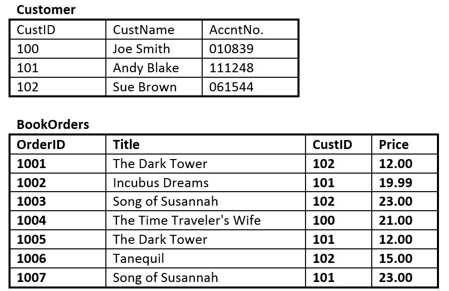
Figure 8.13. Customer and BookOrders tables for question 5, by A. Watt.
5. Suppose you are using the database in Figure 8.13, composed of the two tables. Use Figure 8.13 to
answer questions 5.1 to 5.6.
5.1 Identify the primary key in each table.
5.2 Identify the foreign key in the BookOrders table.
5.3 Are there any candidate keys in either table?
CHAPTER 8 THE ENTITY RELATIONSHIP DATA MODEL • 41
THIS TEXTBOOK IS AVAILABLE FOR FREE AT OPEN.BCCAMPUS.CA
5.4 Draw the ER model.
5.5 Does the BookOrders table exhibit referential integrity? Why or why not?
5.6 Do the tables contain redundant data? If so which table(s) and what is the redundant
data?
6. Looking at the student table in Figure 8.14, list all the possible candidate keys. Why did you select
these?
Figure 8.14. Student table for ques-
tion 6, by A. Watt.
Figure 8.15. ERD of school database for questions 7-10, by A. Watt.
Use the ERD of a school database in Figure 8.15 to answer questions 7 to 10.
7. Identity all the kernels and dependent and characteristic entities in the ERD.
8. Which of the tables contribute to weak relationships? Strong relationships?
42 •
THIS TEXTBOOK IS AVAILABLE FOR FREE AT OPEN.BCCAMPUS.CA
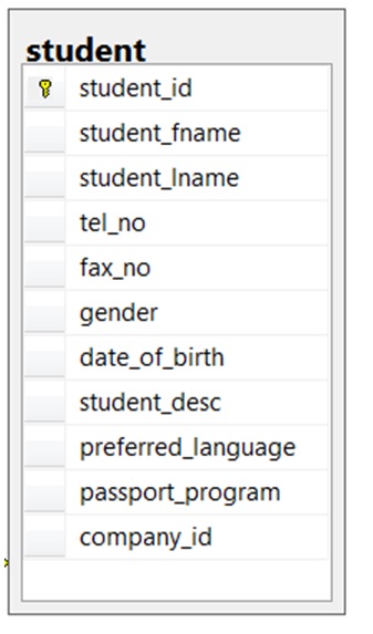
9. Looking at each of the tables in the school database in Figure 8.15, which attribute could have a
NULL value? Why?
10. Which of the tables were created as a result of many to many relationships?
Also see Appendix B: Sample ERD Exercises
Attribution
This chapter of Database Design (including images, except as otherwisse noted) is a derivative copy of Data Modeling
Using Entity-Relationship Model by Nguyen Kim Anh licensed under Creative Commons Attribution License 3.0
license
The following material was written by Adrienne Watt:
1. Nulls section and example
2. Key Terms
3. Exercises
CHAPTER 8 THE ENTITY RELATIONSHIP DATA MODEL • 43
THIS TEXTBOOK IS AVAILABLE FOR FREE AT OPEN.BCCAMPUS.CA
Chapter 9 Integrity Rules and Constraints Adrienne Watt & Nelson Eng
Constraints are a very important feature in a relational model. In fact, the relational model supports the well-defined
theory of constraints on attributes or tables. Constraints are useful because they allow a designer to specify the seman-
tics of data in the database. Constraints are the rules that force DBMSs to check that data satisfies the semantics.
Domain Integrity
Domain restricts the values of attributes in the relation and is a constraint of the relational model. However, there are
real-world semantics for data that cannot be specified if used only with domain constraints. We need more specific ways
to state what data values are or are not allowed and which format is suitable for an attribute. For example, the Employee
ID (EID) must be unique or the employee Birthdate is in the range [ Jan 1, 1950, Jan 1, 2000]. Such information is pro-
vided in logical statements called integrity constraints.
There are several kinds of integrity constraints, described below.
Entity integrity
To ensure entity integrity, it is required that every table have a primary key. Neither the PK nor any part of it can contain
null values. This is because null values for the primary key mean we cannot identify some rows. For example, in the
EMPLOYEE table, Phone cannot be a primary key since some people may not have a telephone.
Referential integrity
Referential integrity requires that a foreign key must have a matching primary key or it must be null. This constraint is
specified between two tables (parent and child); it maintains the correspondence between rows in these tables. It means
the reference from a row in one table to another table must be valid.
Examples of referential integrity constraint in the Customer/Order database of the Company:
• Customer(CustID, CustName)
• Order(OrderID, CustID, OrderDate)
To ensure that there are no orphan records, we need to enforce referential integrity. An orphan record is one whose for-
eign key FK value is not found in the corresponding entity – the entity where the PK is located. Recall that a typical join
is between a PK and FK.
The referential integrity constraint states that the customer ID (CustID) in the Order table must match a valid CustID in
the Customer table. Most relational databases have declarative referential integrity. In other words, when the tables are
created the referential integrity constraints are set up.
Here is another example from a Course/Class database:
• Course(CrsCode, DeptCode, Description)
44
• Class(CrsCode, Section, ClassTime)
The referential integrity constraint states that CrsCode in the Class table must match a valid CrsCode in the Course
table. In this situation, it’s not enough that the CrsCode and Section in the Class table make up the PK, we must also
enforce referential integrity.
When setting up referential integrity it is important that the PK and FK have the same data types and come from the
same domain, otherwise the relational database management system (RDBMS) will not allow the join. RDBMS is a pop-
ular database system that is based on the relational model introduced by E. F. Codd of IBM’s San Jose Research Labora-
tory. Relational database systems are easier to use and understand than other database systems.
Referential integrity in Microsoft Access
In Microsoft (MS) Access, referential integrity is set up by joining the PK in the Customer table to the CustID in the
Order table. See Figure 9.1 for a view of how this is done on the Edit Relationships screen in MS Access.
Figure 9.1. Referential access in MS Access, by A. Watt.
Referential integrity using Transact-SQL (MS SQL Server)
When using Transact-SQL, the referential integrity is set when creating the Order table with the FK. Listed below are
the statements showing the FK in the Order table referencing the PK in the Customer table.
CREATE TABLE Customer
( CustID INTEGER PRIMARY KEY,
CustName CHAR(35) )
CREATE TABLE Orders
( OrderID INTEGER PRIMARY KEY,
CustID INTEGER REFERENCES Customer(CustID),
OrderDate DATETIME )
CHAPTER 9 INTEGRITY RULES AND CONSTRAINTS • 45
THIS TEXTBOOK IS AVAILABLE FOR FREE AT OPEN.BCCAMPUS.CA
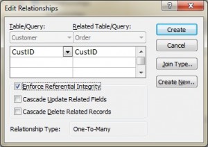
Foreign key rules
Additional foreign key rules may be added when setting referential integrity, such as what to do with the child rows (in
the Orders table) when the record with the PK, part of the parent (Customer), is deleted or changed (updated). For exam-
ple, the Edit Relationships window in MS Access (see Figure 9.1) shows two additional options for FK rules: Cascade
Update and Cascade Delete. If these are not selected, the system will prevent the deletion or update of PK values in the
parent table (Customer table) if a child record exists. The child record is any record with a matching PK.
In some databases, an additional option exists when selecting the Delete option called Set to Null. In this is chosen, the
PK row is deleted, but the FK in the child table is set to NULL. Though this creates an orphan row, it is acceptable.
Enterprise Constraints
Enterprise constraints – sometimes referred to as semantic constraints – are additional rules specified by users or data-
base administrators and can be based on multiple tables.
Here are some examples.
• A class can have a maximum of 30 students.
• A teacher can teach a maximum of four classes per semester.
• An employee cannot take part in more than five projects.
• The salary of an employee cannot exceed the salary of the employee’s manager.
Business Rules
Business rules are obtained from users when gathering requirements. The requirements-gathering process is very impor-
tant, and its results should be verified by the user before the database design is built. If the business rules are incorrect,
the design will be incorrect, and ultimately the application built will not function as expected by the users.
Some examples of business rules are:
• A teacher can teach many students.
• A class can have a maximum of 35 students.
• A course can be taught many times, but by only one instructor.
• Not all teachers teach classes.
Cardinality and connectivity
Business rules are used to determine cardinality and connectivity. Cardinality describes the relationship between two
data tables by expressing the minimum and maximum number of entity occurrences associated with one occurrence of
a related entity. In Figure 9.2, you can see that cardinality is represented by the innermost markings on the relationship
symbol. In this figure, the cardinality is 0 (zero) on the right and 1 (one) on the left.
The outermost symbol of the relationship symbol, on the other hand, represents the connectivity between the two
tables. Connectivity is the relationship between two tables, e.g., one to one or one to many. The only time it is zero is
when the FK can be null. When it comes to participation, there are three options to the relationship between these enti-
ties: either 0 (zero), 1 (one) or many. In Figure 9.2, for example, the connectivity is 1 (one) on the outer, left-hand side of
this line and many on the outer, right-hand side.
46 •
THIS TEXTBOOK IS AVAILABLE FOR FREE AT OPEN.BCCAMPUS.CA
Figure 9.2. Position of connectivity and cardinality on a relationship
symbol, by A. Watt.
Figure 9.3. shows the symbol that represents a one to many relationship.
Figure 9.3.
In Figure 9.4, both inner (representing cardinality) and outer (representing connectivity) markers are shown. The left
side of this symbol is read as minimum 1 and maximum 1. On the right side, it is read as: minimum 1 and maximum
many.
Figure 9.4.
Relationship Types
The line that connects two tables, in an ERD, indicates the relationship type between the tables: either identifying or non-
identifying. An identifying relationship will have a solid line (where the PK contains the FK). A non-identifying relationship
is indicated by a broken line and does not contain the FK in the PK. See the section in Chapter 8 that discusses weak and
strong relationships for more explanation.
Optional relationships
In an optional relationship, the FK can be null or the parent table does not need to have a corresponding child table occur-
rence. The symbol, shown in Figure 9.6, illustrates one type with a zero and three prongs (indicating many) which is
interpreted as zero OR many.
Figure 9.6.
CHAPTER 9 INTEGRITY RULES AND CONSTRAINTS • 47
THIS TEXTBOOK IS AVAILABLE FOR FREE AT OPEN.BCCAMPUS.CA
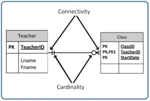
Figure 9.5. Identifying and non-identifying relationship, by A. Watt.
For example, if you look at the Order table on the right-hand side of Figure 9.7, you’ll notice that a customer doesn’t
need to place an order to be a customer. In other words, the many side is optional.
Figure 9.7. Example usage of a zero to many optional relationship sym-
bol, by A. Watt.
The relationship symbol in Figure 9.7 can also be read as follows:
• Left side: The order entity must contain a minimum of one related entity in the Customer table and a
maximum of one related entity.
• Right side: A customer can place a minimum of zero orders or a maximum of many orders.
Figure 9.8 shows another type of optional relationship symbol with a zero and one, meaning zero OR one. The
one side is optional.
Figure 9.9 gives an example of how a zero to one symbol might be used.
48 •
THIS TEXTBOOK IS AVAILABLE FOR FREE AT OPEN.BCCAMPUS.CA
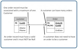
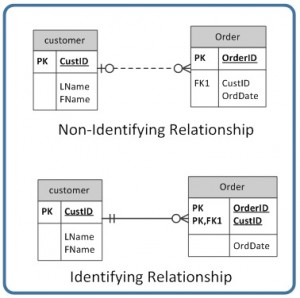
Figure 9.8.
Figure 9.9. Example usage of a zero to one optional relationship symbol,
by A. Watt.
Mandatory relationships
In a mandatory relationship, one entity occurrence requires a corresponding entity occurrence. The symbol for this rela-
tionship shows one and only one as shown in Figure 9.10. The one side is mandatory.
Figure 9.10
See Figure 9.11 for an example of how the one and only one mandatory symbol is used.
Figure 9.11. Example of a one and only one mandatory relationship
symbol, by A. Watt.
CHAPTER 9 INTEGRITY RULES AND CONSTRAINTS • 49
THIS TEXTBOOK IS AVAILABLE FOR FREE AT OPEN.BCCAMPUS.CA
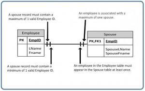
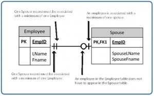
Figure 9.12 illustrates what a one to many relationship symbol looks like where the many side is mandatory.
Figure
9.12.
Refer to Figure 9.13 for an example of how the one to many symbol may be used.
Figure 9.13. Example of a one to many mandatory relationship symbol,
by A. Watt.
So far we have seen that the innermost side of a relationship symbol (on the left-side of the symbol in Figure 9.14) can
have a 0 (zero) cardinality and a connectivity of many (shown on the right-side of the symbol in Figure 9.14), or one (not
shown).
Figure 9.14
However, it cannot have a connectivity of 0 (zero), as displayed in Figure 9.15. The connectivity can only be 1.
Figure 9.15.
The connectivity symbols show maximums. So if you think about it logically, if the connectivity symbol on the left side
shows 0 (zero), then there would be no connection between the tables.
The way to read a relationship symbol, such as the one in Figure 9.16, is as follows.
• The CustID in the Order table must also be found in the Customer table a minimum of 0 and a maximum of
1 times.
• The 0 means that the CustID in the Order table may be null.
50 •
THIS TEXTBOOK IS AVAILABLE FOR FREE AT OPEN.BCCAMPUS.CA
• The left-most 1 (right before the 0 representing connectivity) says that if there is a CustID in the Order table,
it can only be in the Customer table once.
• When you see the 0 symbol for cardinality, you can assume two things: T
1. the FK in the Order table allows nulls, and
2. the FK is not part of the PK since PKs must not contain null values.
Figure 9.16. The relationship between a Customer table and an Order
table, by A. Watt.
Key Terms
business rules: obtained from users when gathering requirements and are used to determine cardinality
cardinality: expresses the minimum and maximum number of entity occurrences associated with one occur-
rence of a related entity
connectivity: the relationship between two tables, e.g., one to one or one to many
constraints: the rules that force DBMSs to check that data satisfies the semantics
entity integrity: requires that every table have a primary key; neither the primary key, nor any part of it, can
contain null values
identifying relationship: where the primary key contains the foreign key; indicated in an ERD by a solid line
integrity constraints: logical statements that state what data values are or are not allowed and which format is
suitable for an attribute
mandatory relationship: one entity occurrence requires a corresponding entity occurrence.
non-identifying relationship: does not contain the foreign key in the primary key; indicated in an ERD by a
dotted line
CHAPTER 9 INTEGRITY RULES AND CONSTRAINTS • 51
THIS TEXTBOOK IS AVAILABLE FOR FREE AT OPEN.BCCAMPUS.CA
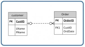
optional relationship: the FK can be null or the parent table does not need to have a corresponding child
table occurrence
orphan record: a record whose foreign key value is not found in the corresponding entity – the entity where
the primary key is located
referential integrity: requires that a foreign key must have a matching primary key or it must be null
relational database management system (RDBMS): a popular database system based on the relational model
introduced by E. F. Codd of IBM’s San Jose Research Laboratory
relationship type: the type of relationship between two tables in an ERD (either identifying or non-identifying);
this relationship is indicated by a line drawn between the two tables.
Exercises
Read the following description and then answer questions 1-5 at the end.
The swim club database in Figure 9.17 has been designed to hold information about students who are enrolled
in swim classes. The following information is stored: students, enrollment, swim classes, pools where classes are
held, instructors for the classes, and various levels of swim classes. Use Figure 9.17 to answer questions 1 to 5.
Figure 9.17. ERD for questions 1-5. (Diagram by A. Watt.)
The primary keys are identified below. The following data types are defined in the SQL Server.
52 •
THIS TEXTBOOK IS AVAILABLE FOR FREE AT OPEN.BCCAMPUS.CA
tblLevels
Level – Identity PK
ClassName – text 20 – nulls are not allowed
tblPool
Pool – Identity PK
PoolName – text 20 – nulls are not allowed
Location – text 30
tblStaff
StaffID – Identity PK
FirstName – text 20
MiddleInitial – text 3
LastName – text 30
Suffix – text 3
Salaried – Bit
PayAmount – money
tblClasses
LessonIndex – Identity PK
Level – Integer FK
SectionID – Integer
Semester – TinyInt
Days – text 20
Time – datetime (formatted for time)
Pool – Integer FK
Instructor – Integer FK
Limit – TinyInt
Enrolled – TinyInt
Price – money
tblEnrollment
LessonIndex – Integer FK
SID – Integer FK (LessonIndex and SID) Primary Key
Status – text 30
Charged – bit
AmountPaid – money
DateEnrolled – datetime
tblStudents
SID – Identity PK
FirstName – text 20
MiddleInitial – text 3
LastName – text 30
Suffix – text 3
Birthday – datetime
LocalStreet – text 30
LocalCity – text 20
CHAPTER 9 INTEGRITY RULES AND CONSTRAINTS • 53
THIS TEXTBOOK IS AVAILABLE FOR FREE AT OPEN.BCCAMPUS.CA
LocalPostalCode – text 6
LocalPhone – text 10
Implement this schema in SQL Server or access (you will need to pick comparable data types). Submit a screen-
shot of your ERD in the database.
1. Explain the relationship rules for each relationship (e.g., tblEnrollment and tblStudents: A student
can enroll in many classes).
2. Identify cardinality for each relationship, assuming the following rules:
◦ 2.1 A pool may or may not ever have a class. ◦ 2.1 The levels table must always be associated with at least one class. ◦ 2.1 The staff table may not have ever taught a class. ◦ 2.1 All students must be enrolled in at least one class. ◦ 2.1 The class must have students enrolled in it. ◦ 2.1 The class must have a valid pool. ◦ 2.1 The class may not have an instructor assigned. ◦ 2.1 The class must always be associated with an existing level.
3. Which tables are weak and which tables are strong (covered in an earlier chapter)?
4. Which of the tables are non-identifying and which are identifying?
Image Attributions
Figures 9.3, 9.4, 9.6, 9.8, 9.10, 9.12, 9.14 and 9.15 by A. Watt.
54 •
THIS TEXTBOOK IS AVAILABLE FOR FREE AT OPEN.BCCAMPUS.CA
Chapter 10 ER Modelling Adrienne Watt
One important theory developed for the entity relational (ER) model involves the notion of functional dependency (FD).
The aim of studying this is to improve your understanding of relationships among data and to gain enough formalism
to assist with practical database design.
Like constraints, FDs are drawn from the semantics of the application domain. Essentially, functional dependencies
describe how individual attributes are related. FDs are a kind of constraint among attributes within a relation and con-
tribute to a good relational schema design. In this chapter, we will look at:
• The basic theory and definition of functional dependency
• The methodology for improving schema designs, also called normalization
Relational Design and Redundancy
Generally, a good relational database design must capture all of the necessary attributes and associations. The design
should do this with a minimal amount of stored information and no redundant data.
In database design, redundancy is generally undesirable because it causes problems maintaining consistency after
updates. However, redundancy can sometimes lead to performance improvements; for example, when redundancy can
be used in place of a join to connect data. A join is used when you need to obtain information based on two related tables.
Consider Figure 10.1: customer 1313131 is displayed twice, once for account no. A-101 and again for account A-102.
In this case, the customer number is not redundant, although there are deletion anomalies with the table. Having a sepa-
rate customer table would solve this problem. However, if a branch address were to change, it would have to be updated
in multiple places. If the customer number was left in the table as is, then you wouldn’t need a branch table and no join
would be required, and performance is improved .
Figure 10.1. An example of redundancy used with bank accounts and
branches.
55
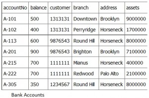
Insertion Anomaly
An insertion anomaly occurs when you are inserting inconsistent information into a table. When we insert a new record,
such as account no. A-306 in Figure 10.2, we need to check that the branch data is consistent with existing rows.
Figure 10.2. Example of an insertion anomaly.
Update Anomaly
If a branch changes address, such as the Round Hill branch in Figure 10.3, we need to update all rows referring to that
branch. Changing existing information incorrectly is called an update anomaly.
Figure 10.3. Example of an update anomaly.
Deletion Anomaly
A deletion anomaly occurs when you delete a record that may contain attributes that shouldn’t be deleted. For instance,
if we remove information about the last account at a branch, such as account A-101 at the Downtown branch in Figure
10.4, all of the branch information disappears.
56 •
THIS TEXTBOOK IS AVAILABLE FOR FREE AT OPEN.BCCAMPUS.CA
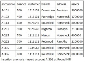
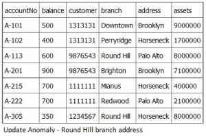
Figure 10.4. Example of a deletion anomaly.
The problem with deleting the A-101 row is we don’t know where the Downtown branch is located and we lose all
information regarding customer 1313131. To avoid these kinds of update or deletion problems, we need to decompose
the original table into several smaller tables where each table has minimal overlap with other tables.
Each bank account table must contain information about one entity only, such as the Branch or Customer, as displayed
in Figure 10.5.
Figure 10.5. Examples of bank account tables that contain one entity
each, by A. Watt.
Following this practice will ensure that when branch information is added or updated it will only affect one record. So,
when customer information is added or deleted, the branch information will not be accidentally modified or incorrectly
recorded.
Example: employee project table and anomalies
Figure 10.6 shows an example of an employee project table. From this table, we can assume that:
1. EmpID and ProjectID are a composite PK.
2. Project ID determines Budget (i.e., Project P1 has a budget of 32 hours).
Next, let’s look at some possible anomalies that might occur with this table during the following steps.
1. Action: Add row {S85,35,P1,9}
2. Problem: There are two tuples with conflicting budgets
3. Action: Delete tuple {S79, 27, P3, 1}
4. Problem: Step #3 deletes the budget for project P3
5. Action: Update tuple {S75, 32, P1, 7} to {S75, 35, P1, 7}
CHAPTER 10 ER MODELLING • 57
THIS TEXTBOOK IS AVAILABLE FOR FREE AT OPEN.BCCAMPUS.CA
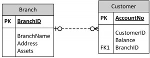
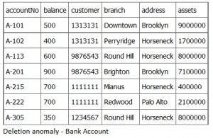
Figure 10.6. Example of an employee project table, by A. Watt.
6. Problem: Step #5 creates two tuples with different values for project P1’s budget
7. Solution: Create a separate table, each, for Projects and Employees, as shown in Figure 10.7.
Figure 10.7. Solution: separate tables for Project and Employee, by A.
Watt.
How to Avoid Anomalies
The best approach to creating tables without anomalies is to ensure that the tables are normalized, and that’s accom-
plished by understanding functional dependencies. FD ensures that all attributes in a table belong to that table. In other
words, it will eliminate redundancies and anomalies.
Example: separate Project and Employee tables
Figure 10.8. Separate Project and Employee tables with data, by A. Watt.
By keeping data separate using individual Project and Employee tables:
1. No anomalies will be created if a budget is changed.
2. No dummy values are needed for projects that have no employees assigned.
3. If an employee’s contribution is deleted, no important data is lost.
4. No anomalies are created if an employee’s contribution is added.
58 •
THIS TEXTBOOK IS AVAILABLE FOR FREE AT OPEN.BCCAMPUS.CA
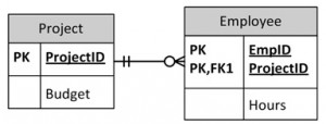
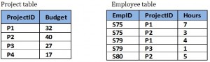
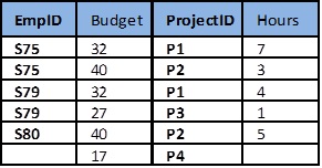
Key Terms
deletion anomaly: occurs when you delete a record that may contain attributes that shouldn’t be deleted
functional dependency (FD): describes how individual attributes are related
insertion anomaly: occurs when you are inserting inconsistent information into a table
join: used when you need to obtain information based on two related tables
update anomaly: changing existing information incorrectly
Exercises
1. Normalize Figure 10.9.
Figure 10.9. Table for question 1, by A. Watt.
2. Create a logical ERD for an online movie rental service (no many to many relationships). Use the
following description of operations on which your business rules must be based:The online movie
rental service classifies movie titles according to their type: comedy, western, classical, science fiction,
cartoon, action, musical, and new release. Each type contains many possible titles, and most titles
within a type are available in multiple copies. For example, note the following summary:TYPE TITLE
Musical My Fair Lady (Copy 1)
My Fair Lady (Copy 2)
Oklahoma (Copy 1)
Oklahoma (Copy 2)
Oklahoma (Copy 3)
etc.
3. What three data anomalies are likely to be the result of data redundancy? How can such anomalies
be eliminated?
Also see Appendix B: Sample ERD Exercises
CHAPTER 10 ER MODELLING • 59
THIS TEXTBOOK IS AVAILABLE FOR FREE AT OPEN.BCCAMPUS.CA
Attribution
This chapter of Database Design (including images, except as otherwise noted) is a derivative copy of Relational Design
Theory by Nguyen Kim Anh licensed under Creative Commons Attribution License 3.0 license
The following material was written by Adrienne Watt:
1. Example: employee project table and anomalies
2. How to Avoid Anomalies
3. Key Terms
4. Exercises
60 •
THIS TEXTBOOK IS AVAILABLE FOR FREE AT OPEN.BCCAMPUS.CA
Chapter 11 Functional Dependencies Adrienne Watt
A functional dependency (FD) is a relationship between two attributes, typically between the PK and other non-key attrib-
utes within a table. For any relation R, attribute Y is functionally dependent on attribute X (usually the PK), if for every
valid instance of X, that value of X uniquely determines the value of Y. This relationship is indicated by the representa-
tion below :
X ———–> Y
The left side of the above FD diagram is called the determinant, and the right side is the dependent. Here are a few exam-
ples.
In the first example, below, SIN determines Name, Address and Birthdate. Given SIN, we can determine any of the other
attributes within the table.
SIN ———-> Name, Address, Birthdate
For the second example, SIN and Course determine the date completed (DateCompleted). This must also work for a
composite PK.
SIN, Course ———> DateCompleted
The third example indicates that ISBN determines Title.
ISBN ———–> Title
Rules of Functional Dependencies
Consider the following table of data r(R) of the relation schema R(ABCDE) shown in Table 11.1.
As you look at this table, ask yourself: What kind of dependencies can we observe among the attributes in Table R? Since the
values of A are unique (a1, a2, a3, etc.), it follows from the FD definition that:
A → B, A → C, A → D, A → E
• It also follows that A →BC (or any other subset of ABCDE).
• This can be summarized as A →BCDE.
• From our understanding of primary keys, A is a primary key.
Since the values of E are always the same (all e1), it follows that:
61
Table 11.1. Functional dependency
example, by A. Watt.
A → E, B → E, C → E, D → E
However, we cannot generally summarize the above with ABCD → E because, in general, A → E, B → E, AB → E.
Other observations:
1. Combinations of BC are unique, therefore BC → ADE.
2. Combinations of BD are unique, therefore BD → ACE.
3. If C values match, so do D values.
3.1 Therefore, C → D
3.2 However, D values don’t determine C values
3.3 So C does not determine D, and D does not determine C.
Looking at actual data can help clarify which attributes are dependent and which are determinants.
Inference Rules
Armstrong’s axioms are a set of inference rules used to infer all the functional dependencies on a relational database. They
were developed by William W. Armstrong. The following describes what will be used, in terms of notation, to explain
these axioms.
Let R(U) be a relation scheme over the set of attributes U. We will use the letters X, Y, Z to represent any subset of and,
for short, the union of two sets of attributes, instead of the usual X U Y.
Axiom of reflexivity
This axiom says, if Y is a subset of X, then X determines Y (see Figure 11.1).
For example, PartNo —> NT123 where X (PartNo) is composed of more than one piece of information; i.e., Y (NT) and
partID (123).
62 •
THIS TEXTBOOK IS AVAILABLE FOR FREE AT OPEN.BCCAMPUS.CA
Figure 11.1. Equation for axiom of reflexivity.
Axiom of augmentation
The axiom of augmentation, also known as a partial dependency, says if X determines Y, then XZ determines YZ for any
Z (see Figure 11.2 ).
Figure 11.2. Equation for axiom of augmentation.
The axiom of augmentation says that every non-key attribute must be fully dependent on the PK. In the example shown
below, StudentName, Address, City, Prov, and PC (postal code) are only dependent on the StudentNo, not on the Stu-
dentNo and Grade.
StudentNo, Course —> StudentName, Address, City, Prov, PC, Grade, DateCompleted
This situation is not desirable because every non-key attribute has to be fully dependent on the PK. In this situation, stu-
dent information is only partially dependent on the PK (StudentNo).
To fix this problem, we need to break the original table down into two as follows:
• Table 1: StudentNo, Course, Grade, DateCompleted
• Table 2: StudentNo, StudentName, Address, City, Prov, PC
Axiom of transitivity
The axiom of transitivity says if X determines Y, and Y determines Z, then X must also determine Z (see Figure 11.3).
Figure 11.3. Equation for axiom of transitivity.
The table below has information not directly related to the student; for instance, ProgramID and ProgramName should
have a table of its own. ProgramName is not dependent on StudentNo; it’s dependent on ProgramID.
StudentNo —> StudentName, Address, City, Prov, PC, ProgramID, ProgramName
This situation is not desirable because a non-key attribute (ProgramName) depends on another non-key attribute (Pro-
gramID).
To fix this problem, we need to break this table into two: one to hold information about the student and the other to
hold information about the program.
• Table 1: StudentNo —> StudentName, Address, City, Prov, PC, ProgramID
CHAPTER 11 FUNCTIONAL DEPENDENCIES • 63
THIS TEXTBOOK IS AVAILABLE FOR FREE AT OPEN.BCCAMPUS.CA
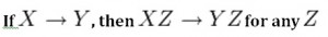
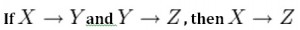
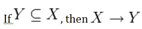
• Table 2: ProgramID —> ProgramName
However we still need to leave an FK in the student table so that we can identify which program the student is enrolled
in.
Union
This rule suggests that if two tables are separate, and the PK is the same, you may want to consider putting them togeth-
er. It states that if X determines Y and X determines Z then X must also determine Y and Z (see Figure 11.4).
Figure 11.4. Equation for the Union rule.
For example, if:
• SIN —> EmpName
• SIN —> SpouseName
You may want to join these two tables into one as follows:
SIN –> EmpName, SpouseName
Some database administrators (DBA) might choose to keep these tables separated for a couple of reasons. One, each table
describes a different entity so the entities should be kept apart. Two, if SpouseName is to be left NULL most of the time,
there is no need to include it in the same table as EmpName.
Decomposition
Decomposition is the reverse of the Union rule. If you have a table that appears to contain two entities that are deter-
mined by the same PK, consider breaking them up into two tables. This rule states that if X determines Y and Z, then X
determines Y and X determines Z separately (see Figure 11.5).
Figure 11.5. Equation for decompensation rule.
Dependency Diagram
A dependency diagram, shown in Figure 11.6, illustrates the various dependencies that might exist in a non-normalized
table. A non-normalized table is one that has data redundancy in it.
Figure 11.6. Dependency diagram.
The following dependencies are identified in this table:
64 •
THIS TEXTBOOK IS AVAILABLE FOR FREE AT OPEN.BCCAMPUS.CA
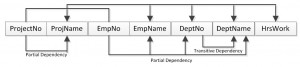
• ProjectNo and EmpNo, combined, are the PK.
• Partial Dependencies:
ProjectNo —> ProjName
EmpNo —> EmpName, DeptNo,
ProjectNo, EmpNo —> HrsWork
• Transitive Dependency:
DeptNo —> DeptName
Key Terms
Armstrong’s axioms: a set of inference rules used to infer all the functional dependencies on a relational data-
base
DBA: database administrator
decomposition: a rule that suggests if you have a table that appears to contain two entities that are determined
by the same PK, consider breaking them up into two tables
dependent: the right side of the functional dependency diagram
determinant: the left side of the functional dependency diagram
functional dependency (FD): a relationship between two attributes, typically between the PK and other non-
key attributes within a table
non-normalized table: a table that has data redundancy in it
Union: a rule that suggests that if two tables are separate, and the PK is the same, consider putting them together
Exercises
See Chapter 12.
Attributions
This chapter of Database Design (including images, except as otherwise noted) is a derivative copy of Armstrong’s
axioms by Wikipedia the Free Encyclopedia licensed under Creative Commons Attribution-ShareAlike 3.0 Unported
The following material was written by Adrienne Watt:
1. some of Rules of Functional Dependencies
2. Key Terms
CHAPTER 11 FUNCTIONAL DEPENDENCIES • 65
THIS TEXTBOOK IS AVAILABLE FOR FREE AT OPEN.BCCAMPUS.CA
Chapter 12 Normalization Adrienne Watt
Normalization should be part of the database design process. However, it is difficult to separate the normalization
process from the ER modelling process so the two techniques should be used concurrently.
Use an entity relation diagram (ERD) to provide the big picture, or macro view, of an organization’s data requirements
and operations. This is created through an iterative process that involves identifying relevant entities, their attributes
and their relationships.
Normalization procedure focuses on characteristics of specific entities and represents the micro view of entities within
the ERD.
What Is Normalization?
Normalization is the branch of relational theory that provides design insights. It is the process of determining how much
redundancy exists in a table. The goals of normalization are to:
• Be able to characterize the level of redundancy in a relational schema
• Provide mechanisms for transforming schemas in order to remove redundancy
Normalization theory draws heavily on the theory of functional dependencies. Normalization theory defines six normal
forms (NF). Each normal form involves a set of dependency properties that a schema must satisfy and each normal
form gives guarantees about the presence and/or absence of update anomalies. This means that higher normal forms
have less redundancy, and as a result, fewer update problems.
Normal Forms
All the tables in any database can be in one of the normal forms we will discuss next. Ideally we only want minimal
redundancy for PK to FK. Everything else should be derived from other tables. There are six normal forms, but we will
only look at the first four, which are:
• First normal form (1NF)
• Second normal form (2NF)
• Third normal form (3NF)
• Boyce-Codd normal form (BCNF)
BCNF is rarely used.
First Normal Form (1NF)
In the first normal form, only single values are permitted at the intersection of each row and column; hence, there are no
repeating groups.
To normalize a relation that contains a repeating group, remove the repeating group and form two new relations.
66
The PK of the new relation is a combination of the PK of the original relation plus an attribute from the newly created
relation for unique identification.
Process for 1NF
We will use the Student_Grade_Report table below, from a School database, as our example to explain the process for
1NF.
Student_Grade_Report (StudentNo, StudentName, Major, CourseNo, CourseName, InstructorNo,
InstructorName, InstructorLocation, Grade)
• In the Student Grade Report table, the repeating group is the course information. A student can take many
courses.
• Remove the repeating group. In this case, it’s the course information for each student.
• Identify the PK for your new table.
• The PK must uniquely identify the attribute value (StudentNo and CourseNo).
• After removing all the attributes related to the course and student, you are left with the student course table
(StudentCourse).
• The Student table (Student) is now in first normal form with the repeating group removed.
• The two new tables are shown below.
Student (StudentNo, StudentName, Major)
StudentCourse (StudentNo, CourseNo, CourseName, InstructorNo, InstructorName, InstructorLocation, Grade)
How to update 1NF anomalies
StudentCourse (StudentNo, CourseNo, CourseName, InstructorNo, InstructorName, InstructorLocation, Grade)
• To add a new course, we need a student.
• When course information needs to be updated, we may have inconsistencies.
• To delete a student, we might also delete critical information about a course.
Second Normal Form (2NF)
For the second normal form, the relation must first be in 1NF. The relation is automatically in 2NF if, and only if, the PK
comprises a single attribute.
If the relation has a composite PK, then each non-key attribute must be fully dependent on the entire PK and not on a
subset of the PK (i.e., there must be no partial dependency or augmentation).
CHAPTER 12 NORMALIZATION • 67
THIS TEXTBOOK IS AVAILABLE FOR FREE AT OPEN.BCCAMPUS.CA
Process for 2NF
To move to 2NF, a table must first be in 1NF.
• The Student table is already in 2NF because it has a single-column PK.
• When examining the Student Course table, we see that not all the attributes are fully dependent on the PK;
specifically, all course information. The only attribute that is fully dependent is grade.
• Identify the new table that contains the course information.
• Identify the PK for the new table.
• The three new tables are shown below.
Student (StudentNo, StudentName, Major)
CourseGrade (StudentNo, CourseNo, Grade)
CourseInstructor (CourseNo, CourseName, InstructorNo, InstructorName, InstructorLocation)
How to update 2NF anomalies
• When adding a new instructor, we need a course.
• Updating course information could lead to inconsistencies for instructor information.
• Deleting a course may also delete instructor information.
Third Normal Form (3NF)
To be in third normal form, the relation must be in second normal form. Also all transitive dependencies must be
removed; a non-key attribute may not be functionally dependent on another non-key attribute.
Process for 3NF
• Eliminate all dependent attributes in transitive relationship(s) from each of the tables that have a transitive
relationship.
• Create new table(s) with removed dependency.
• Check new table(s) as well as table(s) modified to make sure that each table has a determinant and that no
table contains inappropriate dependencies.
• See the four new tables below.
Student (StudentNo, StudentName, Major)
CourseGrade (StudentNo, CourseNo, Grade)
68 •
THIS TEXTBOOK IS AVAILABLE FOR FREE AT OPEN.BCCAMPUS.CA
Course (CourseNo, CourseName, InstructorNo)
Instructor (InstructorNo, InstructorName, InstructorLocation)
At this stage, there should be no anomalies in third normal form. Let’s look at the dependency diagram (Figure 12.1) for
this example. The first step is to remove repeating groups, as discussed above.
Student (StudentNo, StudentName, Major)
StudentCourse (StudentNo, CourseNo, CourseName, InstructorNo, InstructorName, InstructorLocation, Grade)
To recap the normalization process for the School database, review the dependencies shown in Figure 12.1.
Figure 12.1 Dependency diagram, by A. Watt.
The abbreviations used in Figure 12.1 are as follows:
• PD: partial dependency
• TD: transitive dependency
• FD: full dependency (Note: FD typically stands for functional dependency. Using FD as an abbreviation for
full dependency is only used in Figure 12.1.)
Boyce-Codd Normal Form (BCNF)
When a table has more than one candidate key, anomalies may result even though the relation is in 3NF. Boyce-Codd
normal form is a special case of 3NF. A relation is in BCNF if, and only if, every determinant is a candidate key.
BCNF Example 1
Consider the following table (St_Maj_Adv).
Student_id Major Advisor
111 Physics Smith
111 Music Chan
320 Math Dobbs
671 Physics White
803 Physics Smith
CHAPTER 12 NORMALIZATION • 69
THIS TEXTBOOK IS AVAILABLE FOR FREE AT OPEN.BCCAMPUS.CA
The semantic rules (business rules applied to the database) for this table are:
1. Each Student may major in several subjects.
2. For each Major, a given Student has only one Advisor.
3. Each Major has several Advisors.
4. Each Advisor advises only one Major.
5. Each Advisor advises several Students in one Major.
The functional dependencies for this table are listed below. The first one is a candidate key; the second is not.
1. Student_id, Major ——> Advisor
2. Advisor ——> Major
Anomalies for this table include:
1. Delete – student deletes advisor info
2. Insert – a new advisor needs a student
3. Update – inconsistencies
Note: No single attribute is a candidate key.
PK can be Student_id, Major or Student_id, Advisor.
To reduce the St_Maj_Adv relation to BCNF, you create two new tables:
1. St_Adv (Student_id, Advisor)
2. Adv_Maj (Advisor, Major)
St_Adv table
Student_id Advisor
111 Smith
111 Chan
320 Dobbs
671 White
803 Smith
Adv_Maj table
Advisor Major
Smith Physics
Chan Music
Dobbs Math
White Physics
BCNF Example 2
Consider the following table (Client_Interview).
70 •
THIS TEXTBOOK IS AVAILABLE FOR FREE AT OPEN.BCCAMPUS.CA
ClientNo InterviewDate InterviewTime StaffNo RoomNo
CR76 13-May-02 10.30 SG5 G101
CR56 13-May-02 12.00 SG5 G101
CR74 13-May-02 12.00 SG37 G102
CR56 1-July-02 10.30 SG5 G102
FD1 – ClientNo, InterviewDate –> InterviewTime, StaffNo, RoomNo (PK)
FD2 – staffNo, interviewDate, interviewTime –> clientNO (candidate key: CK)
FD3 – roomNo, interviewDate, interviewTime –> staffNo, clientNo (CK)
FD4 – staffNo, interviewDate –> roomNo
A relation is in BCNF if, and only if, every determinant is a candidate key. We need to create a table that incorporates
the first three FDs (Client_Interview2 table) and another table (StaffRoom table) for the fourth FD.
Client_Interview2 table
ClientNo InterviewDate InterViewTime StaffNo
CR76 13-May-02 10.30 SG5
CR56 13-May-02 12.00 SG5
CR74 13-May-02 12.00 SG37
CR56 1-July-02 10.30 SG5
StaffRoom table
StaffNo InterviewDate RoomNo
SG5 13-May-02 G101
SG37 13-May-02 G102
SG5 1-July-02 G102
Normalization and Database Design
During the normalization process of database design, make sure that proposed entities meet required normal form
before table structures are created. Many real-world databases have been improperly designed or burdened with anom-
alies if improperly modified during the course of time. You may be asked to redesign and modify existing databases. This
can be a large undertaking if the tables are not properly normalized.
Key Terms and Abbreviations
Boyce-Codd normal form (BCNF): a special case of 3rd NF
CHAPTER 12 NORMALIZATION • 71
THIS TEXTBOOK IS AVAILABLE FOR FREE AT OPEN.BCCAMPUS.CA
first normal form (1NF): only single values are permitted at the intersection of each row and column so there
are no repeating groups
normalization: the process of determining how much redundancy exists in a table
second normal form (2NF): the relation must be in 1NF and the PK comprises a single attribute
semantic rules: business rules applied to the database
third normal form (3NF): the relation must be in 2NF and all transitive dependencies must be removed; a non-
key attribute may not be functionally dependent on another non-key attribute
Exercises
Complete chapters 11 and 12 before doing these exercises.
1. What is normalization?
2. When is a table in 1NF?
3. When is a table in 2NF?
4. When is a table in 3NF?
5. Identify and discuss each of the indicated dependencies in the dependency diagram shown in
Figure 12.2.
Figure 12.2 For question 5, by A. Watt.
6. To keep track of students and courses, a new college uses the table structure in Figure 12.3.
Draw the dependency diagram for this table.
Figure 12.3 For question 6, by A. Watt.
72 •
THIS TEXTBOOK IS AVAILABLE FOR FREE AT OPEN.BCCAMPUS.CA
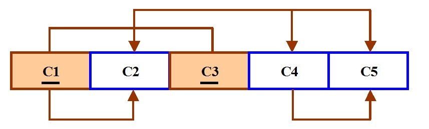
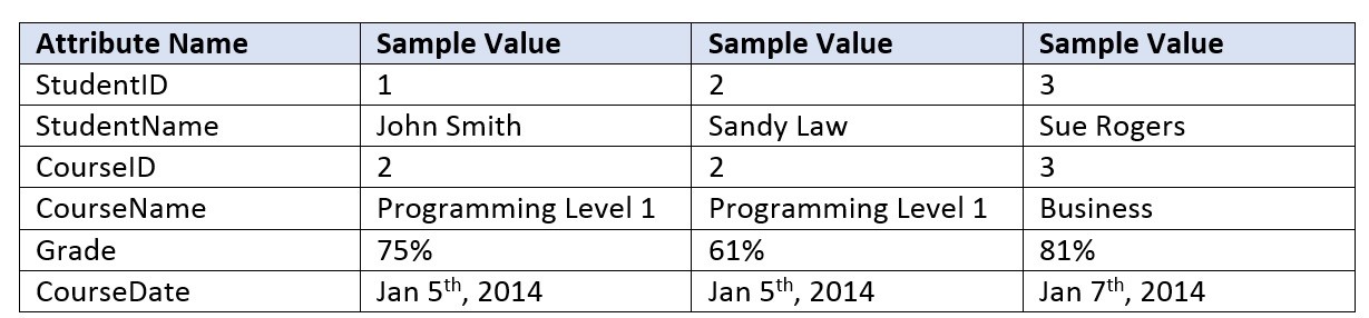
7. Using the dependency diagram you just drew, show the tables (in their third normal form) you
would create to fix the problems you encountered. Draw the dependency diagram for the fixed table.
8. An agency called Instant Cover supplies part-time/temporary staff to hotels in Scotland. Figure
12.4 lists the time spent by agency staff working at various hotels. The national insurance number
(NIN) is unique for every member of staff. Use Figure 12.4 to answer questions (a) and (b).
Figure 12.4 For question 8, by A. Watt.
8.1 This table is susceptible to update anomalies. Provide examples of insertion, deletion
and update anomalies.
8.2 Normalize this table to third normal form. State any assumptions.
9. Fill in the blanks:
9.1 ____________________ produces a lower normal form.
9.2 Any attribute whose value determines other values within a row is called a(n)
____________________.
9.3 An attribute that cannot be further divided is said to display ____________________.
9.4 ____________________ refers to the level of detail represented by the values stored in
a table’s row.
9.5 A relational table must not contain ____________________ groups.
Also see Appendix B: Sample ERD Exercises
Bibliography
Nguyen Kim Anh, Relational Design Theory. OpenStax CNX. 8 Jul 2009 Retrieved July 2014 from http://cnx.org/con-
tents/606cc532-0b1d-419d-a0ec-ac4e2e2d533b@1@1
Russell, Gordon. Chapter 4 – Normalisation. Database eLearning. N.d. Retrived July 2014 from db.grussell.org/ch4.html
CHAPTER 12 NORMALIZATION • 73
THIS TEXTBOOK IS AVAILABLE FOR FREE AT OPEN.BCCAMPUS.CA
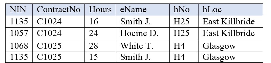
Chapter 13 Database Development Process Adrienne Watt
A core aspect of software engineering is the subdivision of the development process into a series of phases, or steps, each
of which focuses on one aspect of the development. The collection of these steps is sometimes referred to as the software
development life cycle (SDLC). The software product moves through this life cycle (sometimes repeatedly as it is refined or
redeveloped) until it is finally retired from use. Ideally, each phase in the life cycle can be checked for correctness before
moving on to the next phase.
Software Development Life Cycle – Waterfall
Let us start with an overview of the waterfall model such as you will find in most software engineering textbooks. This
waterfall figure, seen in Figure 13.1, illustrates a general waterfall model that could apply to any computer system devel-
opment. It shows the process as a strict sequence of steps where the output of one step is the input to the next and all of
one step has to be completed before moving onto the next.
Figure 13.1. Waterfall model.
We can use the waterfall process as a means of identifying the tasks that are required, together with the input and output
for each activity. What is important is the scope of the activities, which can be summarized as follows:
• Establishing requirements involves consultation with, and agreement among, stakeholders about what they
want from a system, expressed as a statement of requirements.
• Analysis starts by considering the statement of requirements and finishes by producing a system
specification. The specification is a formal representation of what a system should do, expressed in terms that
are independent of how it may be realized.
74
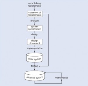
• Design begins with a system specification, produces design documents and provides a detailed description of
how a system should be constructed.
• Implementation is the construction of a computer system according to a given design document and taking
into account the environment in which the system will be operating (e.g., specific hardware or software
available for the development). Implementation may be staged, usually with an initial system that can be
validated and tested before a final system is released for use.
• Testing compares the implemented system against the design documents and requirements specification and
produces an acceptance report or, more usually, a list of errors and bugs that require a review of the analysis,
design and implementation processes to correct (testing is usually the task that leads to the waterfall model
iterating through the life cycle).
• Maintenance involves dealing with changes in the requirements or the implementation environment, bug
fixing or porting of the system to new environments (e.g., migrating a system from a standalone PC to a
UNIX workstation or a networked environment). Since maintenance involves the analysis of the changes
required, design of a solution, implementation and testing of that solution over the lifetime of a maintained
software system, the waterfall life cycle will be repeatedly revisited.
Database Life Cycle
We can use the waterfall cycle as the basis for a model of database development that incorporates three assumptions:
1. We can separate the development of a database – that is, specification and creation of a schema to define
data in a database – from the user processes that make use of the database.
2. We can use the three-schema architecture as a basis for distinguishing the activities associated with a
schema.
3. We can represent the constraints to enforce the semantics of the data once within a database, rather than
within every user process that uses the data.
Using these assumptions and Figure 13.2, we can see that this diagram represents a model of the activities and their out-
puts for database development. It is applicable to any class of DBMS, not just a relational approach.
Database application development is the process of obtaining real-world requirements, analyzing requirements, design-
ing the data and functions of the system, and then implementing the operations in the system.
Requirements Gathering
The first step is requirements gathering. During this step, the database designers have to interview the customers (database
users) to understand the proposed system and obtain and document the data and functional requirements. The result of
this step is a document that includes the detailed requirements provided by the users.
Establishing requirements involves consultation with, and agreement among, all the users as to what persistent data they
want to store along with an agreement as to the meaning and interpretation of the data elements. The data administra-
tor plays a key role in this process as they overview the business, legal and ethical issues within the organization that
impact on the data requirements.
The data requirements document is used to confirm the understanding of requirements with users. To make sure that it is
easily understood, it should not be overly formal or highly encoded. The document should give a concise summary of all
CHAPTER 13 DATABASE DEVELOPMENT PROCESS • 75
THIS TEXTBOOK IS AVAILABLE FOR FREE AT OPEN.BCCAMPUS.CA
Figure 13.2. A waterfall model of the activities and their outputs for
database development.
users’ requirements – not just a collection of individuals’ requirements – as the intention is to develop a single shared
database.
The requirements should not describe how the data is to be processed, but rather what the data items are, what attributes
they have, what constraints apply and the relationships that hold between the data items.
Analysis
Data analysis begins with the statement of data requirements and then produces a conceptual data model. The aim of
analysis is to obtain a detailed description of the data that will suit user requirements so that both high and low level
properties of data and their use are dealt with. These include properties such as the possible range of values that can be
permitted for attributes (e.g., in the school database example, the student course code, course title and credit points).
The conceptual data model provides a shared, formal representation of what is being communicated between clients
and developers during database development – it is focused on the data in a database, irrespective of the eventual use of
that data in user processes or implementation of the data in specific computer environments. Therefore, a conceptual
data model is concerned with the meaning and structure of data, but not with the details affecting how they are imple-
mented.
The conceptual data model then is a formal representation of what data a database should contain and the constraints
the data must satisfy. This should be expressed in terms that are independent of how the model may be implemented. As
a result, analysis focuses on the questions, “What is required?” not “How is it achieved?”
76 •
THIS TEXTBOOK IS AVAILABLE FOR FREE AT OPEN.BCCAMPUS.CA
Logical Design
Database design starts with a conceptual data model and produces a specification of a logical schema; this will determine
the specific type of database system (network, relational, object-oriented) that is required. The relational representation
is still independent of any specific DBMS; it is another conceptual data model.
We can use a relational representation of the conceptual data model as input to the logical design process. The output of
this stage is a detailed relational specification, the logical schema, of all the tables and constraints needed to satisfy the
description of the data in the conceptual data model. It is during this design activity that choices are made as to which
tables are most appropriate for representing the data in a database. These choices must take into account various design
criteria including, for example, flexibility for change, control of duplication and how best to represent the constraints. It
is the tables defined by the logical schema that determine what data are stored and how they may be manipulated in the
database.
Database designers familiar with relational databases and SQL might be tempted to go directly to implementation after
they have produced a conceptual data model. However, such a direct transformation of the relational representation to
SQL tables does not necessarily result in a database that has all the desirable properties: completeness, integrity, flex-
ibility, efficiency and usability. A good conceptual data model is an essential first step towards a database with these
properties, but that does not mean that the direct transformation to SQL tables automatically produces a good database.
This first step will accurately represent the tables and constraints needed to satisfy the conceptual data model descrip-
tion, and so will satisfy the completeness and integrity requirements, but it may be inflexible or offer poor usability. The
first design is then flexed to improve the quality of the database design. Flexing is a term that is intended to capture the
simultaneous ideas of bending something for a different purpose and weakening aspects of it as it is bent.
Figure 13.3 summarizes the iterative (repeated) steps involved in database design, based on the overview given. Its main
purpose is to distinguish the general issue of what tables should be used from the detailed definition of the constituent
parts of each table – these tables are considered one at a time, although they are not independent of each other. Each
iteration that involves a revision of the tables would lead to a new design; collectively they are usually referred to as
second-cut designs, even if the process iterates for more than a single loop.
Figure 13.3. A summary of the iterative steps involved in database
design.
First, for a given conceptual data model, it is not necessary that all the user requirements it represents be satisfied by
a single database. There can be various reasons for the development of more than one database, such as the need for
independent operation in different locations or departmental control over “their” data. However, if the collection of
CHAPTER 13 DATABASE DEVELOPMENT PROCESS • 77
THIS TEXTBOOK IS AVAILABLE FOR FREE AT OPEN.BCCAMPUS.CA
databases contains duplicated data and users need to access data in more than one database, then there are possible rea-
sons that one database can satisfy multiple requirements, or issues related to data replication and distribution need to
be examined.
Second, one of the assumptions about database development is that we can separate the development of a database from
the development of user processes that make use of it. This is based on the expectation that, once a database has been
implemented, all data required by currently identified user processes have been defined and can be accessed; but we
also require flexibility to allow us to meet future requirements changes. In developing a database for some applications,
it may be possible to predict the common requests that will be presented to the database and so we can optimize our
design for the most common requests.
Third, at a detailed level, many aspects of database design and implementation depend on the particular DBMS being
used. If the choice of DBMS is fixed or made prior to the design task, that choice can be used to determine design crite-
ria rather than waiting until implementation. That is, it is possible to incorporate design decisions for a specific DBMS
rather than produce a generic design and then tailor it to the DBMS during implementation.
It is not uncommon to find that a single design cannot simultaneously satisfy all the properties of a good database. So it
is important that the designer has prioritized these properties (usually using information from the requirements speci-
fication); for example, to decide if integrity is more important than efficiency and whether usability is more important
than flexibility in a given development.
At the end of our design stage, the logical schema will be specified by SQL data definition language (DDL) statements,
which describe the database that needs to be implemented to meet the user requirements.
Implementation
Implementation involves the construction of a database according to the specification of a logical schema. This will
include the specification of an appropriate storage schema, security enforcement, external schema and so on. Imple-
mentation is heavily influenced by the choice of available DBMSs, database tools and operating environment. There are
additional tasks beyond simply creating a database schema and implementing the constraints – data must be entered
into the tables, issues relating to the users and user processes need to be addressed, and the management activities asso-
ciated with wider aspects of corporate data management need to be supported. In keeping with the DBMS approach, we
want as many of these concerns as possible to be addressed within the DBMS. We look at some of these concerns briefly
now.
In practice, implementation of the logical schema in a given DBMS requires a very detailed knowledge of the specific
features and facilities that the DBMS has to offer. In an ideal world, and in keeping with good software engineering prac-
tice, the first stage of implementation would involve matching the design requirements with the best available imple-
menting tools and then using those tools for the implementation. In database terms, this might involve choosing vendor
products with DBMS and SQL variants most suited to the database we need to implement. However, we don’t live in
an ideal world and more often than not, hardware choice and decisions regarding the DBMS will have been made well
in advance of consideration of the database design. Consequently, implementation can involve additional flexing of the
design to overcome any software or hardware limitations.
Realizing the Design
After the logical design has been created, we need our database to be created according to the definitions we have pro-
duced. For an implementation with a relational DBMS, this will probably involve the use of SQL to create tables and
78 •
THIS TEXTBOOK IS AVAILABLE FOR FREE AT OPEN.BCCAMPUS.CA
constraints that satisfy the logical schema description and the choice of appropriate storage schema (if the DBMS per-
mits that level of control).
One way to achieve this is to write the appropriate SQL DDL statements into a file that can be executed by a DBMS so
that there is an independent record, a text file, of the SQL statements defining the database. Another method is to work
interactively using a database tool like SQL Server Management Studio or Microsoft Access. Whatever mechanism is
used to implement the logical schema, the result is that a database, with tables and constraints, is defined but will con-
tain no data for the user processes.
Populating the Database
After a database has been created, there are two ways of populating the tables – either from existing data or through the
use of the user applications developed for the database.
For some tables, there may be existing data from another database or data files. For example, in establishing a database
for a hospital, you would expect that there are already some records of all the staff that have to be included in the data-
base. Data might also be brought in from an outside agency (address lists are frequently brought in from external com-
panies) or produced during a large data entry task (converting hard-copy manual records into computer files can be
done by a data entry agency). In such situations, the simplest approach to populate the database is to use the import and
export facilities found in the DBMS.
Facilities to import and export data in various standard formats are usually available (these functions are also known in
some systems as loading and unloading data). Importing enables a file of data to be copied directly into a table. When
data are held in a file format that is not appropriate for using the import function, then it is necessary to prepare an
application program that reads in the old data, transforms them as necessary and then inserts them into the database
using SQL code specifically produced for that purpose. The transfer of large quantities of existing data into a database is
referred to as a bulk load. Bulk loading of data may involve very large quantities of data being loaded, one table at a time
so you may find that there are DBMS facilities to postpone constraint checking until the end of the bulk loading.
Guidelines for Developing an ER Diagram
Note: These are general guidelines that will assist in developing a strong basis for the actual database design (the logical
model).
1. Document all entities discovered during the information-gathering stage.
2. Document all attributes that belong to each entity. Select candidate and primary keys. Ensure that all non-
key attributes for each entity are full-functionally dependent on the primary key.
3. Develop an initial ER diagram and review it with appropriate personnel. (Remember that this is an
iterative process.)
4. Create new entities (tables) for multivalued attributes and repeating groups. Incorporate these new entities
(tables) in the ER diagram. Review with appropriate personnel.
5. Verify ER modeling by normalizing tables.
Key Terms
analysis: starts by considering the statement of requirements and finishes by producing a system specification
CHAPTER 13 DATABASE DEVELOPMENT PROCESS • 79
THIS TEXTBOOK IS AVAILABLE FOR FREE AT OPEN.BCCAMPUS.CA
bulk load: the transfer of large quantities of existing data into a database
data requirements document: used to confirm the understanding of requirements with the user
design: begins with a system specification, produces design documents and provides a detailed description of
how a system should be constructed
establishing requirements: involves consultation with, and agreement among, stakeholders as to what they
want from a system; expressed as a statement of requirements
flexing: a term that captures the simultaneous ideas of bending something for a different purpose and weakening
aspects of it as it is bent
implementation: the construction of a computer system according to a given design document
maintenance: involves dealing with changes in the requirements or the implementation environment, bug fix-
ing or porting of the system to new environments
requirements gathering: a process during which the database designer interviews the database user to under-
stand the proposed system and obtain and document the data and functional requirements
second-cut designs: the collection of iterations that each involves a revision of the tables that lead to a new
design
software development life cycle (SDLC): the series of steps involved in the database development process
testing: compares the implemented system against the design documents and requirements specification and
produces an acceptance report
waterfall model: shows the database development process as a strict sequence of steps where the output of one
step is the input to the next
waterfall process: a means of identifying the tasks required for database development, together with the input
and output for each activity (see waterfall model)
Exercises
1. Describe the waterfall model. List the steps.
2. What does the acronym SDLC mean, and what does an SDLC portray?
3. What needs to be modified in the waterfall model to accommodate database design?
4. Provide the iterative steps involved in database design.
80 •
THIS TEXTBOOK IS AVAILABLE FOR FREE AT OPEN.BCCAMPUS.CA
Attribution
This chapter of Database Design (including all images, except as otherwise noted) is a derivative copy of The Database
Development Life Cycle by the Open University licensed under Creative Commons Attribution-NonCommercial-
ShareAlike 3.0 License.
The following material was written by Adrienne Watt:
1. Key Terms
2. Exercises
CHAPTER 13 DATABASE DEVELOPMENT PROCESS • 81
THIS TEXTBOOK IS AVAILABLE FOR FREE AT OPEN.BCCAMPUS.CA
Chapter 14 Database Users Adrienne Watt
End Users
End users are the people whose jobs require access to a database for querying, updating and generating reports.
Application user
The application user is someone who accesses an existing application program to perform daily tasks.
Sophisticated user
Sophisticated users are those who have their own way of accessing the database. This means they do not use the applica-
tion program provided in the system. Instead, they might define their own application or describe their need directly by
using query languages. These specialized users maintain their personal databases by using ready-made program pack-
ages that provide easy-to-use menu driven commands, such as MS Access.
Application Programmers
These users implement specific application programs to access the stored data. They must be familiar with the DBMSs
to accomplish their task.
Database Administrators (DBA)
This may be one person or a group of people in an organization responsible for authorizing access to the database, mon-
itoring its use and managing all of the resources to support the use of the entire database system.
Key Terms
application programmer: user who implements specific application programs to access the stored data
application user: accesses an existing application program to perform daily tasks.
database administrator (DBA): responsible for authorizing access to the database, monitoring its use and man-
aging all the resources to support the use of the entire database system
end user: people whose jobs require access to a database for querying, updating and generating reports
sophisticated user: those who use other methods, other than the application program, to access the database
There are no exercises provided for this chapter.
82
Chapter 15 SQL Structured Query Language Adrienne Watt & Nelson Eng
Structured Query Language (SQL) is a database language designed for managing data held in a relational database man-
agement system. SQL was initially developed by IBM in the early 1970s (Date 1986). The initial version, called SEQUEL
(Structured English Query Language), was designed to manipulate and retrieve data stored in IBM’s quasi-relational
database management system, System R. Then in the late 1970s, Relational Software Inc., which is now Oracle Corpo-
ration, introduced the first commercially available implementation of SQL, Oracle V2 for VAX computers.
Many of the currently available relational DBMSs, such as Oracle Database, Microsoft SQL Server (shown in Figure
15.1), MySQL, IBM DB2, IBM Informix and Microsoft Access, use SQL.
Figure 15.1. Example of Microsoft SQL Server, by A. Watt.
In a DBMS, the SQL database language is used to:
• Create the database and table structures
• Perform basic data management chores (add, delete and modify)
• Perform complex queries to transform raw data into useful information
In this chapter, we will focus on using SQL to create the database and table structures, mainly using SQL as a data def-
inition language (DDL). In Chapter 16, we will use SQL as a data manipulation language (DML) to insert, delete, select
and update data within the database tables.
83
Create Database
The major SQL DDL statements are CREATE DATABASE and CREATE/DROP/ALTER TABLE. The SQL statement
CREATE is used to create the database and table structures.
Example: CREATE DATABASE SW
A new database named SW is created by the SQL statement CREATE DATABASE SW. Once the database is created, the
next step is to create the database tables.
The general format for the CREATE TABLE command is:
CREATE TABLE <tablename>
(
ColumnName, Datatype, Optional Column Constraint,
ColumnName, Datatype, Optional Column Constraint,
Optional table Constraints
);
Tablename is the name of the database table such as Employee. Each field in the CREATE TABLE has three parts (see
above):
1. ColumnName
2. Data type
3. Optional Column Constraint
ColumnName
The ColumnName must be unique within the table. Some examples of ColumnNames are FirstName and LastName.
Data Type
The data type, as described below, must be a system data type or a user-defined data type. Many of the data types have a
size such as CHAR(35) or Numeric(8,2).
Bit –Integer data with either a 1 or 0 value
Int –Integer (whole number) data from -2^31 (-2,147,483,648) through 2^31 – 1 (2,147,483,647)
Smallint –Integer data from 2^15 (-32,768) through 2^15 – 1 (32,767)
Tinyint –Integer data from 0 through 255
Decimal –Fixed precision and scale numeric data from -10^38 -1 through 10^38
Numeric –A synonym for decimal
84 •
THIS TEXTBOOK IS AVAILABLE FOR FREE AT OPEN.BCCAMPUS.CA
Timestamp –A database-wide unique number
Uniqueidentifier –A globally unique identifier (GUID)
Money - Monetary data values from -2^63 (-922,337,203,685,477.5808) through 2^63 – 1 (+922,337,203,685,477.5807),
with accuracy to one-ten-thousandth of a monetary unit
Smallmoney –Monetary data values from -214,748.3648 through +214,748.3647, with accuracy to one-ten-thou-
sandth of a monetary unit
Float –Floating precision number data from -1.79E + 308 through 1.79E + 308
Real –Floating precision number data from -3.40E + 38 through 3.40E + 38
Datetime –Date and time data from January 1, 1753, to December 31, 9999, with an accuracy of one-three-hundredths
of a second, or 3.33 milliseconds
Smalldatetime –Date and time data from January 1, 1900, through June 6, 2079, with an accuracy of one minute
Char –Fixed-length non-Unicode character data with a maximum length of 8,000 characters
Varchar –Variable-length non-Unicode data with a maximum of 8,000 characters
Text –Variable-length non-Unicode data with a maximum length of 2^31 – 1 (2,147,483,647) characters
Binary –Fixed-length binary data with a maximum length of 8,000 bytes
Varbinary –Variable-length binary data with a maximum length of 8,000 bytes
Image – Variable-length binary data with a maximum length of 2^31 – 1 (2,147,483,647) bytes
Optional Column Constraints
The Optional ColumnConstraints are NULL, NOT NULL, UNIQUE, PRIMARY KEY and DEFAULT, used to initialize
a value for a new record. The column constraint NULL indicates that null values are allowed, which means that a row
can be created without a value for this column. The column constraint NOT NULL indicates that a value must be sup-
plied when a new row is created.
To illustrate, we will use the SQL statement CREATE TABLE EMPLOYEES to create the employees table with 16 attrib-
utes or fields.
The first field is EmployeeNo with a field type of CHAR. For this field, the field length is 10 characters, and the user
cannot leave this field empty (NOT NULL).
Similarly, the second field is DepartmentName with a field type CHAR of length 30. After all the table columns are
defined, a table constraint, identified by the word CONSTRAINT, is used to create the primary key:
CONSTRAINT EmployeePK PRIMARY KEY(EmployeeNo)
CHAPTER 15 SQL STRUCTURED QUERY LANGUAGE • 85
THIS TEXTBOOK IS AVAILABLE FOR FREE AT OPEN.BCCAMPUS.CA
USE SW
CREATE TABLE EMPLOYEES
(
EmployeeNo CHAR(10) NOT NULL UNIQUE,
DepartmentName CHAR(30) NOT NULL DEFAULT “Human Resources”,
FirstName CHAR(25) NOT NULL,
LastName CHAR(25) NOT NULL,
Category CHAR(20) NOT NULL,
HourlyRate CURRENCY NOT NULL,
TimeCard LOGICAL NOT NULL,
HourlySalaried CHAR(1) NOT NULL,
EmpType CHAR(1) NOT NULL,
Terminated LOGICAL NOT NULL,
ExemptCode CHAR(2) NOT NULL,
Supervisor LOGICAL NOT NULL,
SupervisorName CHAR(50) NOT NULL,
BirthDate DATE NOT NULL,
CollegeDegree CHAR(5) NOT NULL,
CONSTRAINT Employee_PK PRIMARY KEY(EmployeeNo
);
We will discuss the constraint property further later in this chapter.
Likewise, we can create a Department table, a Project table and an Assignment table using the CREATE TABLE SQL
DDL command as shown in the below example.
USE SW
CREATE TABLE DEPARTMENT
(
DepartmentName Char(35) NOT NULL,
BudgetCode Char(30) NOT NULL,
OfficeNumber Char(15) NOT NULL,
Phone Char(15) NOT NULL,
CONSTRAINT DEPARTMENT_PK PRIMARY KEY(DepartmentName)
);
In this example, a project table is created with seven fields: ProjectID, ProjectName, Department, MaxHours, StartDate,
and EndDate.
In this last example, an assignment table is created with three fields: ProjectID, EmployeeNumber, and HoursWorked.
The assignment table is used to record who (EmployeeNumber) and how much time(HoursWorked) an employee
worked on the particular project(ProjectID).
86 •
THIS TEXTBOOK IS AVAILABLE FOR FREE AT OPEN.BCCAMPUS.CA
USE SW
CREATE TABLE PROJECT
(
ProjectID Int NOT NULL IDENTITY (1000,100),
ProjectName Char(50) NOT NULL,
Department Char(35) NOT NULL,
MaxHours Numeric(8,2) NOT NULL DEFAULT 100,
StartDate DateTime NULL,
EndDate DateTime NULL,
CONSTRAINT ASSIGNMENT_PK PRIMARY KEY(ProjectID)
);
USE SW
CREATE TABLE ASSIGNMENT
(
ProjectID Int NOT NULL,
EmployeeNumber Int NOT NULL,
HoursWorked Numeric(6,2) NULL,
);
Table Constraints
Table constraints are identified by the CONSTRAINT keyword and can be used to implement various constraints
described below.
IDENTITY constraint
We can use the optional column constraint IDENTITY to provide a unique, incremental value for that column. Identity
columns are often used with the PRIMARY KEY constraints to serve as the unique row identifier for the table. The
IDENTITY property can be assigned to a column with a tinyint, smallint, int, decimal or numeric data type. This con-
straint:
• Generates sequential numbers
• Does not enforce entity integrity
• Only one column can have the IDENTITY property
• Must be defined as an integer, numeric or decimal data type
• Cannot update a column with the IDENTITY property
• Cannot contain NULL values
• Cannot bind defaults and default constraints to the column
For IDENTITY[(seed, increment)]
CHAPTER 15 SQL STRUCTURED QUERY LANGUAGE • 87
THIS TEXTBOOK IS AVAILABLE FOR FREE AT OPEN.BCCAMPUS.CA
• Seed – the initial value of the identity column
• Increment – the value to add to the last increment column
We will use another database example to further illustrate the SQL DDL statements by creating the table tblHotel in this
HOTEL database.
CREATE TABLE tblHotel
(
HotelNo Int IDENTITY (1,1),
Name Char(50) NOT NULL,
Address Char(50) NULL,
City Char(25) NULL,
)
UNIQUE constraint
The UNIQUE constraint prevents duplicate values from being entered into a column.
• Both PK and UNIQUE constraints are used to enforce entity integrity.
• Multiple UNIQUE constraints can be defined for a table.
• When a UNIQUE constraint is added to an existing table, the existing data is always validated.
• A UNIQUE constraint can be placed on columns that accept nulls. Only one row can be NULL.
• A UNIQUE constraint automatically creates a unique index on the selected column.
This is the general syntax for the UNIQUE constraint:
[CONSTRAINT constraint_name]
UNIQUE [CLUSTERED | NONCLUSTERED]
(col_name [, col_name2 […, col_name16]])
[ON segment_name]
This is an examle using the UNIQUE constraint.
CREATE TABLE EMPLOYEES
(
EmployeeNo CHAR(10) NOT NULL UNIQUE,
)
FOREIGN KEY constraint
The FOREIGN KEY (FK) constraint defines a column, or combination of columns, whose values match the PRIMARY
KEY (PK) of another table.
88 •
THIS TEXTBOOK IS AVAILABLE FOR FREE AT OPEN.BCCAMPUS.CA
• Values in an FK are automatically updated when the PK values in the associated table are updated/changed.
• FK constraints must reference PK or the UNIQUE constraint of another table.
• The number of columns for FK must be same as PK or UNIQUE constraint.
• If the WITH NOCHECK option is used, the FK constraint will not validate existing data in a table.
• No index is created on the columns that participate in an FK constraint.
This is the general syntax for the FOREIGN KEY constraint:
[CONSTRAINT constraint_name]
[FOREIGN KEY (col_name [, col_name2 […, col_name16]])]
REFERENCES [owner.]ref_table [(ref_col [, ref_col2 […, ref_col16]])]
In this example, the field HotelNo in the tblRoom table is a FK to the field HotelNo in the tblHotel table shown previ-
ously.
USE HOTEL
GO
CREATE TABLE tblRoom
(
HotelNo Int NOT NULL ,
RoomNo Int NOT NULL,
Type Char(50) NULL,
Price Money NULL,
PRIMARY KEY (HotelNo, RoomNo),
FOREIGN KEY (HotelNo) REFERENCES tblHotel
)
CHECK constraint
The CHECK constraint restricts values that can be entered into a table.
• It can contain search conditions similar to a WHERE clause.
• It can reference columns in the same table.
• The data validation rule for a CHECK constraint must evaluate to a boolean expression.
• It can be defined for a column that has a rule bound to it.
This is the general syntax for the CHECK constraint:
[CONSTRAINT constraint_name]
CHECK [NOT FOR REPLICATION] (expression)
In this example, the Type field is restricted to have only the types ‘Single’, ‘Double’, ‘Suite’ or ‘Executive’.
CHAPTER 15 SQL STRUCTURED QUERY LANGUAGE • 89
THIS TEXTBOOK IS AVAILABLE FOR FREE AT OPEN.BCCAMPUS.CA
USE HOTEL
GO
CREATE TABLE tblRoom
(
HotelNo Int NOT NULL,
RoomNo Int NOT NULL,
Type Char(50) NULL,
Price Money NULL,
PRIMARY KEY (HotelNo, RoomNo),
FOREIGN KEY (HotelNo) REFERENCES tblHotel
CONSTRAINT Valid_Type
CHECK (Type IN (‘Single’, ‘Double’, ‘Suite’, ‘Executive’))
)
In this second example, the employee hire date should be before January 1, 2004, or have a salary limit of $300,000.
GO
CREATE TABLE SALESREPS
(
Empl_num Int Not Null
CHECK (Empl_num BETWEEN 101 and 199),
Name Char (15),
Age Int CHECK (Age >= 21),
Quota Money CHECK (Quota >= 0.0),
HireDate DateTime,
CONSTRAINT QuotaCap CHECK ((HireDate < “01-01-2004”) OR (Quota <=300000))
)
DEFAULT constraint
The DEFAULT constraint is used to supply a value that is automatically added for a column if the user does not supply
one.
• A column can have only one DEFAULT.
• The DEFAULT constraint cannot be used on columns with a timestamp data type or identity property.
• DEFAULT constraints are automatically bound to a column when they are created.
The general syntax for the DEFAULT constraint is:
This example sets the default for the city field to ‘Vancouver’.
90 •
THIS TEXTBOOK IS AVAILABLE FOR FREE AT OPEN.BCCAMPUS.CA
[CONSTRAINT constraint_name]
DEFAULT {constant_expression | niladic-function | NULL}
[FOR col_name]
USE HOTEL
ALTER TABLE tblHotel
Add CONSTRAINT df_city DEFAULT ‘Vancouver’ FOR City
User Defined Types
User defined types are always based on system-supplied data type. They can enforce data integrity and they allow nulls.
To create a user-defined data type in SQL Server, choose types under “Programmability” in your database. Next, right
click and choose ‘New’ –>‘User-defined data type’ or execute the sp_addtype system stored procedure. After this, type:
sp_addtype ssn, ‘varchar(11)’, ‘NOT NULL’
This will add a new user-defined data type called SIN with nine characters.
In this example, the field EmployeeSIN uses the user-defined data type SIN.
CREATE TABLE SINTable
(
EmployeeID INT Primary Key,
EmployeeSIN SIN,
CONSTRAINT CheckSIN
CHECK (EmployeeSIN LIKE
‘ [0-9][0-9][0-9] – [0-9][0-9] [0-9] – [0-9][0-9][0-9] ‘)
)
ALTER TABLE
You can use ALTER TABLE statements to add and drop constraints.
• ALTER TABLE allows columns to be removed.
• When a constraint is added, all existing data are verified for violations.
In this example, we use the ALTER TABLE statement to the IDENTITY property to a ColumnName field.
Use the ALTER TABLE statement to add a column with the IDENTITY property such as ALTER TABLE TableName.
CHAPTER 15 SQL STRUCTURED QUERY LANGUAGE • 91
THIS TEXTBOOK IS AVAILABLE FOR FREE AT OPEN.BCCAMPUS.CA
USE HOTEL
GO
ALTER TABLE tblHotel
ADD CONSTRAINT unqName UNIQUE (Name)
ADD
ColumnName int IDENTITY(seed, increment)
DROP TABLE
The DROP TABLE will remove a table from the database. Make sure you have the correct database selected.
DROP TABLE tblHotel
Executing the above SQL DROP TABLE statement will remove the table tblHotel from the database.
Key Terms
DDL: abbreviation for data definition language
DML: abbreviation for data manipulation language
SEQUEL: acronym for Structured English Query Language; designed to manipulate and retrieve data stored in
IBM’s quasi-relational database management system, System R
Structured Query Language (SQL): a database language designed for managing data held in a relational data-
base management system
Exercises
1. Using the information for the Chapter 9 exercise, implement the schema using Transact SQL (show
SQL statements for each table). Implement the constraints as well.
2. Create the table shown here in SQL Server and show the statements you used.
Table: Employee
ATTRIBUTE (FIELD) NAME DATA DECLARATION
EMP_NUM CHAR(3)
EMP_LNAME VARCHAR(15)
EMP_FNAME VARCHAR(15)
92 •
THIS TEXTBOOK IS AVAILABLE FOR FREE AT OPEN.BCCAMPUS.CA
EMP_INITIAL CHAR(1)
EMP_HIREDATE DATE
JOB_CODE CHAR(3)
3. Having created the table structure in question 2, write the SQL code to enter the rows for the table
shown in Figure 15.1.
Figure 15.2. Employee table with data for questions 4-10, by A. Watt.
Use Figure 15.2 to answer questions 4 to 10.
4. Write the SQL code to change the job code to 501 for the person whose personnel number is 107.
After you have completed the task, examine the results, and then reset the job code to its original
value.
5. Assuming that the data shown in the Employee table have been entered, write the SQL code that
lists all attributes for a job code of 502.
6. Write the SQL code to delete the row for the person named William Smithfield, who was hired on
June 22, 2004, and whose job code classification is 500. (Hint: Use logical operators to include all the
information given in this problem.)
7. Add the attributes EMP_PCT and PROJ_NUM to the Employee table. The EMP_PCT is the bonus
percentage to be paid to each employee.
8. Using a single command, write the SQL code that will enter the project number (PROJ_NUM) = 18
for all employees whose job classification ( JOB_CODE) is 500.
9. Using a single command, write the SQL code that will enter the project number (PROJ_NUM) = 25
for all employees whose job classification ( JOB_CODE) is 502 or higher.
10. Write the SQL code that will change the PROJ_NUM to 14 for those employees who were hired
before January 1, 1994, and whose job code is at least 501. (You may assume that the table will be
restored to its original condition preceding this question.)
Also see Appendix C: SQL Lab with Solution
References
Date, C.J. Relational Database Selected Writings. Reading: Mass: Addison-Wesley Publishing Company Inc., 1986, p.
269-311.
CHAPTER 15 SQL STRUCTURED QUERY LANGUAGE • 93
THIS TEXTBOOK IS AVAILABLE FOR FREE AT OPEN.BCCAMPUS.CA
Chapter 16 SQL Data Manipulation Language Adrienne Watt & Nelson Eng
The SQL data manipulation language (DML) is used to query and modify database data. In this chapter, we will
describe how to use the SELECT, INSERT, UPDATE, and DELETE SQL DML command statements, defined below.
• SELECT – to query data in the database
• INSERT – to insert data into a table
• UPDATE – to update data in a table
• DELETE – to delete data from a table
In the SQL DML statement:
• Each clause in a statement should begin on a new line.
• The beginning of each clause should line up with the beginning of other clauses.
• If a clause has several parts, they should appear on separate lines and be indented under the start of the clause
to show the relationship.
• Upper case letters are used to represent reserved words.
• Lower case letters are used to represent user-defined words.
SELECT Statement
The SELECT statement, or command, allows the user to extract data from tables, based on specific criteria. It is
processed according to the following sequence:
SELECT DISTINCT item(s)
FROM table(s)
WHERE predicate
GROUP BY field(s)
ORDER BY fields
We can use the SELECT statement to generate an employee phone list from the Employees table as follows:
SELECT FirstName, LastName, phone
FROM Employees
ORDER BY LastName
This action will display employee’s last name, first name, and phone number from the Employees table, seen in Table
16.1.
Last Name First Name Phone Number
Hagans Jim 604-232-3232
Wong Bruce 604-244-2322
94
Table 16.1. Employees table.
In this next example, we will use a Publishers table (Table 16.2). (You will notice that Canada is mispelled in the Publisher
Country field for Example Publishing and ABC Publishing. To correct mispelling, use the UPDATE statement to stan-
dardize the country field to Canada – see UPDATE statement later in this chapter.)
Publisher Name Publisher City Publisher Province Publisher Country
Acme Publishing Vancouver BC Canada
Example Publishing Edmonton AB Cnada
ABC Publishing Toronto ON Canda
Table 16.2. Publishers table.
If you add the publisher’s name and city, you would use the SELECT statement followed by the fields name separated by
a comma:
SELECT PubName, city
FROM Publishers
This action will display the publisher’s name and city from the Publishers table.
If you just want the publisher’s name under the display name city, you would use the SELECT statement with no comma
separating pub_name and city:
SELECT PubName city
FROM Publishers
Performing this action will display only the pub_name from the Publishers table with a “city” heading. If you do not
include the comma, SQL Server assumes you want a new column name for pub_name.
SELECT statement with WHERE criteria
Sometimes you might want to focus on a portion of the Publishers table, such as only publishers that are in Vancouver.
In this situation, you would use the SELECT statement with the WHERE criterion, i.e., WHERE city = ‘Vancouver’.
These first two examples illustrate how to limit record selection with the WHERE criterion using BETWEEN. Each of
these examples give the same results for store items with between 20 and 50 items in stock.
Example #1 uses the quantity, qty BETWEEN 20 and 50.
SELECT StorID, qty, TitleID
FROM Sales
WHERE qty BETWEEN 20 and 50 (includes the 20 and 50)
CHAPTER 16 SQL DATA MANIPULATION LANGUAGE • 95
THIS TEXTBOOK IS AVAILABLE FOR FREE AT OPEN.BCCAMPUS.CA
Example #2, on the other hand, uses qty >=20 and qty <=50 .
SELECT StorID, qty, TitleID
FROM Sales
WHERE qty >= 20 and qty <= 50
Example #3 illustrates how to limit record selection with the WHERE criterion using NOT BETWEEN.
SELECT StorID, qty, TitleID
FROM Sales
WHERE qty NOT BETWEEN 20 and 50
The next two examples show two different ways to limit record selection with the WHERE criterion using IN, with each
yielding the same results.
Example #4 shows how to select records using province= as part of the WHERE statement.
SELECT *
FROM Publishers
WHERE province = ‘BC’ OR province = ‘AB’ OR province = ‘ON’
Example #5 select records using province IN as part of the WHERE statement.
SELECT *
FROM Publishers
WHERE province IN (‘BC’, ‘AB’, ‘ON’)
The final two examples illustrate how NULL and NOT NULL can be used to select records. For these examples, a
Books table (not shown) would be used that contains fields called Title, Quantity, and Price (of book). Each publisher has
a Books table that lists all of its books.
Example #6 uses NULL.
SELECT price, title
FROM Books
WHERE price IS NULL
Example #7 uses NOT NULL.
96 •
THIS TEXTBOOK IS AVAILABLE FOR FREE AT OPEN.BCCAMPUS.CA
SELECT price, title
FROM Books
WHERE price IS NOT NULL
Using wildcards in the LIKE clause
The LIKE keyword selects rows containing fields that match specified portions of character strings. LIKE is used with
char, varchar, text, datetime and smalldatetime data. A wildcard allows the user to match fields that contain certain let-
ters. For example, the wildcard province = ‘N%’ would give all provinces that start with the letter ‘N’. Table 16.3 shows
four ways to specify wildcards in the SELECT statement in regular express format.
%
Any string of zero or more characters
_
Any single character
[ ]
Any single character within the specified range (e.g., [a-f]) or set (e.g., [abcdef])
[^]
Any single character not within the specified range (e.g., [^a - f]) or set (e.g., [^abcdef])
Table 16.3. How to specify wildcards in the SELECT statement.
In example #1, LIKE ‘Mc%’ searches for all last names that begin with the letters “Mc” (e.g., McBadden).
SELECT LastName
FROM Employees
WHERE LastName LIKE ‘Mc%’
For example #2: LIKE ‘%inger’ searches for all last names that end with the letters “inger” (e.g., Ringer, Stringer).
SELECT LastName
FROM Employees
WHERE LastName LIKE ‘%inger’
In, example #3: LIKE ‘%en%’ searches for all last names that have the letters “en” (e.g., Bennett, Green, McBadden).
SELECT LastName
FROM Employees
WHERE LastName LIKE ‘%en%’
CHAPTER 16 SQL DATA MANIPULATION LANGUAGE • 97
THIS TEXTBOOK IS AVAILABLE FOR FREE AT OPEN.BCCAMPUS.CA
SELECT statement with ORDER BY clause
You use the ORDER BY clause to sort the records in the resulting list. Use ASC to sort the results in ascending order and
DESC to sort the results in descending order.
For example, with ASC:
SELECT *
FROM Employees
ORDER BY HireDate ASC
And with DESC:
SELECT *
FROM Books
ORDER BY type, price DESC
SELECT statement with GROUP BY clause
The GROUP BY clause is used to create one output row per each group and produces summary values for the selected
columns, as shown below.
SELECT type
FROM Books
GROUP BY type
Here is an example using the above statement.
SELECT type AS ‘Type’, MIN(price) AS ‘Minimum Price’
FROM Books
WHERE royalty > 10
GROUP BY type
If the SELECT statement includes a WHERE criterion where price is not null,
SELECT type, price
FROM Books
WHERE price is not null
then a statement with the GROUP BY clause would look like this:
98 •
THIS TEXTBOOK IS AVAILABLE FOR FREE AT OPEN.BCCAMPUS.CA
SELECT type AS ‘Type’, MIN(price) AS ‘Minimum Price’
FROM Books
WHERE price is not null
GROUP BY type
Using COUNT with GROUP BY
We can use COUNT to tally how many items are in a container. However, if we want to count different items into sep-
arate groups, such as marbles of varying colours, then we would use the COUNT function with the GROUP BY com-
mand.
The below SELECT statement illustrates how to count groups of data using the COUNT function with the GROUP BY
clause.
SELECT COUNT(*)
FROM Books
GROUP BY type
Using AVG and SUM with GROUP BY
We can use the AVG function to give us the average of any group, and SUM to give the total.
Example #1 uses the AVG FUNCTION with the GROUP BY type.
SELECT AVG(qty)
FROM Books
GROUP BY type
Example #2 uses the SUM function with the GROUP BY type.
SELECT SUM(qty)
FROM Books
GROUP BY type
Example #3 uses both the AVG and SUM functions with the GROUP BY type in the SELECT statement.
SELECT ‘Total Sales’ = SUM(qty), ‘Average Sales’ = AVG(qty), stor_id
FROM Sales
GROUP BY StorID ORDER BY ‘Total Sales’
CHAPTER 16 SQL DATA MANIPULATION LANGUAGE • 99
THIS TEXTBOOK IS AVAILABLE FOR FREE AT OPEN.BCCAMPUS.CA
Restricting rows with HAVING
The HAVING clause can be used to restrict rows. It is similar to the WHERE condition except HAVING can include the
aggregate function; the WHERE cannot do this.
The HAVING clause behaves like the WHERE clause, but is applicable to groups. In this example, we use the HAVING
clause to exclude the groups with the province ‘BC’.
SELECT au_fname AS ‘Author”s First Name’, province as ‘Province’
FROM Authors
GROUP BY au_fname, province
HAVING province <> ‘BC’
INSERT statement
The INSERT statement adds rows to a table. In addition,
• INSERT specifies the table or view that data will be inserted into.
• Column_list lists columns that will be affected by the INSERT.
• If a column is omitted, each value must be provided.
• If you are including columns, they can be listed in any order.
• VALUES specifies the data that you want to insert into the table. VALUES is required.
• Columns with the IDENTITY property should not be explicitly listed in the column_list or values_clause.
The syntax for the INSERT statement is:
INSERT [INTO] Table_name | view name [column_list]
DEFAULT VALUES | values_list | select statement
When inserting rows with the INSERT statement, these rules apply:
• Inserting an empty string (‘ ‘) into a varchar or text column inserts a single space.
• All char columns are right-padded to the defined length.
• All trailing spaces are removed from data inserted into varchar columns, except in strings that contain only
spaces. These strings are truncated to a single space.
• If an INSERT statement violates a constraint, default or rule, or if it is the wrong data type, the statement
fails and SQL Server displays an error message.
When you specify values for only some of the columns in the column_list, one of three things can happen to the columns
that have no values:
1. A default value is entered if the column has a DEFAULT constraint, if a default is bound to the column, or
if a default is bound to the underlying user-defined data type.
2. NULL is entered if the column allows NULLs and no default value exists for the column.
100 •
THIS TEXTBOOK IS AVAILABLE FOR FREE AT OPEN.BCCAMPUS.CA
3. An error message is displayed and the row is rejected if the column is defined as NOT NULL and
no default exists.
This example uses INSERT to add a record to the publisher’s Authors table.
INSERT INTO Authors
VALUES(‘555-093-467’, ‘Martin’, ‘April’, ‘281 555-5673’, ‘816 Market St.,’ , ‘Vancouver’, ‘BC’, ‘V7G3P4’, 0)
This following example illustrates how to insert a partial row into the Publishers table with a column list. The country
column had a default value of Canada so it does not require that you include it in your values.
INSERT INTO Publishers (PubID, PubName, city, province)
VALUES (‘9900’, ‘Acme Publishing’, ‘Vancouver’, ‘BC’)
To insert rows into a table with an IDENTITY column, follow the below example. Do not supply the value for the IDEN-
TITY nor the name of the column in the column list.
INSERT INTO jobs
VALUES (‘DBA’, 100, 175)
Inserting specific values into an IDENTITY column
By default, data cannot be inserted directly into an IDENTITY column; however, if a row is accidentally deleted, or there
are gaps in the IDENTITY column values, you can insert a row and specify the IDENTITY column value.
IDENTITY_INSERT option
To allow an insert with a specific identity value, the IDENTITY_INSERT option can be used as follows.
SET IDENTITY_INSERT jobs ON
INSERT INTO jobs (job_id, job_desc, min_lvl, max_lvl)
VALUES (19, ’DBA2’, 100, 175)
SET IDENTITY_INSERT jobs OFF
Inserting rows with a SELECT statement
We can sometimes create a small temporary table from a large table. For this, we can insert rows with a SELECT state-
ment. When using this command, there is no validation for uniqueness. Consequently, there may be many rows with the
same pub_id in the example below.
This example creates a smaller temporary Publishers table using the CREATE TABLE statement. Then the INSERT with
a SELECT statement is used to add records to this temporary Publishers table from the publis table.
CHAPTER 16 SQL DATA MANIPULATION LANGUAGE • 101
THIS TEXTBOOK IS AVAILABLE FOR FREE AT OPEN.BCCAMPUS.CA
CREATE TABLE dbo.tmpPublishers (
PubID char (4) NOT NULL ,
PubName varchar (40) NULL ,
city varchar (20) NULL ,
province char (2) NULL ,
country varchar (30) NULL DEFAULT (‘Canada’)
)
INSERT tmpPublishers
SELECT * FROM Publishers
In this example, we’re copying a subset of data.
INSERT tmpPublishers (pub_id, pub_name)
SELECT PubID, PubName
FROM Publishers
In this example, the publishers’ data are copied to the tmpPublishers table and the country column is set to Canada.
INSERT tmpPublishers (PubID, PubName, city, province, country)
SELECT PubID, PubName, city, province, ‘Canada’
FROM Publishers
UPDATE statement
The UPDATE statement changes data in existing rows either by adding new data or modifying existing data.
This example uses the UPDATE statement to standardize the country field to be Canada for all records in the Publishers
table.
UPDATE Publishers
SET country = ‘Canada’
This example increases the royalty amount by 10% for those royalty amounts between 10 and 20.
UPDATE roysched
SET royalty = royalty + (royalty * .10)
WHERE royalty BETWEEN 10 and 20
102 •
THIS TEXTBOOK IS AVAILABLE FOR FREE AT OPEN.BCCAMPUS.CA
Including subqueries in an UPDATE statement
The employees from the Employees table who were hired by the publisher in 2010 are given a promotion to the highest
job level for their job type. This is what the UPDATE statement would look like.
UPDATE Employees
SET job_lvl =
(SELECT max_lvl FROM jobs
WHERE employee.job_id = jobs.job_id)
WHERE DATEPART(year, employee.hire_date) = 2010
DELETE statement
The DELETE statement removes rows from a record set. DELETE names the table or view that holds the rows that will
be deleted and only one table or row may be listed at a time. WHERE is a standard WHERE clause that limits the dele-
tion to select records.
The DELETE syntax looks like this.
DELETE [FROM] {table_name | view_name }
[WHERE clause]
The rules for the DELETE statement are:
1. If you omit a WHERE clause, all rows in the table are removed (except for indexes, the table, constraints).
2. DELETE cannot be used with a view that has a FROM clause naming more than one table. (Delete can
affect only one base table at a time.)
What follows are three different DELETE statements that can be used.
1. Deleting all rows from a table.
DELETE
FROM Discounts
2. Deleting selected rows:
DELETE
FROM Sales
WHERE stor_id = ‘6380’
3. Deleting rows based on a value in a subquery:
CHAPTER 16 SQL DATA MANIPULATION LANGUAGE • 103
THIS TEXTBOOK IS AVAILABLE FOR FREE AT OPEN.BCCAMPUS.CA
DELETE FROM Sales
WHERE title_id IN
(SELECT title_id FROM Books WHERE type = ‘mod_cook’)
Built-in Functions
There are many built-in functions in SQL Server such as:
1. Aggregate: returns summary values
2. Conversion: transforms one data type to another
3. Date: displays information about dates and times
4. Mathematical: performs operations on numeric data
5. String: performs operations on character strings, binary data or expressions
6. System: returns a special piece of information from the database
7. Text and image: performs operations on text and image data
Below you will find detailed descriptions and examples for the first four functions.
Aggregate functions
Aggregate functions perform a calculation on a set of values and return a single, or summary, value. Table 16.4 lists these
functions.
FUNCTION DESCRIPTION
AVG Returns the average of all the values, or only the DISTINCT values, in the expression.
COUNT Returns the number of non-null values in the expression. When DISTINCT is specified, COUNT
finds the number of unique non-null values.
COUNT(*) Returns the number of rows. COUNT(*) takes no parameters and cannot be used with DISTINCT.
MAX Returns the maximum value in the expression. MAX can be used with numeric, character and
datetime columns, but not with bit columns. With character columns, MAX finds the highest value
in the collating sequence. MAX ignores any null values.
MIN Returns the minimum value in the expression. MIN can be used with numeric, character and
datetime columns, but not with bit columns. With character columns, MIN finds the value that is
lowest in the sort sequence. MIN ignores any null values.
SUM Returns the sum of all the values, or only the DISTINCT values, in the expression. SUM can be used
with numeric columns only.
Table 16.4 A list of aggregate functions and descriptions.
Below are examples of each of the aggregate functions listed in Table 16.4.
Example #1: AVG
Example #2: COUNT
104 •
THIS TEXTBOOK IS AVAILABLE FOR FREE AT OPEN.BCCAMPUS.CA
SELECT AVG (price) AS ‘Average Title Price’
FROM Books
SELECT COUNT(PubID) AS ‘Number of Publishers’
FROM Publishers
Example #3: COUNT
SELECT COUNT(province) AS ‘Number of Publishers’
FROM Publishers
Example #3: COUNT (*)
SELECT COUNT(*)
FROM Employees
WHERE job_lvl = 35
Example #4: MAX
SELECT MAX (HireDate)
FROM Employees
Example #5: MIN
SELECT MIN (price)
FROM Books
Example #6: SUM
SELECT SUM(discount) AS ‘Total Discounts’
FROM Discounts
Conversion function
The conversion function transforms one data type to another.
In the example below, a price that contains two 9s is converted into five characters. The syntax for this statement
is SELECT ‘The date is ‘ + CONVERT(varchar(12), getdate()).
CHAPTER 16 SQL DATA MANIPULATION LANGUAGE • 105
THIS TEXTBOOK IS AVAILABLE FOR FREE AT OPEN.BCCAMPUS.CA
SELECT CONVERT(int, 10.6496)
SELECT title_id, price
FROM Books
WHERE CONVERT(char(5), price) LIKE ‘%99%’
In this second example, the conversion function changes data to a data type with a different size.
SELECT title_id, CONVERT(char(4), ytd_sales) as ‘Sales’
FROM Books
WHERE type LIKE ‘%cook’
Date function
The date function produces a date by adding an interval to a specified date. The result is a datetime value equal to the
date plus the number of date parts. If the date parameter is a smalldatetime value, the result is also a smalldatetime value.
The DATEADD function is used to add and increment date values. The syntax for this function is DATEADD(datepart,
number, date).
SELECT DATEADD(day, 3, hire_date)
FROM Employees
In this example, the function DATEDIFF(datepart, date1, date2) is used.
This command returns the number of datepart “boundaries” crossed between two specified dates. The method of count-
ing crossed boundaries makes the result given by DATEDIFF consistent across all data types such as minutes, seconds,
and milliseconds.
SELECT DATEDIFF(day, HireDate, ‘Nov 30 1995′)
FROM Employees
For any particular date, we can examine any part of that date from the year to the millisecond.
The date parts (DATEPART) and abbreviations recognized by SQL Server, and the acceptable values are listed in Table
16.5.
DATE PART ABBREVIATION VALUES
Year yy 1753-9999
Quarter qq 1-4
Month mm 1-12
Day of year dy 1-366
Day dd 1-31
Week wk 1-53
106 •
THIS TEXTBOOK IS AVAILABLE FOR FREE AT OPEN.BCCAMPUS.CA
Weekday dw 1-7 (Sun.-Sat.)
Hour hh 0-23
Minute mi 0-59
Second ss 0-59
Millisecond ms 0-999
Table 16.5. Date part abbreviations and values.
Mathematical functions
Mathematical functions perform operations on numeric data. The following example lists the current price for each
book sold by the publisher and what they would be if all prices increased by 10%.
SELECT Price, (price * 1.1) AS ‘New Price’, title
FROM Books
SELECT ‘Square Root’ = SQRT(81)
SELECT ‘Rounded‘ = ROUND(4567.9876,2)
SELECT FLOOR (123.45)
Joining Tables
Joining two or more tables is the process of comparing the data in specified columns and using the comparison results
to form a new table from the rows that qualify. A join statement:
• Specifies a column from each table
• Compares the values in those columns row by row
• Combines rows with qualifying values into a new row
Although the comparison is usually for equality – values that match exactly – other types of joins can also be specified.
All the different joins such as inner, left (outer), right (outer), and cross join will be described below.
Inner join
An inner join connects two tables on a column with the same data type. Only the rows where the column values match
are returned; unmatched rows are discarded.
Example #1
SELECT jobs.job_id, job_desc
FROM jobs
INNER JOIN Employees ON employee.job_id = jobs.job_id
WHERE jobs.job_id < 7
CHAPTER 16 SQL DATA MANIPULATION LANGUAGE • 107
THIS TEXTBOOK IS AVAILABLE FOR FREE AT OPEN.BCCAMPUS.CA
Example #2
SELECT authors.au_fname, authors.au_lname, books.royalty, title
FROM authorsINNER JOIN titleauthor ON authors.au_id=titleauthor.au_id
INNER JOIN books ON titleauthor.title_id=books.title_id
GROUP BY authors.au_lname, authors.au_fname, title, title.royalty
ORDER BY authors.au_lname
Left outer join
A left outer join specifies that all left outer rows be returned. All rows from the left table that did not meet the condition
specified are included in the results set, and output columns from the other table are set to NULL.
This first example uses the new syntax for a left outer join.
SELECT publishers.pub_name, books.title
FROM Publishers
LEFT OUTER JOIN Books On publishers.pub_id = books.pub_id
This is an example of a left outer join using the old syntax.
SELECT publishers.pub_name, books.title
FROM Publishers, Books
WHERE publishers.pub_id *= books.pub_id
Right outer join
A right outer join includes, in its result set, all rows from the right table that did not meet the condition specified. Output
columns that correspond to the other table are set to NULL.
Below is an example using the new syntax for a right outer join.
SELECT titleauthor.title_id, authors.au_lname, authors.au_fname
FROM titleauthor
RIGHT OUTER JOIN authors ON titleauthor.au_id = authors.au_id
ORDERY BY au_lname
This second example show the old syntax used for a right outer join.
108 •
THIS TEXTBOOK IS AVAILABLE FOR FREE AT OPEN.BCCAMPUS.CA
SELECT titleauthor.title_id, authors.au_lname, authors.au_fname
FROM titleauthor, authors
WHERE titleauthor.au_id =* authors.au_id
ORDERY BY au_lname
Full outer join
A full outer join specifies that if a row from either table does not match the selection criteria, the row is included in the
result set, and its output columns that correspond to the other table are set to NULL.
Here is an example of a full outer join.
SELECT books.title, publishers.pub_name, publishers.province
FROM Publishers
FULL OUTER JOIN Books ON books.pub_id = publishers.pub_id
WHERE (publishers.province <> “BC” and publishers.province <> “ON”)
ORDER BY books.title_id
Cross join
A cross join is a product combining two tables. This join returns the same rows as if no WHERE clause were specified.
For example:
SELECT au_lname, pub_name,
FROM Authors CROSS JOIN Publishers
Key Terms
aggregate function: returns summary values
ASC: ascending order
conversion function: transforms one data type to another
cross join: a product combining two tables
date function: displays information about dates and times
DELETE statement: removes rows from a record set
CHAPTER 16 SQL DATA MANIPULATION LANGUAGE • 109
THIS TEXTBOOK IS AVAILABLE FOR FREE AT OPEN.BCCAMPUS.CA
DESC: descending order
full outer join: specifies that if a row from either table does not match the selection criteria
GROUP BY: used to create one output row per each group and produces summary values for the selected
columns
inner join: connects two tables on a column with the same data type
INSERT statement: adds rows to a table
left outer join: specifies that all left outer rows be returned
mathematical function: performs operations on numeric data
right outer join: includes all rows from the right table that did not meet the condition specified
SELECT statement: used to query data in the database
string function: performs operations on character strings, binary data or expressions
system function: returns a special piece of information from the database
text and image functions: performs operations on text and image data
UPDATE statement: changes data in existing rows either by adding new data or modifying existing data
wildcard: allows the user to match fields that contain certain letters.
Exercises
For questions 1 to 18 use the PUBS sample database created by Microsoft. To download the script to generate
this database please go to the following site: http://www.microsoft.com/en-ca/download/
details.aspx?id=23654.
1. Display a list of publication dates and titles (books) that were published in 2011.
2. Display a list of titles that have been categorized as either traditional or modern cooking. Use the
Books table.
3. Display all authors whose first names are five letters long.
4. Display from the Books table: type, price, pub_id, title about the books put out by each publisher.
Rename the column type with ”Book Category.” Sort by type (descending) and then price (ascending).
5. Display title_id, pubdate and pubdate plus three days, using the Books table.
6. Using the datediff and getdate function determine how much time has elapsed in months since the
books in the Books table were published.
7. List the title IDs and quantity of all books that sold more than 30 copies.
110 •
THIS TEXTBOOK IS AVAILABLE FOR FREE AT OPEN.BCCAMPUS.CA
8. Display a list of all last names of the authors who live in Ontario (ON) and the cities where they live.
9. Display all rows that contain a 60 in the payterms field. Use the Sales table.
10. Display all authors whose first names are five letters long , end in O or A, and start with M or P.
11. Display all titles that cost more than $30 and either begin with T or have a publisher ID of 0877.
12. Display from the Employees table the first name (fname), last name (lname), employe ID(emp_id)
and job level (job_lvl) columns for those employees with a job level greater than 200; and rename the
column headings to: “First Name,” “Last Name,” “IDENTIFICATION#” and “Job Level.”
13. Display the royalty, royalty plus 50% as “royalty plus 50” and title_id. Use the Roysched table.
14. Using the STUFF function create a string “12xxxx567” from the string “1234567.”
15. Display the first 40 characters of each title, along with the average monthly sales for that title to
date (ytd_sales/12). Use the Title table.
16. Show how many books have assigned prices.
17. Display a list of cookbooks with the average cost for all of the books of each type. Use the GROUP
BY.
Advanced Questions (Union, Intersect, and Minus)
1. The relational set operators UNION, INTERSECT and MINUS work properly only if the relations
are union-compatible. What does union-compatible mean, and how would you check for this
condition?
2. What is the difference between UNION and UNION ALL? Write the syntax for each.
3. Suppose that you have two tables, Employees and Employees_1. The Employees table contains the
records for three employees: Alice Cordoza, John Cretchakov, and Anne McDonald. The Employees_1
table contains the records for employees: John Cretchakov and Mary Chen. Given that information,
what is the query output for the UNION query? List the query output.
4. Given the employee information in question 3, what is the query output for the UNION ALL
query? List the query output.
5. Given the employee information in question 3, what is the query output for the INTERSECT
query? List the query output.
6. Given the employee information in question 3, what is the query output for the EXCEPT query?
List the query output.
7. What is a cross join? Give an example of its syntax.
8. Explain these three join types:
8.1 left outer join
8.2 right outer join
8.3 full outer join
9. What is a subquery, and what are its basic characteristics?
10. What is a correlated subquery? Give an example.
11. Suppose that a Product table contains two attributes, PROD_CODE and VEND_CODE. The
values for the PROD_CODE are: ABC, DEF, GHI and JKL. These are matched by the following values
CHAPTER 16 SQL DATA MANIPULATION LANGUAGE • 111
THIS TEXTBOOK IS AVAILABLE FOR FREE AT OPEN.BCCAMPUS.CA
for the VEND_CODE: 125, 124, 124 and 123, respectively (e.g., PROD_CODE value ABC
corresponds to VEND_CODE value 125). The Vendor table contains a single attribute,
VEND_CODE, with values 123, 124, 125 and 126. (The VEND_CODE attribute in the Product table
is a foreign key to the VEND_CODE in the Vendor table.)
12. Given the information in question 11, what would be the query output for the following? Show
values.
12.1 A UNION query based on these two tables
12.2 A UNION ALL query based on these two tables
12.3 An INTERSECT query based on these two tables
12.4 A MINUS query based on these two tables
Advanced Questions (Using Joins)
1. Display a list of all titles and sales numbers in the Books and Sales tables, including titles that have
no sales. Use a join.
2. Display a list of authors’ last names and all associated titles that each author has published sorted by
the author’s last name. Use a join. Save it as a view named: Published Authors.
3. Using a subquery, display all the authors (show last and first name, postal code) who receive a
royalty of 100% and live in Alberta. Save it as a view titled: AuthorsView. When creating the view,
rename the author’s last name and first name as ‘Last Name’ and ‘First Name’.
4. Display the stores that did not sell the title Is Anger the Enemy?
5. Display a list of store names for sales after 2013 (Order Date is greater than 2013). Display store
name and order date.
6. Display a list of titles for books sold in store name “News & Brews.” Display store name, titles and
order dates.
7. List total sales (qty) by title. Display total quantity and title columns.
8. List total sales (qty) by type. Display total quantity and type columns.
9. List total sales (qty*price) by type. Display total dollar value and type columns.
10. Calculate the total number of types of books by publisher. Show publisher name and total count of
types of books for each publisher.
11. Show publisher names that do not have any type of book. Display publisher name only.
112 •
THIS TEXTBOOK IS AVAILABLE FOR FREE AT OPEN.BCCAMPUS.CA
Appendix A University Registration Data Model Example
Here is a statement of the data requirements for a product to support the registration of and provide help to students of
a fictitious e-learning university.
An e-learning university needs to keep details of its students and staff, the courses that it offers and the performance
of the students who study its courses. The university is administered in four geographical regions (England, Scotland,
Wales and Northern Ireland).
Information about each student should be initially recorded at registration. This includes the student’s identification
number issued at the time, name, year of registration and the region in which the student is located. A student is not
required to enroll in any courses at registration; enrollment in a course can happen at a later time.
Information recorded for each member of the tutorial and counseling staff must include the staff number, name and
region in which he or she is located. Each staff member may act as a counselor to one or more students, and may act as a
tutor to one or more students on one or more courses. It may be the case that, at any particular point in time, a member
of staff may not be allocated any students to tutor or counsel.
Each student has one counselor, allocated at registration, who supports the student throughout his or her university
career. A student is allocated a separate tutor for each course in which he or she is enrolled. A staff member may only
counsel or tutor a student who is resident in the same region as that staff member.
Each course that is available for study must have a course code, a title and a value in terms of credit points. A course
is either a 15-point course or a 30-point course. A course may have a quota for the number of students enrolled in it
at any one presentation. A course need not have any students enrolled in it (such as a course that has just been written
and offered for study).
Students are constrained in the number of courses they can be enrolled in at any one time. They may not take courses
simultaneously if their combined points total exceeds 180 points.
For assessment purposes, a 15-point course may have up to three assignments per presentation and a 30-point course
may have up to five assignments per presentation. The grade for an assignment on any course is recorded as a mark out
of 100.
The university database below is one possible data model that describes the above set of requirements. The model has
several parts, beginning with an ERD and followed by a written description of entity types, constraints, and assump-
tions.
Design Process
See Figure A.1.
1. The first step is to determine the kernels. These are typically nouns: Staff, Course, Student and
Assignment.
2. The next step is to document all attributes for each entity. This is where you need to ensure that all tables
are properly normalized.
113
3. Create the initial ERD and review it with the users.
4. Make changes if needed after the ERD review.
5. Verify the ER model with users to finalize the design.
Figure A.1. University ERD. A data model for a student and staff
records system by A. Watt.
Entity
Student (StudentID, Name, Registered, Region, StaffNo)
Staff (StaffNo, Name, Region) – This table contains instructors and other staff members.
Course (CourseCode, Title, Credit, Quota, StaffNo)
Enrollment (StudentlD, CourseCode, DateEnrolled, FinalGrade)
Assignment (StudentID, CourseCode, AssignmentNo, Grade)
Constraints
• A staff member may only tutor or counsel students who are located in the same region as the staff member.
• Students may not enroll for more than 180 points worth of courses at any one time.
• The attribute Credit (of Course) has a value of 15 or 30 points.
• A 30-point course may have up to five assignments; a 15-point course may have up to three assignments.
• The attribute Grade (of Assignment) has a value that is a mark out of 100.
Assumptions
• A student has at most one enrollment in a course as only current enrollments are recorded.
• An assignment may be submitted only once.
Relationships (includes cardinality)
Using Figure A.2, note that a student (record) is associated with (enrolled) with a minimum of 1 to a maximum of many
courses.
114 •
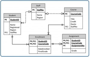
Each enrollment must have a valid student.
Note: Since the StudentID is part of the PK, it can’t be null. Therefore, any StudentID entered, must exist in the Student
table at least once to a maximum of 1 time. This should be obvious since the PK cannot have duplicates.
Figure A.2 by A. Watt.
Refer to Figure A.3. A staff record (a tutor) is associated with a minimum of 0 students to a maximum of many students.
A student record may or may not have a tutor.
Figure A.3 by A. Watt.
Note: The StaffNo field in the Student table allows null values – represented by the 0 on the left side. However, if a
StaffNo exists in the student table it must exist in the Staff table maximum once – represented by the 1.
Refer to Figure A.4. A staff record (instructor) is associated with a minimum of 0 courses to a maximum of many courses.
A course may or may not be associated with an instructor.
Note: The StaffNo in the Course table is the FK, and it can be null. This represents the 0 on the left side of the relation-
ship. If the StaffNo has data, it has to be in the Staff table a maximum of once. That is represented by the 1 on the left
side of the relationship.
Refer to Figure A.5. A course must be offered (in enrollment) at least once to a maximum of many times.
The Enrollment table must contain at least 1 valid course to a maximum of many.
Refer to Figure A.6. An enrollment can have a minimum of 0 assignments or a maximum of many.
An assignment must be associated with at least 1 with a maximum of 1 enrollment.
APPENDIX A UNIVERSITY REGISTRATION DATA MODEL EXAMPLE • 115
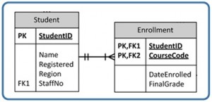
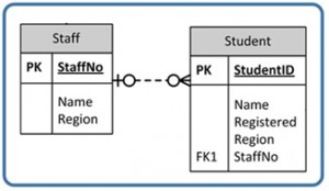
Figure A.4 by A. Watt.
Figure A.5 by A. Watt.
Note: Every record in the Assignment table must contain a valid enrollment record. One enrollment record can be
associated with multiple assignments.
Figure A.6 by A. Watt.
Attribution
This is an adaptation, not a derivation as the author wrote half of it. Source: http://openlearn.open.ac.uk/mod/oucon-
tent/view.php?id=397581§ion=8.2
116 •
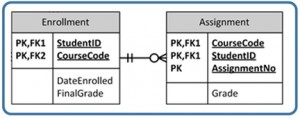
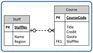
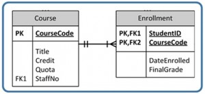
Appendix B Sample ERD Exercises
Exercise 1
Manufacturer
A manufacturing company produces products. The following product information is stored: product name, product ID
and quantity on hand. These products are made up of many components. Each component can be supplied by one or
more suppliers. The following component information is kept: component ID, name, description, suppliers who supply
them, and products in which they are used. Use Figure B.1 for this exercise.
Create an ERD to show how you would track this information.
Show entity names, primary keys, attributes for each entity, relationships between the entities and cardinality.
Assumptions
• A supplier can exist without providing components.
• A component does not have to be associated with a supplier.
• A component does not have to be associated with a product. Not all components are used in products.
• A product cannot exist without components.
ERD Answer
Component(CompID, CompName, Description) PK=CompID
Product(ProdID, ProdName, QtyOnHand) PK=ProdID
Supplier(SuppID, SuppName) PK = SuppID
CompSupp(CompID, SuppID) PK = CompID, SuppID
Build(CompID, ProdID, QtyOfComp) PK= CompID, ProdID
Figure B.1 by A. Watt.
117
Exercise 2
Car Dealership
Create an ERD for a car dealership. The dealership sells both new and used cars, and it operates a service facility (see
Figure B.2). Base your design on the following business rules:
• A salesperson may sell many cars, but each car is sold by only one salesperson.
• A customer may buy many cars, but each car is bought by only one customer.
• A salesperson writes a single invoice for each car he or she sells.
• A customer gets an invoice for each car he or she buys.
• A customer may come in just to have his or her car serviced; that is, a customer need not buy a car to be
classified as a customer.
• When a customer takes one or more cars in for repair or service, one service ticket is written for each car.
• The car dealership maintains a service history for each of the cars serviced. The service records are
referenced by the car’s serial number.
• A car brought in for service can be worked on by many mechanics, and each mechanic may work on many
cars.
• A car that is serviced may or may not need parts (e.g., adjusting a carburetor or cleaning a fuel injector nozzle
does not require providing new parts).
118 •
ERD Answer
APPENDIX B SAMPLE ERD EXERCISES • 119
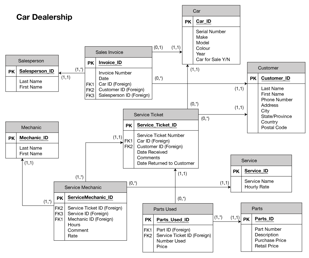
Appendix C SQL Lab with Solution
Download the following script: OrdersAndData.sql.
Part 1 – DDL
Figure C.1. ERD for Orders and Data.
1. Use the script OrdersAndData.sql that creates the tables and adds the data for the Orders and Data ERD in
Figure C.1.
2. Create a database called Orders. Modify the script to integrate the PK and referential integrity. Show the
CREATE TABLE statements with the modifications including the constraints given in step 3.
3. Add the following constraints:
• tblCustomers table: Country – default to Canada
• tblOrderDetails: Quantity – > 0
• tblShippers: CompanyName must be unique.
• tblOrders: ShippedDate must be greater than order date.
120
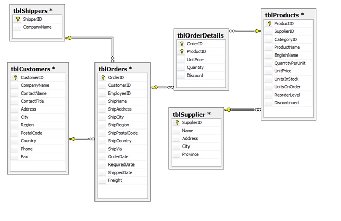
CREATE DATABASE Orders
Go
Use Orders
Go
Use Orders
Go
CREATE TABLE [dbo].[tblCustomers]
[CustomerID] nvarchar(5) NOT NULL,
[CompanyName] nvarchar(40) NOT NULL,
[ContactName] nvarchar(30) NULL,
[ContactTitle] nvarchar(30) NULL,
[Address] nvarchar(60) NULL,
[City] nvarchar(15) NULL,
[Region] nvarchar(15) NULL,
[PostalCode] nvarchar(10) NULL,
[Country] nvarchar(15) NULL
Constraint df_country DEFAULT ‘Canada’,
[Phone] nvarchar(24) NULL,
[Fax] nvarchar(24) NULL,
Primary Key (CustomerID)
);
CREATE TABLE [dbo].[tblSupplier] (
[SupplierID] int NOT NULL,
[Name] nvarchar(50) NULL,
[Address] nvarchar(50) NULL,
[City] nvarchar(50) NULL,
[Province] nvarchar(50) NULL,
Primary Key (SupplierID)
);
Part 2 – Create the Following SQL Statements
1. Show a list of customers and the orders they generated during 2014. Display customer ID, order ID, order date and
date ordered.
2. Using the ALTER TABLE statement, add a new field (Active) in the tblcustomer. Default it to True.
APPENDIX C SQL LAB WITH SOLUTION • 121
CREATE TABLE [dbo].[tblShippers] (
[ShipperID] int NOT NULL,
[CompanyName] nvarchar(40) NOT NULL,
Primary Key (ShipperID),<
CONSTRAINT uc_CompanyName UNIQUE (CompanyName)
);
CREATE TABLE [dbo].[tblProducts] (
[ProductID] int NOT NULL,
[SupplierID] int NULL,
[CategoryID] int NULL,
[ProductName] nvarchar(40) NOT NULL,
[EnglishName] nvarchar(40) NULL,
[QuantityPerUnit] nvarchar(20) NULL,
[UnitPrice] money NULL,
[UnitsInStock] smallint NULL,
[UnitsOnOrder] smallint NULL,
[ReorderLevel] smallint NULL,
[Discontinued] bit NOT NULL,
Primary Key (ProductID),
Foreign Key (SupplierID) References tblSupplier
);
3. Show all orders purchased before September 1, 2012. Display company name, date ordered and total amount of
order (include freight).
SELECT tblOrders.OrderID, OrderDate as ‘Date Ordered’, sum(unitprice*quantity*(1-discount))+ freight as ‘Total
Cost’
FROM tblOrderDetails join tblOrders on tblOrders.orderID = tblOrderDetails.OrderID
WHERE OrderDate < ‘September 1, 2012′
GROUP BY tblOrders.OrderID, freight, OrderDate
4. Show all orders that have been shipped via Federal Shipping. Display OrderID, ShipName, ShipAddress and Cus-
tomerID.
SELECT OrderID, ShipName, ShipAddress, CustomerID
FROM tblOrders join tblShippers on tblOrders.ShipVia = tblShippers.ShipperID
WHERE CompanyName= ‘Federal Shipping’
122 •
CREATE TABLE [dbo].[tblOrders] (
[OrderID] int NOT NULL,
[CustomerID] nvarchar(5) NOT NULL,
[EmployeeID] int NULL,
[ShipName] nvarchar(40) NULL,
[ShipAddress] nvarchar(60) NULL,
[ShipCity] nvarchar(15) NULL,
[ShipRegion] nvarchar(15) NULL,
[ShipPostalCode] nvarchar(10) NULL,
[ShipCountry] nvarchar(15) NULL,
[ShipVia] int NULL,
[OrderDate] smalldatetime NULL,
[RequiredDate] smalldatetime NULL,
[ShippedDate] smalldatetime NULL,
[Freight] money NULL
Primary Key (OrderID),
Foreign Key (CustomerID) References tblCustomers,
Foreign Key (ShipVia) References tblShippers,
Constraint valid_ShipDate CHECK (ShippedDate > OrderDate)
);
CREATE TABLE [dbo].[tblOrderDetails] (
[OrderID] int NOT NULL,
[ProductID] int NOT NULL,
[UnitPrice] money NOT NULL,
[Quantity] smallint NOT NULL,
[Discount] real NOT NULL,
Primary Key (OrderID, ProductID),
Foreign Key (OrderID) References tblOrders,
Foreign Key (ProductID) References tblProducts,
Constraint Valid_Qty Check (Quantity > 0)
);
Go
5. Show all customers who have not made purchases in 2011.
6. Show all products that have never been ordered.
OR
APPENDIX C SQL LAB WITH SOLUTION • 123
Use Orders
Go
SELECT CompanyName, OrderID, RequiredDate as ‘order date’, OrderDate as ‘date ordered’
FROM tblcustomers JOIN tblOrders on tblOrders.CustomerID = tblCustomers.CustomerID
WHERE Year(OrderDate) = 2014
ALTER TABLE tblCustomers
ADD Active bit DEFAULT (‘True’)
SELECT CompanyName
FROM tblCustomers
WHERE CustomerID not in
( SELECT CustomerID
FROM tblOrders
WHERE Year(OrderDate) = 2011
)
SELECT ProductID from tblProducts
Except
SELECT ProductID from tblOrderDetails
SELECT Products.ProductID,Products.ProductName
FROM Products LEFT JOIN [Order Details]
ON Products.ProductID = [Order Details].ProductID
WHERE [Order Details].OrderID IS NULL
7. Show OrderIDs for customers who reside in London. Use a subquery. Display CustomerID, CustomerName and
OrderID.
SELECT Customers.CompanyName,Customers.CustomerID,OrderID
FROM Orders
LEFT JOIN Customers ON Orders.CustomerID = Customers.CustomerID
WHERE Customers.CompanyName IN
(SELECT CompanyName
FROM Customers
WHERE City = ‘London’)
124 •
8. Show products supplied by Supplier A and Supplier B. Display product name and supplier name.
SELECT ProductName, Name
FROM tblProducts JOIN tblSupplier on tblProducts.SupplierID = tblSupplier.SupplierID
WHERE Name Like ‘Supplier A’ or Name Like ‘Supplier B’
9. Show all products that come in boxes. Display product name and QuantityPerUnit.
SELECT EnglishName, ProductName, QuantityPerUnit
FROM tblProducts
WHERE QuantityPerUnit like ‘%box%’
ORDER BY EnglishName
Part 3 – Insert, Update, Delete, Indexes
1. Create an Employee table. The primary key should be EmployeeID (autonumber). Add the following fields: Last-
Name, FirstName, Address, City, Province, Postalcode, Phone, Salary. Show the CREATE TABLE statement and the
INSERT statements for the five employees. Join the employee table to the tblOrders. Show the script for creating the
table, setting constraints and adding employees.
Use Orders
CREATE TABLE [dbo].[tblEmployee](
EmployeeID Int IDENTITY NOT NULL ,
FirstName varchar (20) NOT NULL,
LastName varchar (20) NOT NULL,
Address varchar (50),
City varchar(20), Province varchar (50),
PostalCode char(6),
Phone char (10),
Salary Money NOT NULL,
Primary Key (EmployeeID)
Go
INSERT into tblEmployees
Values (‘Jim’, ‘Smith’, ‘123 Fake’, ‘Terrace’, ‘BC’, ‘V8G5J6′, ‘2506155989’, ‘20.12’),
(‘Jimmy’, ‘Smithy’, ‘124 Fake’, ‘Terrace’, ‘BC’, ‘V8G5J7′, ‘2506155984’, ‘21.12’),
(‘John’, ‘Smore’, ’13 Fake’, ‘Terrace’, ‘BC’, ‘V4G5J6′, ‘2506115989’, ‘19.12’),
(‘Jay’, ‘Sith’, ’12 Fake’, ‘Terrace’, ‘BC’, ‘V8G4J6′, ‘2506155939’, ‘25.12’),
(‘Jig’, ‘Mith’, ’23 Fake’, ‘Terrace’, ‘BC’, ‘V8G5J5′, ‘2506455989’, ‘18.12’);
Go
APPENDIX C SQL LAB WITH SOLUTION • 125
2. Add a field to tblOrders called TotalSales. Show DDL – ALTER TABLE statement.
ALTER TABLE tblOrders
ADD Foreign Key (EmployeeID) references tblEmployees (EmployeeID)
3. Using the UPDATE statement, add the total sale for each order based on the order details table.
UPDATE tblOrders
Set TotalSales = (select sum(unitprice*quantity*(1-discount))
FROM tblOrderDetails
WHERE tblOrderDetails.OrderID= tblOrders.OrderID
GROUP BY OrderID
126 •
About the Authors
Primary Author: Adrienne Watt
Adrienne Watt holds a computer systems diploma (BCIT), a bachelor’s degree in technology (BCIT) and a master’s
degree in business administration (City University).
Since 1989, Adrienne has worked as an educator and gained extensive experience developing and delivering business
and technology curriculum to post-secondary students. During that time, she ran a successful software development
business. In the business, she worked as an IT professional in a variety of senior positions including project manager,
database designer, administrator and business analyst. Recently she has been exploring a wide range of technology-relat-
ed tools and processes to improve delivery methods and enhance learning for her students.
127
Contributing Author: Nelson Eng
Nelson Eng completed his bachelor’s degree in commerce (accounting and management information systems) from the
University of British Columbia and a master’s degree in computer science from the University of Western Ontario.
He spent 11 years as a computer systems coordinator with Science World of B.C. and 14 years as a computer science
and information systems instructor with Douglas College.
128 •
- Database Design - 2nd Edition
- Database Design - 2nd Edition
- Contents
- Preface
- About the Book
- Acknowledgements
- Chapter 1 Before the Advent of Database Systems
- Chapter 2 Fundamental Concepts
- Chapter 3 Characteristics and Benefits of a Database
- Chapter 4 Types of Data Models
- Chapter 5 Data Modelling
- Chapter 6 Classification of Database Management Systems
- Chapter 7 The Relational Data Model
- Chapter 8 The Entity Relationship Data Model
- Chapter 9 Integrity Rules and Constraints
- Chapter 10 ER Modelling
- Chapter 11 Functional Dependencies
- Chapter 12 Normalization
- Chapter 13 Database Development Process
- Chapter 14 Database Users
- Chapter 15 SQL Structured Query Language
- Chapter 16 SQL Data Manipulation Language
- Appendix A University Registration Data Model Example
- Appendix B Sample ERD Exercises
- Appendix C SQL Lab with Solution
- About the Authors