


Week 2 iLab Summit Ridge Mountain Resort
Scenario/Summary
Management at Summit Ridge Mountain Resort is very pleased with your initial report. This week, management has asked that you add to the prior analysis and incorporate some visual images concerning the Village Shop sales. This new analysis will require the use of new formulas, new functions, and several charts to graphically depict the report findings. This updated Excel workbook will be used for a presentation to the board of directors.
Deliverables
Submit one workbook. When submitting the workbook, provide a comment in the comments area explaining what you learned from completing this lab activity.
File naming convention: If your name is Jane Doe, then your file should be named very similar to Doe_J_Week2_Lab.xlsx.
Make certain you compare your finished work with the Grading Rubric included here.
| Lab 2 – Shop Analysis | ||||
| Step | Task | Points Possible | Points Received | Comments |
|---|---|---|---|---|
| Documentation sheet completed | 5 | |||
| 1 | Daily Item Totals worksheet | |||
| 1a | Copy Daily Sales to new worksheet | 2 | ||
| 1b | SUM function for items | 2 | ||
| SUM function for dates | 2 | |||
| 1c | Formula percentage of sales | 3 | ||
| 1d | Statistical functions for sales | 3 | ||
| 1e | Formula profit per item | 2 | ||
| 2 | Create Bar Chart | |||
| 2a | 2D Bar Chart | 5 | ||
| 2b | On new worksheet | 2 | ||
| 2c | Title and tab named | 2 | ||
| 3 | Create Pie Chart | |||
| 3a | Pie Chart | 5 | ||
| 3b | On new worksheet | 2 | ||
| 3c | Title and tab named | 2 | ||
| 4 | Create Weekly Profits | |||
| 4a | Copy Daily Sales to new worksheet | 2 | ||
| 4b | Calculate profit per item | 2 | ||
| 4c | Calculate profits for each item | 4 | ||
| 4d | Autofill profits for all items | 3 | ||
| 4e | Create Line Chart | 5 | ||
| 4f | Title and tab named | 2 | ||
| Comment: What you learned from completing this Lab | 5 | |||
| TOTAL POINTS | 60 | 0 | ||
Week 2 Grading Rubric
Lab Resources
Microsoft Office: Excel 2016
Options for Accessing Microsoft Excel 2016
- Use a personal copy on your PC. You can request a copy of Microsoft Office 2016 via the Student Software Store icon on the Course Resources page.
- If you are a MAC user, click to read the MAC User Information.
- If you do not have Excel 2016 installed locally, then access the software by going to the Course Resources page, Lab Resources section, and click the Virtual Lab Citrix icon.
Lab Steps
Preparation
This lab will use Microsoft Excel 2016.
Be sure you have read the required chapter materials and reviewed the hands-on exercise videos located on the Lesson page before you begin the lab.
Please do not rely solely on the hands-on exercise videos to complete this week’s lab. The videos provide detailed examples, walking you through the hands-on exercises. Applying the hands-on exercise examples will provide both practice and instruction of what to complete.
For example, your final assignment file should include six worksheets (Documentation, Sales Data, Daily Item Totals, Total Items Bar Chart, Percent of Sales Pie Chart, and Profits by Day Line Chart).
Please open the Week 1 Lab submitted and make any corrections or modifications. Save this new Excel workbook as Doe_J_Week2_Lab.xlsx. Follow the lab steps to create formulas, utilize functions, and add charts to graphically depict the sales over time and by product.
Step 1: Create Daily Item Totals Worksheet
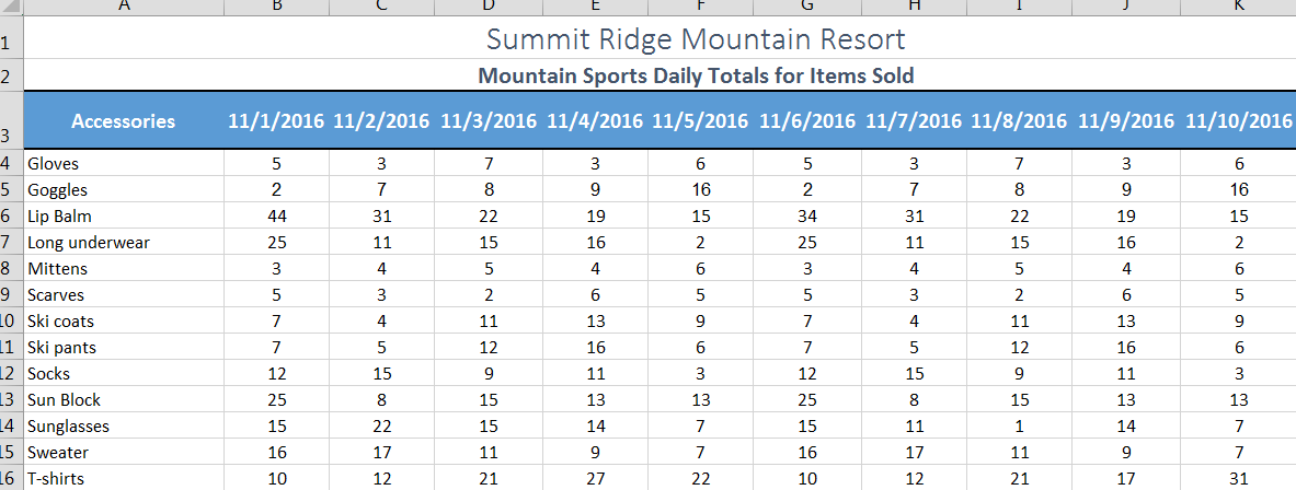
Click on the Sales Data worksheet. We need to see all of the hidden data, so unhide all hidden columns. Once you can see all the hidden data, we need to select data to copy to a new worksheet. Sort your data in A to Z order. Select the accessories data in column A, hold your control key down, and then select the daily sales data in columns D through M. Copy this selected data to a new sheet.

- The Daily Sales data will look as follows on the new worksheet. Please name the tab for this worksheet Daily Item Totals.
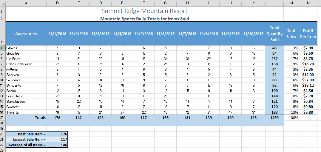
Create daily totals using the SUM function for each day and for each item. Make these pronounced by adding a bold font and some color formatting.

- Let’s add a formula to calculate the percentage of sales for each item in column M. Percent of sales can be determined by dividing the total of each item (L4) by the total of all items (L17).
- Add functions to determine the best sale item, the lowest sale item, and the average of all sale items.
- Last, add a column called Profit per Item. Subtract the cost of the item from net selling price and place it in column N.
Step 2: Create the Total Items Bar Chart
- Using the Daily Item Totals sheet, select the accessories data in column A, hold your control key down, and then select the Total Items Column L. While this data is selected, click the Insert tab on the ribbon. Choose a 2-D Bar Chart.
- Move this chart to a new worksheet.
- Your chart needs a professional title, and the worksheet tab should also be named appropriately.
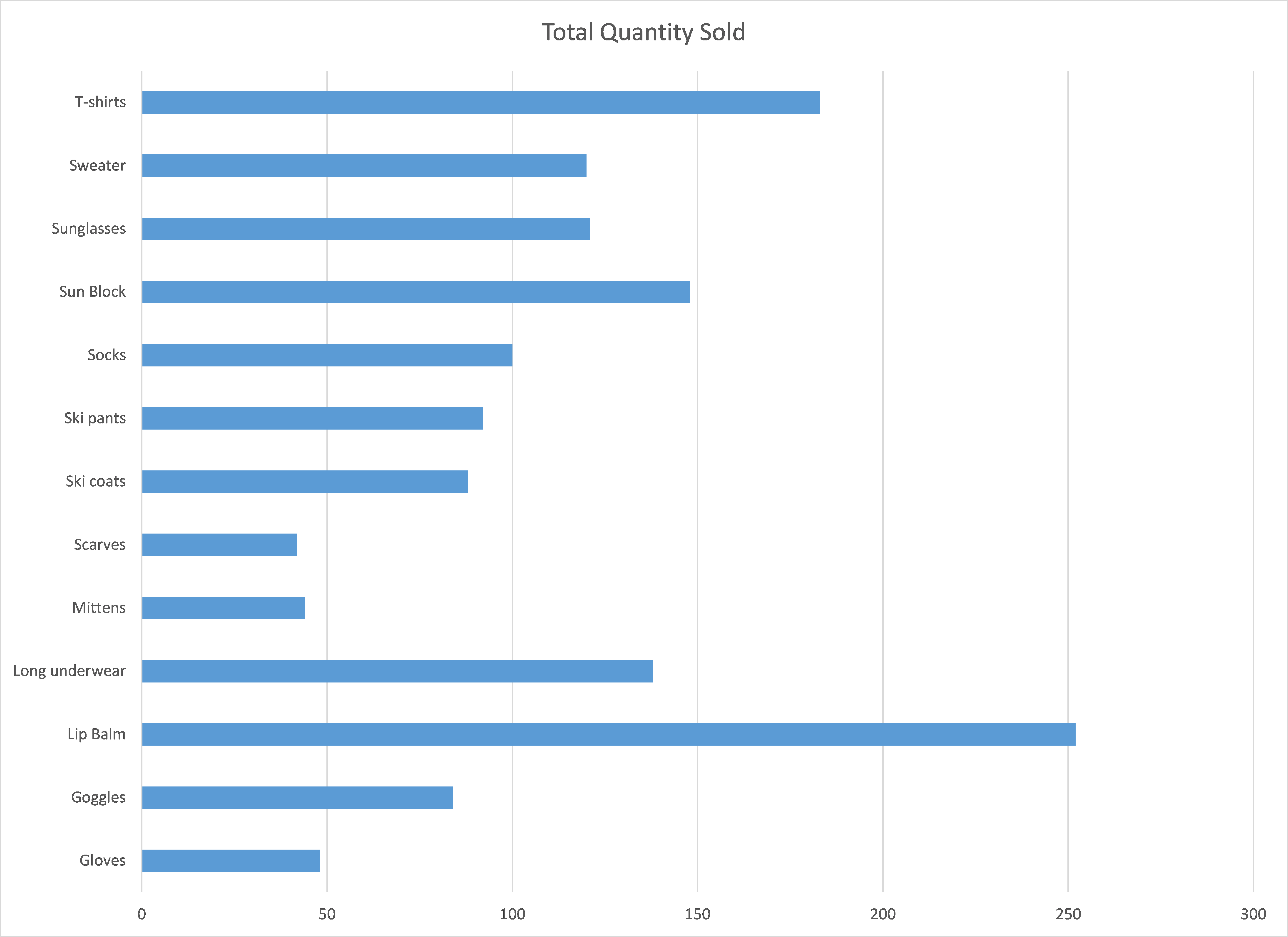 Horizontal Bar Chart
Step 3: Create the Percentage of Sales Pie Chart
- Using the Daily Item Totals sheet, select the accessories data in column A, hold your control key down, and then select the Percent of Sales Column M. While this data is selected, click the Insert tab on the ribbon. Choose a 3-D Pie Chart.
- Move this chart to a new worksheet.
- Your chart needs a professional title, and the worksheet tab should also be named appropriately.
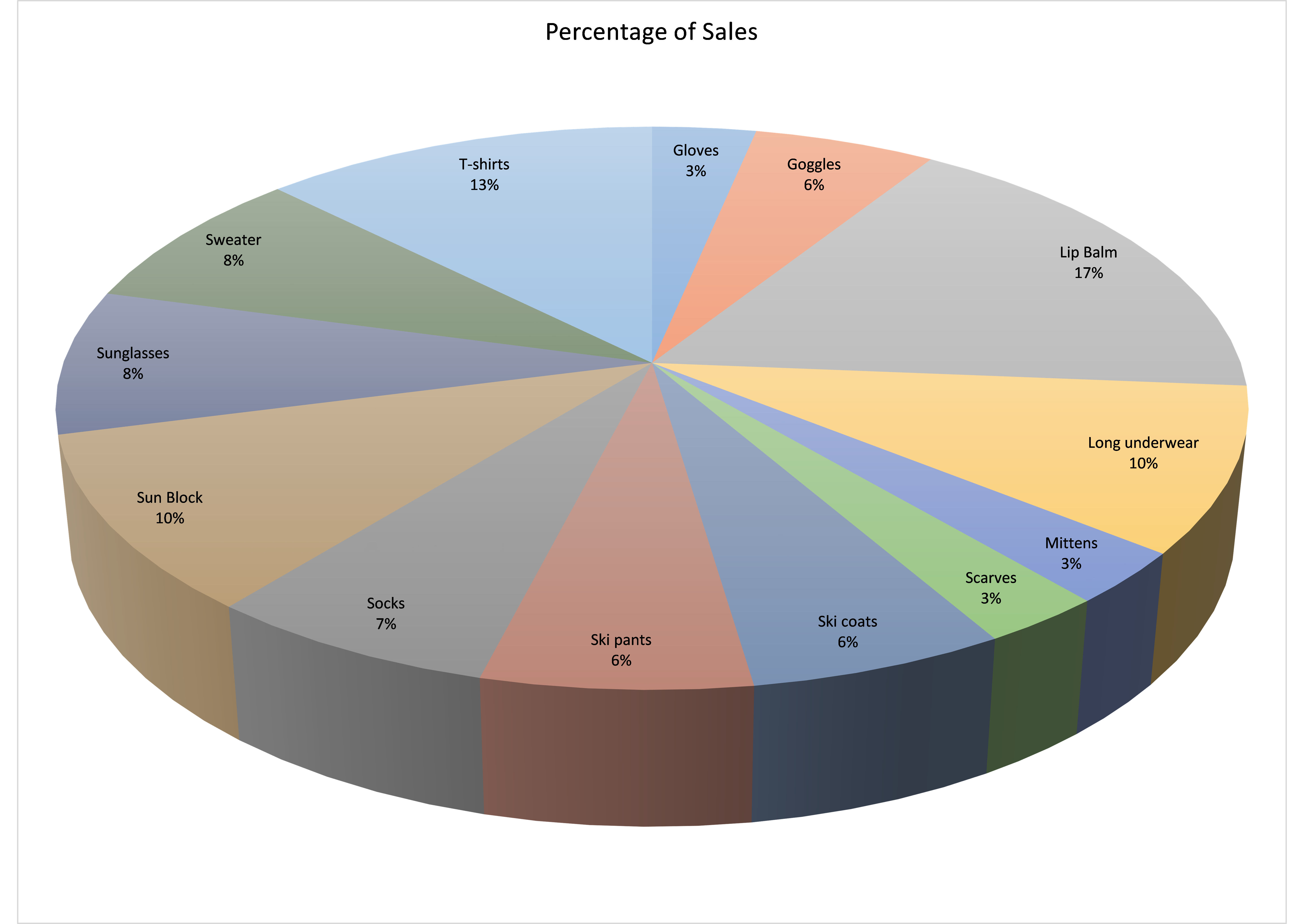 Pie Chart
Step 4: Create Weekly Profits by Item and Line Chart
- Copy the Daily Sales data to a new worksheet.
- Calculate the profit per item. Subtract the cost of the item from the net selling price and place it in column L.
- Next, create a new area on the same worksheet and calculate the profits for each item. For example, the profits for gloves in cell B19 are calculated as B3 * $L3.
- Autofill all weekly profits by item and total.
 Weekly Profits Worksheet
 - Lastly, select the dates across the horizontal, hold down the control key, and select the daily totals along the bottom. Insert a Line Chart like below.
- Give the chart a title, but leave it on the same worksheet.
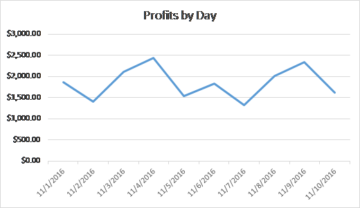 Profits by Day Line Chart
Step 5: Professional Appearance (Cleanup)
Cleanup the formatting of your Excel workbook, taking into account professional appearance.
The Minimum Requirement (per the Grading Rubric)
- Apply a color and assign a descriptive name to each tab (sheet) in the workbook.
- Update the documentation worksheet to include contents of each worksheet.
- Make certain to include a custom page header on the Sales Data worksheet with your name and your instructor’s name.
- Set the page orientation to landscape.
Remember, professional appearance doesn’t only promote better readability of your report but represents you as a professional.
Finish: Save and Submit
Save your Excel file. Saving your file often is good practice (Ctrl + s).
Your Excel file should contain six worksheets.
- Documentation
- Sales Data
- Daily Item Totals
- Total Items Bar Chart
- Percent of Sales Pie Chart
- Profits by Day
Submit one workbook. When submitting the workbook, provide a comment in the comments area explaining what you learned from completing this lab activity.
File naming convention: If your name is Jane Doe, then your file should be named very similar to Doe_J_Week2_Lab.xlsx.
 9 years ago
Purchase the answer to view it

 week2_lab.xlsx

